WHY BOTHER WITH SEX? THE EVOLUTION OF RECOMBINATION IN AN ARTIFICIAL GENE NETWORK MODEL
Alexander O. B. Whitlock
A dissertation submitted to the faculty at the University of North Carolina at Chapel Hill in partial fulfillment of the requirements for the degree of Doctor of Philosophy in the
Curriculum in Genetics and Molecular Biology in the School of Medicine.
Chapel Hill 2016
Approved by: Christina Burch Shawn Gomez Ronald Swanstrom Todd Vision
c 2016
ABSTRACT
Alexander O. B. Whitlock: Why bother with sex? The evolution of recombination in an artificial gene network
(Under the direction of Christina Burch)
TABLE OF CONTENTS
LIST OF TABLES . . . vii
LIST OF FIGURES . . . viii
LIST OF SYMBOLS AND ABBREVIATIONS . . . ix
CHAPTER 1: INTRODUCTION . . . 1
Models of the Evolution of Sex . . . 8
CHAPTER 2: AN EVOLVING GENETIC ARCHITECTURE INTERACTS WITH HILL-ROBERTSON INTERFERENCE TO DETERMINE THE BENEFIT OF SEX . . . 11
Materials and Methods . . . .14
Results . . . 20
Discussion . . . 27
Figures . . . 31
CHAPTER 3: POPULATION SUBDIVISION MAXIMIZES THE SUSTAINABLE COST OF SEX . . . 49
Materials and Methods . . . .46
Results . . . 47
Discussion . . . 50
Figures . . . 53
CHAPTER 4: CONCLUSIONS . . . 60
APPENDIX 1: CHAPTER 2 SUPPLEMENT . . . 69
Reproductive Mode . . . 69
Tables . . . 71
APPENDIX 2: CHAPTER 3 SUPPLEMENT . . . 73
LIST OF FIGURES
1 Sex has a long-term advantage . . . 31
2 Equilibrium mean fitness . . . 32
3 Hill-Robertson interference affected asexual populations of all sizes . . . 33
4 Sex has a short-term advantage in large populations . . . 34
5 Changes in genetic architecture influence the success of sex . . . 35
6 Evolution of recombination rate . . . 36
7 Hill-Robertson interference interacts with evolving genetic architecture . . . 36
8 Evolution of the distribution of mutation effects . . . 37
9 Equilibria and invasion probabilities at low and high mutation rates . . . 38
10 Network connectivity (c) impacts the success of sex. . . 39
11 Relative fixation probabilities (u/u∗) of modifiers of sex. . . 40
12 Relative fixation probabilities (u/u∗) of a modifier of recombination . . . 40
13 Frequency dynamics during successful invasions by modifiers of sex. . . 41
14 Costly sex does not evolve . . . 42
15 Evolution of genetic architecture gives sex an equilibrium advantage . . . 53
16 Operation of Muller’s ratchet maximizes the equilibrium advantage of sex . . 54
17 Sex has an equilibrium advantage . . . 55
18 Equilibrium asexual fitness shows Muller’s ratchet and mutation load . . . . 56
19 Population structure supports maintenance of costly sex . . . 56
20 Wˆsex/Wˆasex converges withCmax in highly structured populations . . . 57
21 Evolving genetic architecture permits the success of costly sex . . . 58
LIST OF SYMBOLS
C Cost of sex
Cmax Maximum cost at which sex is advantageous
FST Wright’s F statistic of population differentiation
LD Linkage disequilibrium
LR Recombination load
m Migration rate
N Population size
Nd Deme size
Ne Effective population size
Tf ix Transit time from mutation to fixation
Ud Deleterious mutation rate
ˆ
V Neutral variance at equilibrium
¯
W Population mean fitness
ˆ
W Population equilibrium mean fitness
ˆ
CHAPTER 1: INTRODUCTION
"We do not even in the least know the final cause of sexuality; why new beings should be produced by the union of the two sexual elements, instead of by a process of parthenogenesis." -Charles Darwin, 1862
Sex is nearly ubiquitous among eukaryotes, with over 99.9% of animals and 99% of plants reproducing sexually at least some of the time (Weismann, 1887; Maynard Smith, 1978; Bell, 1982; Vrijenhoek, 1998; Otto and Lenormand, 2002). Obligate asexual lineages are rare, sparsely speciated, and appear to be short-lived (Bell, 1982), implying bleak odds for long-term success without sex (Judson and Normark, 1996; Little and Hebert, 1996; Birky-Jr., 1996; Normark et al., 2003; Simon et al., 2003). Even bdelloid rotifers, the most notorious exception, share suspiciously similar alleles between otherwise divergent species (Mark Welch et al., 2004; Hillis, 2007), raising the possibility of some form of rare genetic exchange. The prevalence of sexual reproduction would seem to suggest clear benefits and few disadvantages, yet just the opposite is true. A century and a half after Darwin’s observation, the explanation for the origin and maintenance of sex remains one of the most puzzling questions in evolutionary biology.
Sexual reproduction carries the potential for enormous costs (Smith, 1978), including the cost of recombination itself. Because the fitness of a phenotype is the product of selection for combinations of genes that work favorably together, it is not clear how random reshuffling of genes could be advantageous. Given that the immediate effect of recombination is the destruction of beneficial genetic interactions, the resulting fitness decrease should cause recombination to be selected against (Nei, 1967).
population can produce progeny, but sexual population must invest resources in production of two sexes, even if one sex contributes little to the offspring. In organisms which do not produce males, this can instead be thought of as the "two-fold cost of meiosis", or genome dilution, in which each sexual parent contributes only half of its genes to its offspring (Williams, 1975; Lively and Lloyd, 1990). A parent reproducing sexually only propagates 50% of its genome, instead of passing along the entire thing as under clonal reproduction. Therefore, all else (such as fecundity and niche size) being equal, the benefit of sex in organisms paying these
costs must be at least twofold.
Finally, in order to reproduce sexually, individuals must invest time and resources towards finding a mate, which may be especially problematic in a low-density species, making themselves vulnerable to disease and predation in the process.
The population-wide impact of these costs could be alleviated if organisms only engaged in sexual reproduction occasionally and under optimal conditions. Saccharomyces cerevisiae, for example, is facultatively sexual, switching from mitosis to meiosis under low fitness conditions (Hadany and Otto, 2009). However, this facultative sexual reproduction has an additional cost: while mitotic reproduction takes approximately 90 minutes, meiosis lasts on the order of days.
This apparent contradiction, in which a costly strategy is also extraordinarily common, is the paradox of sex. Indeed, the Reduction Principle (Altenberg and Feldman, 1987) states that in a randomly mating population at equilibrium, without mutation, modifiers of recombination can only decrease in a population. One of the first explanations proposed is that sex produces the genetic variation required for adaptation (Weismann, 1887). Though this concept is intuitively appealing, it is not a sufficient explanation because sex does not necessarily increase variation, and when it does, this variation may be maladaptive.
from Hardy-Weinberg proportions. Asexual reproduction will maintain the distribution built by selection, but sexual reproduction restores Hardy-Weinberg proportions, producing intermediate genotypes at the expense of extreme genotypes.
Second, sex may generate genetic variation that is maladaptive. For example, the sickle cell trait is strongly advantageous when heterozygous. Were reproduction to occur asexually, heterozygotes would be expected to go to fixation in the population, resulting in a population free of both sickle cell anemia and malaria. However, sexual reproduction restores the genotypes to Hardy-Weinberg proportions. Though this does increase variance, it does so at a cost to mean fitness. While these examples are obviously not universally applicable, they do demonstrate a need for a more sophisticated explanation.
As may be expected for such a long-lived problem, over 20 hypotheses have been proposed to explain the prevalence of sex. While explanations predicting a direct physiological benefit to sex have been proposed, the most accepted hypotheses predict the benefit is indirect, in which the benefit of sex is its ability to break up linkage disequilibrium (LD). When LD is predominantly negative, that is, when genotypes of intermediate fitness are overrepresented in the population relative to expectations based on allele frequency, natural selection is less efficient. Recombination regenerates extreme phenotypes, restoring the additive genetic variation required for efficient selection (Feldman et al., 1980). Expectations regarding the source of LD and the specific benefit of destroying it can be placed in three categories: The Mutational Deterministic Hypothesis, Red Queen, and Hill-Robertson interference, each of which will be be discussed further.
genome dies or fails to reproduce, those mutations will be purged from circulation (Kimura and Maruyama, 1966; Kondrashov, 1982, 1984). Because sexual reproduction facilitates the removal of deleterious alleles, sexual populations have a lower mutation load than asexual populations.
This prediction requires two things: first, a high genomic mutation rate. A genomic mutation rate of U >= 1 is predicted to have a high enough deleterious mutation supply for the benefits to surpass the twofold cost (Kondrashov, 1993). Second, epistasis must be weak and negative in order to create persistent negative associations between loci (Barton, 1995). However, the conditions that support MDH’s role in selection for recombination may not be widespread in nature. Genomic mutation rates have been quantified for a variety of organisms and, while some do seem to be above 1, including Drosophila (Haag-Liautard et al., 2007) and C. elegans (Denver et al., 2004), many are much lower (Drake et al., 1998). Additionally, empirical evidence for the sign of epistasis is mixed and evidence exists for negative positive, and no epistasis. Indeed, studies find variation in how genes interact, both between organisms and within genomes (Rice, 2002; Kouyos et al., 2007; Whitlock et al., 1995; Elena and Lenski, 1997; de Visser and Elena, 2007). Neither is there evidence that synergistic epistasis evolves as a result of recombination (Desai et al., 2007; MacCarthy and Bergman, 2007). As the parameter requirements seem to be rarely met, MDH is not likely a major contributor to the success of sex.
strong selection, frequent optimum shifts, and high recombination rates, a model implemented by (Hamilton, 1980) demonstrated that sex was able to overcome a two-fold cost.
The negative frequency-dependent selection that results from antagonistic coevolution between species, most notably between hosts and parasites, can produce optimum shifts of this nature (Jaenike, 1978; Hamilton, 1980). Antagonistic coevolution causes fluctuation in linkage disequilibrium and epistasis in both parasites and their hosts (Peters and Lively, 1999) leading to a predicament similar to Lewis Carroll’s Red Queen, in which both species must evolve as quickly as they can just to stay in the same place relative to one another (Bell, 1982).
Both experimental and empirical evidence support a role for parasitic interactions in the frequency of sex. Frequency of sexual reproduction in P. antipodarum correlates with the density of trematode parasites, with asexual reproduction predominating in regions with low parasite load (Lively, 1987; Jokela et al., 2009), with additional evidence of negative frequency-dependent selection, in which the asexual clones which reached high frequency were driven to low frequency or extinction, while sexual reproduction resulted in population stability (Jokela et al., 2009). Experimental coevolution between hosts and parasites has demonstrated time-lagged, frequency-dependent selection (Britt Koskella, 2007), and hosts in populations with high rates of pathogen or parasite infection evolved increased recombination rates (Morran et al., 2009, 2011) both of which support a role for antagonistic coevolution in the maintenance of sex. Generally, there is a pattern of increased prevalence of sexual reproduction in regions with high density of parasites (Neiman et al., 2009), and it has been proposed that the strong positive correlation between longevity, small brood size, and recombination rate demonstrates that recombination is favored in long-lived organisms as a way to create offspring that are relatively resistant to rapidly evolving parasites (Burt and Bell, 1987).
(May and Anderson, 1983; Howard and Lively, 1994; Otto and Nuismer, 2004) and linkage disequilibrium must cycle rapidly, on the order of every two to five generations (Barton, 1995). This is especially problematic because in many organisms, the part of the genome under selection for host-parasite interaction is confined to a single region, yet the entire genome pays the cost of recombination. Simulations with diploid populations are even less likely to find a benefit to sex (Agrawal and Otto, 2006). As a result, the extent to which antagonistic coevolution contributes to the broad maintenance of sex is not clear.
Sex can also act to destroy selection interference among loci. Though the previous hypotheses have been purely deterministic, real populations are finite, and genetic drift also influences the evolution of the population. In a finite population without recombination, linkage disequilibrium accumulates due to a combination of mutation, selection, and drift. This results in Hill-Robertson interference, in which selection at one locus interferes with selection at another linked locus (Hill and Robertson, 1966; Felsenstein, 1974; Comeron et al., 2008). By destroying linkage disequilibrium, sex exposes the loci to selection. Hill-Robertson interference can take at least four forms.
2005).
In a linked genome, the fate of a new mutation is inextricably tied to the genetic background in which it arises, regardless of its individual selection coefficient. In a linked genome containing both a beneficial and a deleterious mutations, the apparent fitness consequence of each is decreased by its counterpart, forestalling efficient selection for or against either mutation. As a result, a beneficial mutation that arises in an otherwise low-fitness linked genome may be lost due to background selection (Charlesworth, 1993b; Peck, 1994; Charlesworth, 1994). Similarly, a deleterious mutation in an otherwise high fitness linked genotype may hitchhike to fixation (Maynard Smith and Haigh, 1974; Peck, 1994; Bachtrog and Gordo, 2004; McDonald et al., 2016). Both hitchhiking and background selection decrease the effective population size. By freeing mutations from the genetic background in which they arose, recombination increases additive genetic variance and allows efficient selection.
Muller’s ratchet is predicted to have the strongest effect in small populations, where genetic drift has the most influence. Over time, genetic drift stochastically causes fixation of deleterious mutations. With each fixation event, the number of accumulated mutations in the least-loaded genotype increases by one, and barring a rare beneficial mutation or back-mutation, the population’s fitness has been irrevocably decreased (Muller, 1964; Felsenstein, 1974; Haigh, 1978; Gordo and Charlesworth, 2000). To use Muller’s analogy, the ratchet has been tightened a click. As mutations accumulate, the ratchet continues to tighten, with the potential for a mutational meltdown and the loss of the asexual population (Haigh, 1978; Lynch and Gabriel, 1990; Gabriel et al., 1993). Sexual recombination, however, can halt the ratchet. Recombination between two unfit genotypes can restore the most fit ancestral genotype and salvage the population. Though evolution of compensatory interactions can avert Muller’s Ratchet in some instances (Poon and Otto, 2000; Silander et al., 2007; Neher and Shraiman, 2012), other populations have been observed to undergo mutational meltdowns and extinction (Higgins and Lynch, 2001).
all populations are finite and subject to some level of drift, is expected to function broadly (Comeron et al., 2008). It is less dependent on epistasis than other models, and has been demonstrated to support the evolution of sex given positive, negative or absent epistasis (Felsenstein and Yokoyama, 1976; Otto and Barton, 2001; Barton and Otto, 2005). Even though it is drift-based, it does not require an especially small population size. In a large population size, increasing the number of loci under selection increases the potential for linkage to affect genetic variation (Iles et al., 2003). The addition of structure to large populations introduces the potential for substantial genetic drift within demes (Martin et al., 2006). As a result, Hill-Robertson interference is of particular interest as an explanation for the prevalence of sexual reproduction due to its apparent ability to promote a strong advantage of sex across a wide parameter range (Otto and Barton, 2001; Iles et al., 2003; Barton and Otto, 2005; Keightley and Otto, 2006; Gordo and Campos, 2008; Hartfield et al., 2010, 2012).
MODELS OF THE EVOLUTION OF SEX
"So far, we have been able to study only one evolving system and we cannot wait for interstellar flight to provide us with a second. If we want to discover generalizations about evolving systems, we will have to look at artificial ones." -John Maynard Smith, 1992
Computational models both complement and extend results from biological organisms. Not only are results from simulations more repeatable and analyzable, thousands of generations of evolution can be simulated in a afternoon. The compromise is that such scale necessitates simplifications. As it is said, "All models are wrong, but some are useful" (Box, 1979). A model falls into the latter category only to the extent that its simplifications do not affect its results.
2008)–do not evolve. While this assumption may be appropriate if genetic architecture did not interact with sex, there is substantial evidence that it is otherwise. For example, many models are based on a simplified two or three locus model (McVean and Charlesworth, 2000; Gardner and Kalinka, 2006; Livnat et al., 2008, 2010; Hodgson and Otto, 2012; Park and Krug, 2013), even though real genomes are larger and more complex, a property which has been shown to increase the benefit of sex (Lenski et al., 1999; Iles et al., 2003; Sanjuán and Elena, 2006; Charlesworth et al., 2009; Barbuti et al., 2012). Other models have used only deleterious mutations (Keightley and Otto, 2006; Gordo and Campos, 2008), or assumed that the distribution of mutational effects is constant (McVean and Charlesworth, 2000; Wilke, 2004; Charlesworth et al., 2009; Barbuti et al., 2012; Park and Krug, 2013). Yet, mutations can be deleterious, neutral or beneficial (Sanjuán et al., 2004), and the distribution of mutational effects can evolve in just a few generations (Burch and Chao, 2004; Montville et al., 2005; Sanjuán et al., 2007; Silander et al., 2007).
Most significantly, recombination itself influences the evolved properties of genetic architec-ture (Azevedo et al., 2006; Gardner and Kalinka, 2006; Misevic et al., 2006; MacCarthy and Bergman, 2007; Livnat et al., 2008; Martin and Wagner, 2009; Livnat et al., 2010; Lohaus et al., 2010), and the genetic architecture that evolves under sexual reproduction has the potential to shape the benefits of sex (Kondrashov, 1982, 1988; Charlesworth, 1990; Otto and Feldman, 1997). As a consequence, omitting evolution of genetic interactions has the potential to change both the mechanism and the impact of sex.
CHAPTER 2: AN EVOLVING GENETIC ARCHITECTURE INTERACTS WITH HILL-ROBERTSON INTERFERENCE TO DETERMINE THE BENEFIT OF SEX
The vast majority of organisms alive today have experienced some form of genetic exchange, or sex, in their recent evolutionary history, despite substantial costs (Weismann, 1887; Maynard Smith, 1978; Bell, 1982; Otto and Lenormand, 2002). Sex breaks up favorable genetic combinations and increases the risk of transmission of pathogens and selfish genetic elements. Sexual reproduction is often slower than asexual reproduction. In many sexually reproducing eukaryotes, sex involves costs of finding and attracting a mate, and of mating in itself; in anisogamous species, if one sex contributes little to progeny production, sexual reproduction carries a two-fold cost of producing that sex. The ubiquity of sex implies that it must confer considerable benefits to overcome these costs. However, the nature of these benefits is not well understood. In fact, over twenty hypotheses have been proposed to explain the benefits of sex (Bell, 1982; Kondrashov, 1993; Hurst and Peck, 1996; Otto and Lenormand, 2002). While hypotheses predicting direct benefits exist (e.g., improved DNA repair, Bernstein et al., 1985), the main benefits of sex are believed to be indirect, such as increased evolvability (Weismann, 1887; Maynard Smith, 1978; Bell, 1982; Kondrashov, 1993; Burt, 2000; Otto and Lenormand, 2002).
Indirect benefits of sex result from the ability of recombination to break down the linkage disequilibrium (LD) generated by mutation, genetic drift, and natural selection. If LD is predominantly negative, that is, if genotypes with the highest and lowest fitness are
1This chapter previously published as an article in Genetics. The original citation is as follows: Whitlock, A.
O. B., Peck, K. M., Azevedo, R. B. R. and Burch, C. L. (2016) "An Evolving Genetic Architecture Interacts
underrepresented in the population, then recombination can generate these extreme genotypes and increase the efficiency of natural selection (Otto and Lenormand, 2002). In the absence of recombination, negative LD can accumulate in a population either through the action of natural selection alone (Red Queen hypothesis: Hamilton 1980; Mutational Deterministic hypothesis: Kimura and Maruyama 1966; Kondrashov 1982, 1988; Charlesworth 1990; Barton 1995; Otto and Feldman 1997), or through the combined actions of selection and genetic drift (Hill-Robertson interference: Hill and Robertson 1966; Felsenstein 1974; Comeron et al. 2008). Although there is evidence supporting the existence of Red Queen and Mutational Deterministic benefits of sex in specific populations, the conditions required to generate these benefits are thought to be too restrictive to provide a general explanation for the ubiquity of sex (Charlesworth, 1993a; Barton, 1995; Otto and Feldman, 1997; Otto and Nuismer, 2004). In contrast, Hill-Robertson interference is thought to operate broadly (Comeron et al., 2008), and to provide strong benefits of sex (Otto and Barton, 2001; Iles et al., 2003; Barton and Otto, 2005; Keightley and Otto, 2006; Gordo and Campos, 2008; Hartfield et al., 2010).
The relative strength of the benefits of sex arising from these different forms of Hill-Robertson interference are known to depend critically on population size and on the distri-bution of mutational effects on fitness. For example, Muller’s ratchet is strongest in small populations that often experience deleterious mutations, whereas the Fisher-Muller effect is strongest in large populations that often experience beneficial mutations. The increase in the strength of the Fisher-Muller effect between beneficial mutations with population size is intuitive because population size (N) affects the beneficial mutation supply rate (N Ub, where
Ub is the beneficial mutation rate). More surprising is the recent finding from evolutionary simulations that interference between deleterious mutations can, on its own, also generate a large benefit of sex that increases with population size (Otto and Barton, 2001; Iles et al., 2003; Barton and Otto, 2005; Keightley and Otto, 2006; Gordo and Campos, 2008; Hartfield et al., 2010). This finding is surprising because neither Muller’s Ratchet (Muller, 1964; Haigh, 1978; Gordo and Charlesworth, 2000) nor background selection (Hudson and Kaplan, 1994, 1995) is expected to increase in strength with population size. The mechanism underlying the dependency of the benefit of sex on population size was little explored in this previous body of work and will be our focus here.
1997). These properties can evolve in just a few generations (Burch and Chao, 2004; Montville et al., 2005; Sanjuán et al., 2007; Silander et al., 2007). We know, from both theoretical (Poon and Otto, 2000) and empirical (Silander et al., 2007) studies, that an evolving genetic architecture impacts the benefits of sex in populations that are sufficiently small to be subject to Muller’s ratchet. As the fitness of asexual populations declines through operation of the ratchet, the rate of compensatory mutations increases, eventually halting the ratchet and limiting this cost of asexuality. We know less about how an evolving genetic architecture impacts the benefit of sex in large populations.
In previous work, we studied a gene network model that explicitly incorporates an evolving genetic architecture (Wagner, 1996; Siegal and Bergman, 2002) and found that sex selects for a lower deleterious mutation rate, lower recombination load, and negative epistasis (Azevedo et al., 2006; Lohaus et al., 2010), three changes in the genetic architecture predicted to favor the maintenance of sex. We noticed that population size affected the extent to which sexual reproduction led to an increase in mean fitness at equilibrium (the long-term advantage) and successfully invaded asexual populations (the short-term advantage), but we did not systematically explore these effects (Lohaus et al., 2010).
advantages of sex increased.
MATERIALS AND METHODS
Our gene network model is based on a model introduced by Wagner (1994, 1996). A haploid genotype is modeled as a network of n genes, each encoding a transcription factor that can, potentially, regulate its own expression or the expression of other genes. The gene network is represented by an n×n matrix,R, where rij ∈R is the regulatory effect of the product of gene j on gene i. Thus, rowi of Rrepresents gene i, including its cis-regulatory elements. Genes are evenly distributed on a linear chromosome in the same order as the rows in the R matrix (i = 1,2, . . . , n). Genes 1 and n are at a map distance λ from each other. Adjacent pairs of genes are at a map distance λ/(n−1) from each other.
The expression pattern of an individual, the Phenotype, is represented by the vector S, where si ∈S is the expression state of gene i= 1,2, . . . , n. Expression states are discrete: a gene is either on (si = +1) or off (si =−1).
The expression pattern of an individual at time t is given by the system of difference equations:
si(t+ 1) =f
" n X
j=1
rijsj(t)
#
(1)
where f is a step function that determines how the input from the gene network controls the expression of the target gene:
f(x) =
+1 if x≥0
−1 if x <0
Starting from an initial gene expression patternS(0)at timet= 0, gene expression changes according to Equation 1 and is judged to reach a steady state if the following criterion is met: S(t) =S(t−1). If a genotype does not achieve a gene expression steady state within
Most random genotypes (see below) fail to produce a gene expression steady state (Pinho et al., 2014).
The fitness of a viable genotype is given by:
W = exp
"
−D(ˆS,S˙)
σ
#
(2)
where D(S,S0) = Pn
i=1(si−s
0
i)2/(4n) measures the difference between expression patterns S and S0,Sˆ is the phenotype corresponding to the genotype, S˙ is the optimal phenotype, and
σ >0 is inversely related to the strength of stabilizing selection.
A random genotype is created by generating a random gene network, R, and a random initial gene expression pattern, S(0). A random gene network is generated by randomly assigning to its rij regulatory elements (1−c)n2 zeros and cn2 non-zero random variates drawn from a standard normal distribution (i.e., with zero mean and unit variance), wherec
is the connectivity density of the network. Networks with more than one weakly connected component (Newman, 2010) are discarded. A random initial gene expression pattern is generated by filling then entries of S(0) with either −1 or+1 with equal probability.
Evolution is simulated using an individual-based, Wright-Fisher model with constant popu-lation size,N, and non-overlapping generations. Individuals undergo a selection-reproduction-mutation life cycle. At the beginning of a simulation, a viable random genotype is cloned
N times to found a population. The optimal phenotype is defined as the phenotype of the founder. This aspect of the environment remains constant throughout the simulation.
matrix of the other parent is copied instead. The process repeats for each row, switching between parents each time a crossover location is encountered. For each offspring, the number of crossovers is drawn randomly from a Poisson distribution with mean 2λ, where λ is the genetic map length in M (morgans). Crossover locations are chosen randomly and occur between genes. No crossovers occur within the regulatory regions of a gene, maintaining each row as a completely linked locus. Unless otherwise stated, sexual reproduction occurs with free recombination (i.eλ/(n−1) = 0.5M).
Both asexually and sexually produced offspring inherit the initial pattern of gene expression,
S(0), of the parents. This aspect of the environment also remains constant throughout the simulation.
Each individual offspring acquires a random number of mutations drawn from a Poisson distribution with mean U, the genomic mutation rate. A mutation is represented by a change to the value of one of the dn2 nonzero regulatory elementsrij, chosen at random; the mutated value is drawn randomly from a standard normal distribution. Mutation cannot create new regulatory interactions (i.e., a zero entry cannot become nonzero), but can transiently remove regulatory interactions (i.e., a nonzero entry may become approximately zero).
The reproductive mode of an individual is determined by its genotype at a modifier locus M. Unless otherwise stated, the M locus is unlinked to the genes involved in the gene network. There are two alleles at the modifier locus: m and M. We have implemented three different genetic bases for these reproductive modes, described below. Under all implementations, if a population is fixed for the m allele every individual reproduces asexually, and if it is fixed for the M allele every individual reproduces sexually. Thus, we refer to the m and M alleles as beingfor asexual and sexual reproduction, respectively. In all simulations where the M locus modifies reproductive mode, the m allele specifies no recombination (i.e.,λ= 0 M), and the
M allele specifies free recombination (i.e., λ/(n−1) = 0.5 M).
One individual is chosen for every reproductive event with probability proportional to its fitness. If it carries the m allele, it reproduces asexually. If it carries the M allele, a second individual carrying an M allele is chosen with probability proportional to its fitness, and the two individuals reproduce sexually and produce one recombinant offspring.
In the Recessive Sex method of reproduction, asexual individuals always reproduce asexually; sexual individuals sometimes reproduce asexually. Two individuals are chosen for every reproductive event with probability proportional to their fitness. If one or both of the individuals carries the m allele, one of them reproduces asexually, regardless of its genotype at the M locus. If both individuals carry the M allele, they reproduce sexually and produce one recombinant offspring.
In the Dominant Sex method of reproduction, sexual individuals always reproduce sexually, but they may recombine with asexual individuals. Two individuals are chosen for every reproductive event with probability proportional to their fitness. If both individuals carry the m allele, one of them reproduces asexually. If one or both of the individuals carry theM
allele, they reproduce sexually and produce one recombinant offspring. The offspring inherits one of the parental alleles at the M locus, chosen randomly.
Fitness variation is given as the mean fitness (W) and mean log fitness (lnW) of all individuals present in the population at a given time (see Equation 2). Genetic variance in log fitness is the total variance in lnW among all individuals present in the population at a given time.
Mean and variance in log fitness under linkage equilibrium is calculated as mean and variance in lnW for a population with the same allele frequencies but no LD (Barton, 1995). We estimated these parameters from a sample of 100 “chimeras.” A chimeric R matrix was constructed by picking each row from the R matrices of any individual in the population with equal probability.
neutral locus acquired a random number of mutations drawn from a Poisson distribution with mean 1. Each mutation added to the neutral locus value a random draw from the standard normal distribution. The equilibrium variance( ˆV)at an unlinked neutral locus is expected to be N, the census population size. We calculatedNe asVˆ at the neutral locus. Ne estimates were obtained at generation 104, at which time all but the largest populations (N = 104) had
achieved equilibrium variance at the neutral locus.
The deleterious mutation rate is defined as Ud = U(pd+pl), where U is the genomic mutation rate, andpdandpl are the proportion of non-lethal deleterious and lethal mutations, respectively (see Box 1). U is constant throughout the course of a simulation but pd and pl can evolve. We estimate the quantity pd+pl for a genotype by generating 100 copies of the genotype carrying a single mutation and evaluating the proportion of them that have lower fitness than the original genotype.
Recombination load is defined as LR =ω−ρ, where ω is the mean fitness of a pair of parental genotypes and andρis the fitness of a single recombinant offspring from them, without mutation (see Box 1). LR was calculated by averaging this measure across N independently chosen pairs of individuals, where each parent was chosen with probability proportional to their fitness (i.e., in the same way the population reproduced in the evolutionary simulations).
We define multiplicative epistasis between two mutations, i and j, as ε = Wi,j/W −
WiWj/W2, where W is the fitness of the unmutated (test) genotype, Wi and Wj are the fitnesses of the single mutants, and Wi,j is the fitness of the double mutant. Otto and Feldman (1997) introduced the standardized epistasis coefficient ε∗ = ε/s¯2, where s¯ = (Wi+Wj)/(2W)−1is the mean effect of a single mutation. We calculated means and variances of ε∗ across pairs of random non-lethal deleterious mutations, introduced individually and in combination into a random sample of 100 viable individuals without replacement (for
N <100, we sampled 100 viable individuals with replacement).
For invasion analysis, populations were evolved for 104 generations under either asexual or
to allow sufficient time for the population to approach mutation-recombination-selection-drift equilibrium. We then mutated the allele at the modifier locus M (see Reproductive mode, above) in a single randomly chosen individual. In most population size× reproductive mode treatments, we measured the fixation probability of the novel modifier allele, u, relative to that of a neutral mutation (u∗ = 1/N) inN replicate invasion trials per independently evolved population, for a total of 50N replicates. For the largestN = 104 populations, computational time limited us to 5N replicate asexual invasion trials and 10N replicate sexual invasion trials.
To measure evolution of recombination rate, populations were evolved for 104 generations
with a modifier locus that was linked to a randomly chosen row of the R matrix and fixed for an allele that specified a map length ofλ = 0M. After generation 104, the modifier locus
experienced mutations at a rate of10−3 per generation. Mutational effects on λ were ±0.05
M, with equal probability. Alleles conferring λ <0 were discarded. When two individuals with map lengths λ1 and λ2 reproduced, the expected number of crossovers in the offspring
was λ1+λ2.
The parameter values used here differed from those used in previous work on the evolution of genetic architecture (Siegal and Bergman, 2002; Azevedo et al., 2006; MacCarthy and Bergman, 2007; Lohaus et al., 2010): the random gene networks were larger (n = 100
genes) and sparser (c= 0.05), and the genomic mutation rate was higher (U = 1). These modifications have three advantages. First, the greater number of genes allows mutations to have a broad range of potential fitness effects, including beneficial, neutral, slightly deleterious and lethal. Second, the higher U allows populations to show considerable mutation load at equilibrium (Martin and Wagner, 2009). Third, real gene networks are relatively sparse (Leclerc, 2008).
All statistics were conducted using the R statistical package, version 3.2.1 (Ihaka and Gentleman, 1996). Comparisons of evolutionary trajectories were conducted using the function
In these models, ln(Time) in generations, Sex (i.e., reproductive mode: sexual or asexual), and ln(N)were modeled as fixed effects. Statistical tests using linear models with only one fixed effect or with multiple fixed effects are described inline or in a detailed table, respectively. In all linear models, population founder was modeled as a random effect.
RESULTS
Sex has a long-term advantage. We simulated the evolution of haploid gene networks in populations ranging in size fromN = 10to104 individuals. We set the genomic mutation rate
to be high(U = 1)and stabilizing selection to be moderate (σ= 0.2) to ensure the operation of all components of Hill-Robertson interference: Muller’s ratchet in smaller populations, the Fisher-Muller effect in larger populations, and hitchhiking and background selection at all population sizes. Mutants differing from the target expression state at i and i+ 1
genes differed in fitness by no more than 5% (i.e., Wi−Wi+1 <0.05, for all i). Populations
were evolved for 104 generations, allowing sufficient time for populations of all sizes to
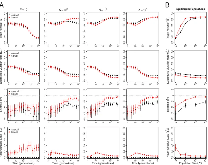
approach mutation-recombination-selection-drift equilibrium. To examine the evolutionary contributions of changes in the genetic architecture in these populations, we monitored mean fitness (W), deleterious mutation rate(Ud), epistasis(ε∗), and recombination load (LR) over the course of the simulations (Figure 1, note that time is plotted on a log scale).
Over the short term (generations 1 through 10), the most striking difference between sexual and asexual populations is that mean fitness declines significantly more quickly in large sexual populations than in large asexual populations (statistical analysis in Appendix table 1). This pattern characterizes populations of at least 100 individuals (ln(Time) × Sex interaction estimated separately for each N ≥100: |t| ≥ 3.989, d.f.= 447, p <0.0001, all tests) and appears to be largely the result of the recombination load increasing in sexual populations through generation 10 (effect of ln(Time) on LR: |t| = 3.975, d.f. = 1699,
p <0.0001). Smaller populations did not show a significant change in mean fitness in the first
Over the longer term (at 104 generations; Figure 1B), sexual populations evolved
signifi-cantly higher mean fitness at equilibrium than asexual populations (cWsex >cWasex), and the
magnitude of the difference depended on population size (Appendix table 2). In populations of 100 individuals or fewer, the difference appears primarily attributable to Muller’s ratchet, as all asexual populations in this size range exhibited a fitness decline between generations 100 and 104 (Figure 1A; effect of ln(Time) on mean fitness estimated separately for each
N ≤100: |t| ≥8.469,d.f.= 399,p < 0.0001, all tests). Only the smallest sexual and asexual populations (N = 10) evolved to indistinguishable equilibrium mean fitnesses, suggesting that the costs of recombination load in sexual populations and of Muller’s ratchet in asexual populations were of similar magnitude at this population size.
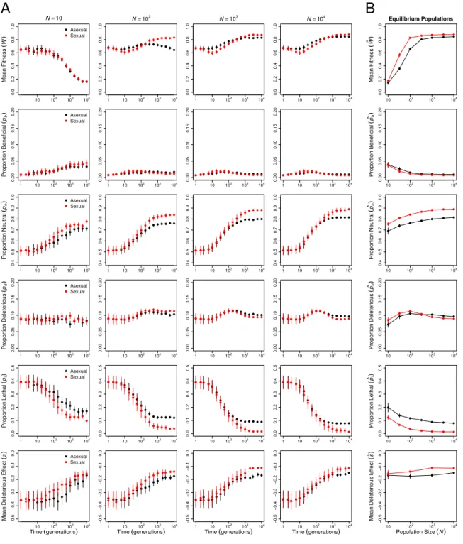
In populations of more than 100 individuals, the equilibrium mean fitness was determined by the evolving genetic architecture (Figure 1B). Both the deleterious mutation rate, Ud (Appendix table 3; p < 0.0001), and the recombination load, LR (in sexuals: |t| = 7.251,
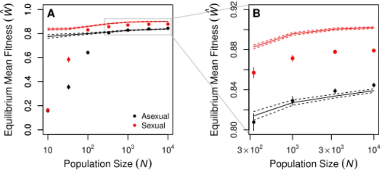
d.f.= 299, p <0.0001), decreased significantly with population size. The proportions of all types of mutations—beneficial, neutral, deleterious, and lethal—evolved, but reductions in the proportion of lethal mutations (pl) and parallel increases in the proportion of neutral mutations (pn) made the strongest contributions to the decreases in Ud (Figure 8). The equilibrium mean fitness of large populations was well predicted by the mutation-selection balance equation (Wc≈e−Ud; Figure 2), with large asexual populations closely matching the
prediction (all N ≥333 differing by <1%) and sexual populations falling slightly below the prediction due to recombination load (all N ≥100 differing by >2.5%).
higher fitness at equilibrium than that predicted by the mutation-selection balance equation. We found the opposite pattern (Figure 2).
Although the operation of Muller’s ratchet (Kimura et al., 1963) was apparent only in populations of 100 individuals or fewer (cW e−Ud; Figure 2), Hill-Robertson interference
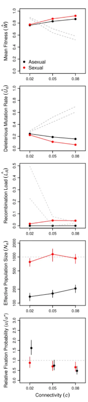
was also operating in larger asexual populations. Background selection reduced neutral genetic variation, a metric ofNe, significantly more in large asexual populations than in small asexual populations (Figure 3B and Appendix table 4). Thus, Hill-Robertson interference had an indirect effect on the mean fitness of larger populations via its effect on the efficiency with which selection acted to reduce Ud (Figure 1B). In further support of this conclusion, when sexual and asexual populations were subjected to a mutation rate (U = 0.1)that was too low for changes in Ud to have an appreciable effect on mean fitness, but sufficiently high to drive background selection, we observed no difference in mean fitness between sexual and asexual populations even at N = 104 (Figure 9). In addition, when network connectivity (c) was too low to drive differences among sexual and asexual populations in equilibrium Ud, we again observed no difference in mean fitness between sexual and asexual populations (Figure 11).
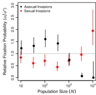
Sex has a short-term advantage in large populations. The data in Figure 1 document a long-term advantage to sexual reproduction at all population sizes. As a result, equilibrium sexual populations are expected to outcompete equilibrium asexual populations in head-to-head competition. However, the data in Figure 1 also indicate a short-term disadvantage associated with recombination load that is expected to impede both the origin and maintenance of sexual reproduction; a sexual mutant arising in an asexual population has an immediate disadvantage because it starts experiencing recombination load, whereas an asexual mutant arising in a sexual population has an immediate advantage because it stops experiencing recombination load.
Following the approach of Keightley and Otto (2006), we investigated the origin of sex by introducing a sexual mutant into equilibrium asexual populations. We similarly investigated the maintenance of sex by introducing an asexual mutant into equilibrium sexual populations. We then monitored the fate of the mutations until they were either fixed or lost from the population. We measured the fixation probability of the invading allele(u)relative to that of a neutral mutation (u∗ = 1/N) in at least5N replicate invasion trials at each population size.
In Figure 4, we show the effect of population size on these relative fixation probabilities,
u/u∗. At small population sizes, asexual modifiers invaded successfully more often than sexual modifiers, and this difference increased with population size until it achieved a maximum near N = 100. As population size increased further, the trend reversed so that sexual modifiers invaded successfully more often than asexual modifiers in large populations
(N >103; Figure 4). In the largest populations we tested (N = 104), sexual mutants invaded
asexual populations significantly more often than the neutral expectation (u/u∗ = 1.987,
n= 1.56×10⁵, p= 0.0005 by an exact binomial test). Although we report only the results of our Separate Sex implementation of sexual reproduction (see Materials and Methods, Reproductive mode) in Figure 4, we obtained qualitatively identical results using Recessive Sex (Figure 12A). Dominant Sex was neither able to invade nor to resist invasion by asexual modifiers (Figure 12B) for reasons we discuss in the Appendix.
Examining only the largest populations (N = 104), we explored the sensitivity of the
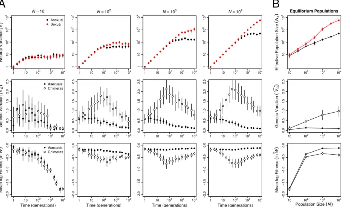
The short-term advantage of sex is caused by Hill-Robertson interference, not epistasis. In our invasion simulations, the immediate population genetic consequence of introducing sex into an asexual population is the break up of linkage disequilibrium (LD). Breaking up LD is expected to have two consequences. First, mean fitness will decline as beneficial combinations of alleles (positive LD) built up by selection are broken up; this selects against sex. Second, additive genetic variance in fitness will rise as negative LD built up by a combination of selection and genetic drift is broken up; this selects for sex. Figure 3 shows that both of these predictions are met for log fitness (lnW)for populations of 100 or more individuals.
If these immediate consequences of sex determined the invasion success of sexual modifiers, then we expect the increase in additive genetic variance to outweigh the decrease in mean fitness only in the largest populations (N = 104; Figures 4 and 12A). More precisely, higher
recombination is expected to evolve if the net advantage of eliminating LD is positive, i.e., if
∆lnW + ∆var(lnW) >0, where ∆ indicates the difference between a statistic in the real population and in a hypothetical population with the same allele frequencies but in linkage equilibrium (Barton, 1995). Figure 3B shows that at generation 104 the net advantage of
eliminating LD increases with population size and that ∆lnW + ∆var(lnW) > 0 for all asexual populations of 100 or more individuals (paired t-test: t≥3.417,df = 49,p≤0.0013).
In our model, the determinant of the short-term advantage of sex, negative LD, appears to have arisen from Hill-Robertson interference rather than from the negative epistasis that evolved in our simulations (Figure 1). Otto and Feldman (1997) predict the evolution of higher recombination rate only if the epistatic effects of mutations satisfy the following condition:
3ε∗+ (ε∗)2+ var(ε∗)<0
where ε∗ is a standardized epistasis coefficient (see Materials and Methods, Genetic architec-ture). None of the 50 populations summarized in Figure 1 (sexual or asexual) satisfied that condition at generation104. Thus, epistasis cannot explain the accumulation of negative LD in
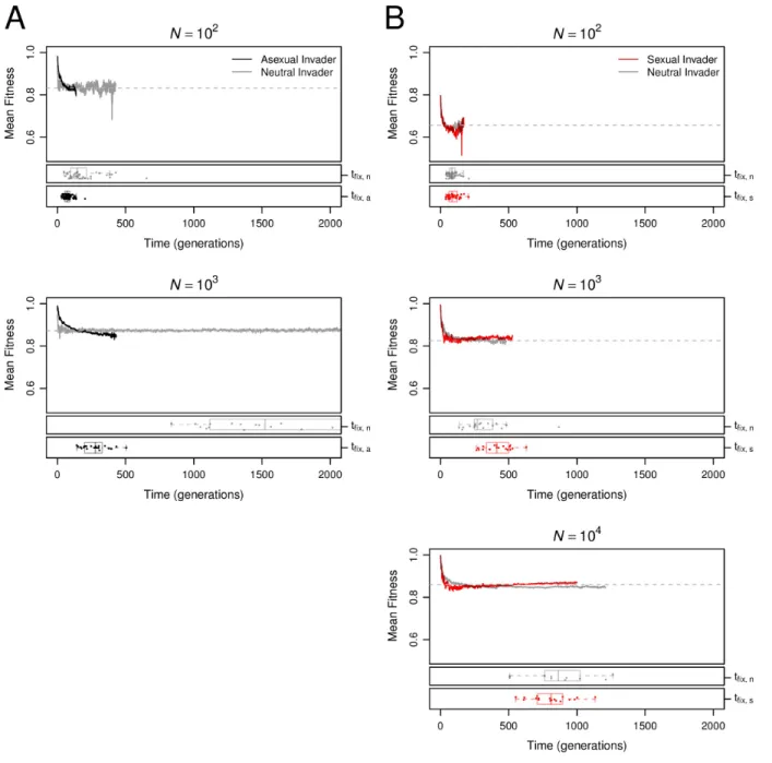
large asexual populations. Instead, it must have been caused by Hill-Robertson interference. Changes in the genetic architecture influence both the origin and maintenance of sex. Changes in the genetic architecture played a decisive role in generating a long-term advantage of sex (Figure 1). Here we investigate the role of changes in the genetic architecture in the short-term advantage of sex. To understand why the origin and maintenance of sex was favored only when population size was large, we investigated the mean fitness dynamics and fixation times of the sexual and asexual genotypes that successfully invaded (Figure 5). The immediate and short-term fitness consequences of mutations that alter reproductive mode were predictable from the dynamics of genetic architecture evolution. Asexual modifiers arising in sexual populations experienced an immediate fitness benefit due to the disappearance of recombination load and the advantageous genetic architecture (low Ud) they inherit from their sexual predecessors. The latter advantage decayed over time as asexual invaders evolved toward the asexual equilibrium. Most successful asexual invasions occurred quickly (Figure 5A, black points and boxplots), before the mean fitness of the invaders (Figure 5A, black lines) decayed below that of the resident sexual population (Figure 5A, dashed gray lines).
an advantageous genetic architecture (compare fitness trajectories in Figure 5B to Ud and
LR trajectories in Figure 1A). Successful sexual modifiers arose by chance in high fitness genomes, retained a higher fitness than the asexual mean for around 100 generations (Figure 5B, red lines) and hitchhiked to a relatively high frequency as a result (Figure 13). In populations of sizeN ≤100, the only sexual modifiers that fix appear to do so by hitchhiking quickly to fixation. In larger populations (N ≥103), the initial hitchhiking of sexual modifier mutations was critical to their invasion success because it enabled their persistence over the long timescale needed for the sexual invaders to evolve a higher mean fitness (Figure 5B, red lines) than that of the resident asexual population (Figure 5B, dashed gray lines). Similarly, population size (N) critically affected invasion probabilities because increasing
N increased the transit time (tfix) of new mutations to fixation (Figure 5, red and black
points and boxplots). Because the evolution of asexual disadvantages and sexual advantages is time-dependent, sexual resident populations and sexual invaders can be successful only if they persist long enough for these differences to evolve. Thus, our data reveal that the evolutionary success of sex at only the largest population sizes resulted from an interaction between the increase intfix and the differences in fitness dynamics between sexual and asexual
invaders (Figure 5).
Selection favors moderate recombination rates. Thus far, we have compared asexual reproduction to sexual reproduction with free recombination. However, we found that a small increase in recombination rate is favored even when sex is not (N = 103, compare
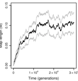
Figures 4 and 12A with 13), suggesting that “a little sex may go a long way” (Hurst and Peck, 1996) in our model. To investigate this phenomenon further, we allowed recombination rate to evolve in populations ofN = 103 individuals. Like our investigations of the evolution
length among 50 replicate simulations increased to λ≈0.1M within1.5×104 generations
(Figure 6). Thus, selection in the gene network model readily promoted the evolution of moderate, but not high, recombination rates in populations of N = 103 individuals.
DISCUSSION
We simulated evolution in a computational model of gene networks in order to determine how Hill-Robertson interference interacts with an evolving genetic architecture to impact the evolutionary origin and maintenance of sex. We found that the benefit of sex increased with population size, in agreement with earlier studies (Iles et al., 2003; Keightley and Otto, 2006; Gordo and Campos, 2008; Hartfield et al., 2010). Those studies identified Hill-Robertson interference as the principal cause of this pattern. We found that Hill-Robertson interference also played a role in our model in creating both a long-term and a short-term advantage of sex. But we also showed that the long- and short-term advantages of sex were determined by differences between sexual and asexual populations in the evolutionary dynamics of two properties of the genetic architecture,UdandLR. We next sought to quantify the contribution of Hill-Robertson interference to these dynamics.
We documented two differences between sexual and asexual populations that likely im-pacted the evolution of Ud. First, sexual populations uniquely experienced recombination load, LR. We know from previous work that selection to minimize LR, alone, results in increasing robustness to both recombination and mutation, loweringUd (Azevedo et al., 2006; Misevic et al., 2006; Gardner and Kalinka, 2006; Martin and Wagner, 2009; Lohaus et al., 2010). Second, asexual populations uniquely experienced Hill-Robertson interference that reduced Ne (Figure 3B). As in Keightley and Otto (2006), the reduction inNe increased with population size, N. At N = 100, Ne was reduced by 36% (from 72 to 46 individuals); at
N = 104,N
We quantified how these differences in the strength and efficiency of selection contributed to the equilibrium Ud in sexual and asexual populations in Figure 7. In that figure, we compare the equilibrium Ud between sexual and asexual populations of the same census size, N, and of the same effective size,Ne. Differences in Ud between populations of the same census size resulted from differences in both the strength and efficiency of selection, whereas differences in
Udbetween populations of the same effective size resulted from differences only in the strength of selection. In Figure 7 we see that the effect on Udof differences in the strength of selection (line b) decreased as population size increased, whereas the combined effect of differences in the strength and efficiency of selection (linea) was constant across the population sizes we examined. Thus, although differences in the strength of selection played a larger role than differences in the efficiency of selection at all the population sizes we examined, the relative contribution of selection efficiency grew with population size. In populations larger than 104
individuals, the reduced selection efficiency caused by Hill-Robertson interference may have eventually come to play the dominant role in determining Ud and, consequently, mean fitness in asexual populations.
Campos, 2008) ensured a perpetual decline in population mean fitness via Muller’s ratchet, regardless of population size, that would have been accelerated by Hill-Robertson interference in asexual populations. In our gene network model, Muller’s ratchet was eventually halted by an increasing frequency of compensatory mutations even at the smallest population sizes (Figure 1). As a result, direct effects of Hill-Robertson interference on advantages of sex in the gene network model were limited to populations that were small enough for Muller’s ratchet to operate over a wide fitness range.
One major difference between our results and those of earlier studies of Hill-Robertson interference, is that we observed only moderate advantages of sex. The long-term advantage of sex observed here (cWsex/Wcasex= 1.04 forN = 104) was substantial but may be considered
weak compared to the 2-fold cost experienced by many sexual species in nature. The short-term advantage was even weaker: it disappeared when we imposed as little as a 1% cost of sex (14). We note, however, that modifiers of sex generated smaller short-term advantages than modifiers of recombination (compare the N = 103 populations in Figures 4, 13 and 6), as has been observed in other models (Keightley and Otto, 2006).
et al., 2004; MacIsaac et al., 2006). In addition, we do not know the extent to which this yeast network is representative of other networks in nature. A strict comparison of connectivities between our networks and real biological networks is likely misleading because we only considered random gene networks, a pattern of connectivity that is probably unrealistic (Milo et al., 2002; Shen-Orr et al., 2002).
FIGURES 0.0 0.2 0.4 0.6 0.8 1.0
N=10
1 10 102
103 104 Asexual Sexual M e a n F it n e ss ( W ) 0.0 0.2 0.4 0.6 0.8 1.0
1 10 102
103 104 Asexual Sexual D e le te ri o u s M u ta ti o n R a te ( U d ) −20 −15 −10 −5 0 5
1 10 102
103 104 Asexual Sexual Epistasis ( ε *) 0.0 0.2 0.4 0.6 0.8 1.0
1 10 102 103 104
Asexual Sexual R e co m b in a ti o n L o a d ( LR )
Time(generations)
0.0 0.2 0.4 0.6 0.8 1.0
N=102
1 10 102
103 104 0.0 0.2 0.4 0.6 0.8 1.0
1 10 102
103 104 −20 −15 −10 −5 0 5
1 10 102
103 104 0.0 0.2 0.4 0.6 0.8 1.0
1 10 102 103 104
Time(generations)
0.0 0.2 0.4 0.6 0.8 1.0
N=103
1 10 102
103 104 0.0 0.2 0.4 0.6 0.8 1.0
1 10 102
103 104 −20 −15 −10 −5 0 5
1 10 102
103 104 0.0 0.2 0.4 0.6 0.8 1.0
1 10 102 103 104
Time(generations)
0.0 0.2 0.4 0.6 0.8 1.0
N=104
1 10 102
103 104 0.0 0.2 0.4 0.6 0.8 1.0
1 10 102
103 104 −20 −15 −10 −5 0 5
1 10 102
103 104 0.0 0.2 0.4 0.6 0.8 1.0
1 10 102 103 104
Time(generations)
0.0 0.2 0.4 0.6 0.8 1.0
10 102
103 104 Equilibrium Populations M e a n F it n e ss ( W ^) 0.0 0.2 0.4 0.6 0.8 1.0
10 102
103 104 D e le te ri o u s M u ta ti o n R a te ( Ud ^) −20 −15 −10 −5 0 5
10 102
103 104 Epistasis ( ε ^ *) 0.0 0.2 0.4 0.6 0.8 1.0
10 102 103 104
R e co m b in a ti o n L o a d ( LR ^)
PopulationSize(N)
A
B
0.0
0.2
0.4
0.6
0.8
1.0
PopulationSize(N)
E
q
u
ili
b
ri
u
m
M
e
a
n
F
it
n
e
ss
(
W
^)
10 102 103 104
0.0
0.2
0.4
0.6
0.8
1.0 A
Asexual Sexual
0.80
0.84
0.88
0.92
PopulationSize(N)
E
q
u
ili
b
ri
u
m
M
e
a
n
F
it
n
e
ss
(
W^
)
3×10² 103 3
×103 104 B
N=10
1 10 102
103 104 1 10 10 2 10 3 10 4 Asexual Sexual N e u tr a l V a ri a n ce ( V ) 0.0 0.5 1.0 1.5 2.0 2.5
1 10 102
103 104 G e n e ti c V a ri a ti o n ( V G ) Asexuals Chimeras −2.0 −1.5 −1.0 −0.5 0.0
1 10 102
103 104 Time (generations) M e a n lo g F it n e ss ( ln W ) Asexuals Chimeras
N=102
1 10 102
103 104 1 10 10 2 10 3 10 4 0.0 0.5 1.0 1.5 2.0 2.5
1 10 102
103 104 −2.0 −1.5 −1.0 −0.5 0.0
1 10 102
103
104
Time (generations)
N=103
1 10 102
103 104 1 10 10 2 10 3 10 4 0.0 0.5 1.0 1.5 2.0 2.5
1 10 102
103 104 −2.0 −1.5 −1.0 −0.5 0.0
1 10 102
103
104
Time (generations)
N=104
1 10 102
103 104 1 10 10 2 10 3 10 4 0.0 0.5 1.0 1.5 2.0 2.5
1 10 102
103 104 −2.0 −1.5 −1.0 −0.5 0.0
1 10 102
103
104
Time (generations)
Equilibrium Populations
10 102
103 104 10 10 2 10 3 10 4 E ff e ct ive P o p u la ti o n S ize ( N e ) 0.0 0.5 1.0 1.5 2.0 2.5
10 102
103 104 G e n e ti c V a ri a ti o n ( V G ) −2.0 −1.5 −1.0 −0.5 0.0
10 102
103 104 M e a n lo g F it n e ss ( ln W ^ )
PopulationSize (N)
A
B
Figure 3: Robertson interference affected asexual populations of all sizes. (A) Hill-Robertson interference depressed variance at a neutral locus (V) in asexual (black) compared to sexual (red) populations (top row). The LD that accumulated in asexual populations also decreased genetic variance in log fitness, var(lnW), and increased mean log fitness, lnW. Data in the middle and bottom rows compare these metrics in the real asexual populations (closed circles) and populations of chimeras with the same allele frequencies but no LD (open
circles). (B) Means of each metric at generation 104. Effective population size (N
0.0
0.5
1.0
1.5
2.0
2.5
3.0
PopulationSize(N)
Relativ
e Fixation Probability (
u
u
*)
10 102
103
104
Asexual Invasions Sexual Invasions
Figure 5: Changes in the genetic architecture influence both the origin and maintenance of sex. We monitored the fixation and loss of asexual mutants introduced into equilibrium sexual populations (black lines, panel A), of sexual mutants introduced into equilibrium asexual populations (red lines, panel B), and of neutral mutants introduced into both sexual and asexual populations (solid gray lines, panels A and B, respectively). Lines show the evolution of mean fitness among invading mutants, averaged over at least 10 successful invasions. The equilibrium mean fitness of the populations being invaded is represented by a gray dashed line across each plot. Points and corresponding boxplots shown at the bottom of each plot indicate the time of fixation for individual neutral (tfix,n), sexual (tfix,s), or asexual (tfix,a)
0.00
0.05
0.10
0.15
Time (generations)
Map length (M)
0 1×10⁴ 2 ×10⁴ 3
×104
Figure 6: Evolution of the recombination rate under recurrent mutation at the recombination modifier locus. Black and gray lines show the change in mean and 95% confidence interval, respectively, of the genome map length (i.e. mean crossover probability) over time. Data are from 50 replicates initiated with the equilibrium asexual populations of size N = 103 shown in Figure 1.
0.05
0.10
0.15
0.20
0.25
0.30
PopulationSize(N or Ne)
D
e
le
te
ri
o
u
s
M
u
ta
ti
o
n
R
a
te
(
U
d)
10 102
103
104
a b
Figure 7: Hill-Robertson interference explains part of the difference in equilibrium Ud between sexual (red) and asexual (black) populations. Equilibrium values of the genome-wide deleterious mutation rate Ud versus census population sizeN (open circles, replotted from Figure 1) and versus effective population size Ne (closed circles). Lines are best fit linear models obtained separately using N (dashed lines) or Ne (solid lines) as a dependent variable together with reproductive mode. The total difference inUd exhibited by sexual and asexual populations of census size N = 104 (gray line a) is attributable to both differences in the strength and efficiency of selection acting on genetic architecture. The difference in
0.0 0.2 0.4 0.6 0.8 1.0
N=10
1 10 102
103 104 Asexual Sexual M e a n F it n e ss ( W ) 0.00 0.05 0.10 0.15 0.20
1 10 102
103 104 Asexual Sexual P ro p o rt io n B e n e fi ci a l ( pb ) 0.4 0.5 0.6 0.7 0.8 0.9 1.0
1 10 102
103 104 Asexual Sexual P ro p o rt io n N e u tr a l ( pn ) 0.00 0.05 0.10 0.15 0.20
1 10 102 103 104
Asexual Sexual P ro p o rt io n D e le te ri o u s ( pd ) 0.0 0.1 0.2 0.3 0.4 0.5
1 10 102 103 104
Asexual Sexual P ro p o rt io n L e th a l ( pl ) −0.5 −0.4 −0.3 −0.2 −0.1 0.0
1 10 102 103 104
Asexual Sexual M e a n D e le te ri o u s E ff e ct ( s )
Time(generations)
0.0 0.2 0.4 0.6 0.8 1.0
N=102
1 10 102
103 104 0.00 0.05 0.10 0.15 0.20
1 10 102
103 104 0.4 0.5 0.6 0.7 0.8 0.9 1.0
1 10 102
103 104 0.00 0.05 0.10 0.15 0.20
1 10 102 103 104
0.0 0.1 0.2 0.3 0.4 0.5
1 10 102 103 104
−0.5 −0.4 −0.3 −0.2 −0.1 0.0
1 10 102 103 104
Time(generations)
0.0 0.2 0.4 0.6 0.8 1.0
N=103
1 10 102
103 104 0.00 0.05 0.10 0.15 0.20
1 10 102
103 104 0.4 0.5 0.6 0.7 0.8 0.9 1.0
1 10 102
103 104 0.00 0.05 0.10 0.15 0.20
1 10 102 103 104
0.0 0.1 0.2 0.3 0.4 0.5
1 10 102 103 104
−0.5 −0.4 −0.3 −0.2 −0.1 0.0
1 10 102 103 104
Time(generations)
0.0 0.2 0.4 0.6 0.8 1.0
N=104
1 10 102
103 104 0.00 0.05 0.10 0.15 0.20
1 10 102
103 104 0.4 0.5 0.6 0.7 0.8 0.9 1.0
1 10 102
103 104 0.00 0.05 0.10 0.15 0.20
1 10 102 103 104
0.0 0.1 0.2 0.3 0.4 0.5
1 10 102 103 104
−0.5 −0.4 −0.3 −0.2 −0.1 0.0
1 10 102 103 104
Time(generations)
0.0 0.2 0.4 0.6 0.8 1.0 Equilibrium Populations
10 102
103 104 M e a n F it n e ss ( W ^) 0.00 0.05 0.10 0.15 0.20
10 102
103 104 P ro p o rt io n B e n e fi ci a l ( pb ^) 0.4 0.5 0.6 0.7 0.8 0.9 1.0
10 102
103 104 P ro p o rt io n N e u tr a l ( pn ^) 0.00 0.05 0.10 0.15 0.20
10 102 103 104
P ro p o rt io n D e le te ri o u s ( pd ^) 0.0 0.1 0.2 0.3 0.4 0.5
10 102 103 104
P ro p o rt io n L e th a l ( pl ^) −0.5 −0.4 −0.3 −0.2 −0.1 0.0
10 102 103 104
M e a n D e le te ri o u s E ff e ct ( s ^)
PopulationSize(N)
A
B
Figure 8: Evolution of the distribution of mutation effects. (A) Change in mean fitness (replotted from Figure 1), proportions of mutations (pb, pn, pd, pl) that are beneficial (s >0),
0.80
0.85
0.90
0.95
1.00
Mean
Fitness
(
W
^ )
0.1 1.0 Asexual Sexual
0.00
0.10
0.20
0.30
Proportion
Deleterious
Mutations
(
pd ^+ pl ^)
0.1 1.0
0.00
0.04
0.08
Recombination
Load
(
LR
^ )
0.1 1.0
100
500
2000
10000
Eff
e
cti
v
e
Po
pula
ti
on
S
iz
e
(
Ne
)
0.1 1.0
0
5
10
15
Relativ
e Fixation Probability
(
u
u
*)
0.1 1.0
MutationRate(U)
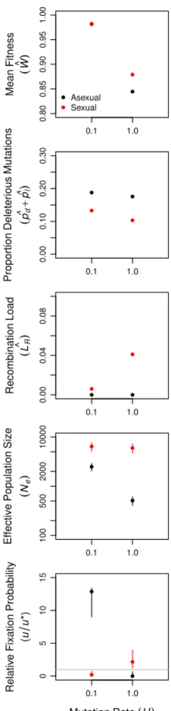
Figure 9: Equilibria and invasion probabilities for large populations (N = 104) at low (U = 0.1) and high (U = 1) genome-wide mutation rates. The top 4 panels show means and 95% confidence intervals for asexual (black) and sexual (red) populations at generation
0.0 0.2 0.4 0.6 0.8 1.0
0.02 0.05 0.08
Asexual Sexual M e a n F it n e ss ( W ^) 0.0 0.2 0.4 0.6 0.8 1.0
0.02 0.05 0.08
D e le te ri o u s M u ta ti o n R a te ( Ud ^) 0.0 0.1 0.2 0.3 0.4 0.5
0.02 0.05 0.08
R e co m b in a ti o n L o a d ( LR ^) 100 200 500 1000 2000
0.02 0.05 0.08
E ff e ct ive P o p u la ti o n S ize ( Ne ) 0.0 0.5 1.0 1.5 2.0 2.5 3.0
0.02 0.05 0.08
Relativ
e Fixation Probability (
u
u
*)
Connectivity(c)
Figure 10: Network connectivity (c) impacts the long- and short-term advantages of sex. The top 4 panels show means and 95% confidence intervals for asexual (black) and sexual (red) populations at generation 104, after populations at each connectivity had achieved an
equilibrium in all metrics. Dashed gray lines indicate the 95% confidence intervals after the first generation in panels 1–3 and the census size of all populations (N = 103) in panel 4.
0.0
0.5
1.0
1.5
2.0
2.5
3.0
Recessive Sex
PopulationSize(N)
Relativ
e Fixation Probability (
u
u
*)
10 102 103 104
A Asexual Invasions Sexual Invasions
0
5
10
15
20
25
30
Dominant Sex
PopulationSize(N)
Relativ
e Fixation Probability (
u
u
*)
10 102
103 104 B Asexual Invasions
Sexual Invasions
Figure 11: Relative fixation probabilities (u/u∗)of recessive and dominant modifiers of sex. Individual asexual (black) or sexual (red) modifier mutations were introduced into equilibrium sexual or asexual populations, respectively, at an initial frequency of 1/N. Populations were then allowed to evolve using either the Recessive Sex (A) or Dominant Sex (B) reproductive mode (see Materials and Methods, Reproductive mode). In both cases, frequencies of the modifier mutations were monitored until the mutations were either fixed or lost. Data are the proportion of fixations (u)divided by the neutral expectation(u∗ = 1/N)and95%confidence intervals based on ≥5N replicate invasion trials for each population size(N).
0.0
0.5
1.0
1.5
2.0
PopulationSize(N)
Relativ
e Fixation Probability (
u
u
*)
10 102
103
Figure 12: Relative fixation probabilities(u/u∗)of a modifier of recombination. The modifier mutation increased the genetic map length from λ = 0 to 0.05 M and acted additively. Individual modifier mutations were introduced into equilibrium asexual populations, at an initial frequency of 1/N. Populations were then allowed to evolve. Frequency of the modifier mutation was monitored until it was either fixed or lost. Data are the proportion of fixations
(u) divided by the neutral expectation (u∗ = 1/N) and 95%confidence intervals based on
0 100 200 300 400 500 600 −6 −4 −2 0 2 4 6 Time (generations) logit ( f )
N=102
0 200 400 600 800
−6 −4 −2 0 2 4 6 Time (generations) logit ( f )
N=102
0 100 200 300 400 500 600
−6 −4 −2 0 2 4 6 Time (generations) logit ( f )
N=103
0 200 400 600 800
−6 −4 −2 0 2 4 6 Time (generations) logit ( f )
N=103
0 200 400 600 800
−6 −4 −2 0 2 4 6 Time (generations) logit ( f )
N=104
A
B
0
10
20
30
40
CostofSex(C)
Relativ
e Fixation Probability (
u
u
*)
1.00 1.01 1.02
Asexual Invasions Sexual Invasions
Figure 14: Costly sex does not evolve. Individual asexual (black) or sexual (red) modifier mutations were introduced, respectively, into equilibrium sexual or asexual populations of
N = 104 individuals at an initial frequency of1/N. Asexually produced offspring have fitness
Wasex = W (Equation 2). Sexually produced offspring have fitness Wsex = W/C, where