Continuous Medial Models in Two-Sample
Statistics of Shape
by
Timothy B. Terriberry
A dissertation submitted to the faculty of the University of North Carolina at Chapel Hill in partial fulfillment of the requirements for the degree of Doctor of Philosophy in the Department of Computer Science.
Chapel Hill 2006
Approved by:
Guido Gerig, Advisor Sarang C. Joshi, Reader Stephen M. Pizer, Reader
c 2006
ABSTRACT
TIMOTHY B. TERRIBERRY: Continuous Medial Models in Two-Sample Statistics of Shape.
(Under the direction of Guido Gerig.)
In questions of statistical shape analysis, the foremost is how such shapes should be represented. The number of parameters required for a given accuracy and the types of deformation they can express directly influence the quality and type of statistical inferences one can make. One example is a medial model, which represents a solid object using a skeleton of a lower dimension and naturally expresses intuitive changes such as “bending”, “twisting”, and “thickening”.
In this dissertation I develop a new three-dimensional medial model that allows continuous interpolation of the medial surface and provides a map back and forth be-tween the boundary and its medial axis. It is the first such model to support branching, allowing the representation of a much wider class of objects than previously possible using continuous medial methods.
A measure defined on the medial surface then allows one to write integrals over the boundary and the object interior in medial coordinates, enabling the expression of important object properties in an object-relative coordinate system. I show how these properties can be used to optimize correspondence during model construction. This improved correspondence reduces variability due to how the model is parameterized which could potentially mask a true shape change effect.
ACKNOWLEDGMENTS
No scientific progress is possible without standing on the shoulders of giants, and it was my good fortune to have a group of professors and fellow students filled with many such shoulders. As the references will attest, I have made much use of their ideas, and this dissertation would not have been possible without them. I can think of no greater compliment one could pay a fellow scientist.
But there is another group of people who are essential to any student’s progress: the accountants, administrators, assistants, and secretaries who keep the department running. And so, I extend my sincerest gratitude to Delphine Bull, Katrina Coble, Kelli Gaskill, Janet Jones, Sandra Neely, Deb O’Connor, Tammy Pike, and Karen Thigpen. These are the folks who make sure we get from here to there.
Contents
List of Figures xi
List of Tables xiii
1 Introduction 1
1.1 Motivation and Goals . . . 1
1.1.1 A Continuous Medial Model . . . 2
1.1.2 Model Fitting With Explicit Correspondence Optimization . . . 3
1.1.3 Nonlinear Hypothesis Testing . . . 4
1.1.4 Thesis and Claims . . . 5
1.1.5 Overview . . . 5
2 Medial Properties 7 2.1 An Overview of the Medial Axis . . . 7
2.2 Shape Analysis Using the Medial Axis . . . 13
2.2.1 M-reps . . . 15
2.3 Mathematical Background . . . 18
2.3.1 Whitney Stratified Sets. . . 18
2.3.2 Skeletal Sets and Radial Vector Fields . . . 20
2.3.3 The Blum Medial Axis as a Skeletal Structure . . . 25
2.3.4 Geometry of the Boundary . . . 27
2.3.5 Integrals Over Skeletal Structures . . . 31
3 A Continuous Medial Model 37 3.1 Catmull-Clark Subdivision on the Medial Axis . . . 38
3.1.1 Ordinary Corner-Free Boundary . . . 39
3.2 Edge Patches . . . 46
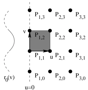
3.2.1 Solving forru(0, v) . . . 48
3.2.2 The Complete Control Curve . . . 50
3.2.3 Sympathetic Overfolding . . . 51
3.3 Branch Curve Patches . . . 56
3.3.1 Satisfying Branch Conditions Away From Fin Creation Points . 58 3.3.2 Satisfying Edge and Branch Conditions at a Fin Creation Point 59 3.3.3 Transition Region . . . 63
3.4 Summary and Conclusion . . . 64
4 Model Fitting With Explicit Correspondence Optimization 67 4.1 Approximating Medial Integrals . . . 69
4.1.1 Sampling the Medial Axis . . . 69
4.1.2 Moment Integrals . . . 72
4.1.3 Estimating Volume Overlap . . . 73
4.2 Single-Subject Model Fitting . . . 75
4.2.1 Template Alignment . . . 75
4.2.2 Model Deformation . . . 76
4.2.3 Local Nonlinear Optimization . . . 82
4.2.4 Constrained Optimization . . . 86
4.2.5 Results. . . 90
4.3 Population-Based Model Fitting . . . 93
4.3.1 The Objective Function for Correspondence . . . 98
4.3.2 Parameterizing the Correspondence Optimization . . . 100
4.3.3 Results. . . 102
4.4 Conclusion . . . 103
5 Nonlinear Hypothesis Testing 106 5.1 Introduction . . . 107
5.1.1 A Metric Space for M-reps . . . 109
5.1.2 One-sample Statistics in Nonlinear Spaces . . . 110
5.1.3 Two-sample Statistics . . . 112
5.2 Multivariate Permutation Tests . . . 113
5.2.1 The Univariate Case . . . 113
5.2.2 Partial Tests. . . 114
5.2.4 Relation to Other Testing Procedures . . . 118
5.3 Experimental Data and Results . . . 119
5.4 Conclusion . . . 122
6 Conclusion 125
A Computing U± and Srad in Three Dimensions 130
A.1 Derivatives of the Edge Control Curve . . . 134
B Derivatives for Optimizing U± and Srad 137
B.1 Derivatives of the Edge Control Curve . . . 140
List of Figures
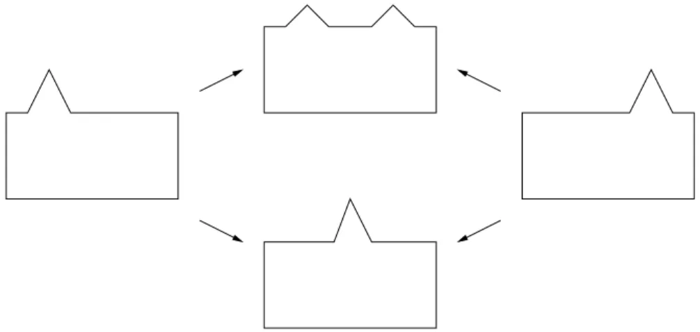
1.1 Different notions of correspondence . . . 4
2.1 Examples of the medial axes of some generic shapes . . . 10
2.2 The generic local singular structures for the Blum medial axis . . . 11
2.3 The Whitney umbrella . . . 22
2.4 An example of overfolding . . . 28
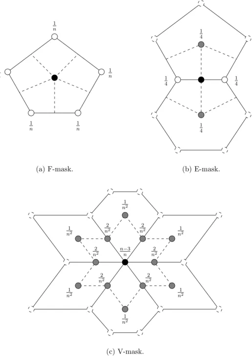
3.1 Catmull-Clark subdivision masks . . . 40
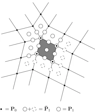
3.2 Control points around an extraordinary vertex . . . 43
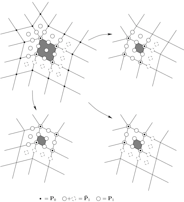
3.3 Subdivision near an extraordinary vertex . . . 44
3.4 The control curve on an edge patch . . . 47
3.5 An example of sympathetic overfolding . . . 52
3.6 An example of a pair of edge patches . . . 55
3.7 Two close-ups of the right portion of an edge patch . . . 56
3.8 The cross-section of a branch curve . . . 58
3.9 A fin point example . . . 63
4.1 Population-based correspondence optimization . . . 68
4.2 The best fit for the deformed ellipsoids . . . 92
4.3 The worst fit for the deformed ellipsoids . . . 92
4.4 An average fit for the deformed ellipsoids . . . 92
4.5 Surface errors for the deformed ellipsoids . . . 93
4.7 The worst fits for the caudate data . . . 94
4.8 Average fits for the caudate data . . . 95
4.9 Surface errors for the caudate data . . . 95
4.10 Clustering of corresponding points for the deformed ellipsoids . . . 103
4.11 Clustering of corresponding points for the caudate data . . . 104
5.1 Lateral ventricle examples . . . 108
5.2 Example data and test statistics . . . 116
5.3 Empirical distribution of our example . . . 118
5.4 Genetic similarity results for local tests . . . 122
List of Tables
4.1 Surface errors for the deformed ellipsoids . . . 91
4.2 Surface errors for the caudate data . . . 93
Chapter 1
Introduction
. . . it appears to me possible. . . to reconstruct the skeleton of the one from our knowledge of the skeleton of the other, under the guidance of the same correspondence as is indicated in their external configuration.
(Thompson, 1917)
1.1
Motivation and Goals
D’Arcy Thompson’s words, written the better part of a century ago to describe his hand-made sketches of two different species of fish, eloquently sum up the goal of this work. This dissertation seeks to place a mathematical formalism and computational framework behind the process Thompson describes, and in so doing develops several new tools for the understanding of populations of shapes.
Given the widespread use of medical imaging, there is a great need for techniques to find and analyze the objects in them, a process greatly aided by an a priori under-standing of the variability of shapes between subjects and over time. These can be used for treatment planning: for visualizations of minimally-invasive surgery (possibly even while the operation is in progress) or radiation therapy, which aims to target tumors without killing the surrounding healthy tissue.
ways, such as “bending”, “twisting”, or “thickness”, helps researchers to understand the disease process. Furthermore, these tools help in understanding the effects of vari-ous drugs used to treat these diseases. They can also be used to analyze the processes of growth and early development.
However, describing shapes in these terms requires nonlinear models to capture what are inherently nonlinear processes. These models require new statistical methods that generalize those developed for linear spaces to nonlinear ones.
1.1.1
A Continuous Medial Model
One particularly powerful class of shape representations aremedial representations, or m-reps. As a kind of skeleton, their description carries with it information about the solid shape that boundary descriptions do not and naturally decomposes into figural parts, connected at branches where multiple parts meet. They also naturally describe the intuitive types of shape change listed above.
The medial geometry provides an intrinsic link between the boundary and the me-dial axis, which allows one to use the appropriate representation for the desired analysis task. However, there are a number of limitations with current m-rep models. In the discrete version (Pizer et al., 1999) the connection with the boundary is tenuous: the link is given only at a coarse set of discrete points and the interpolation given by (Thall, 2004) to recover a dense sampling does not respect the intrinsic medial geometry. More recent work on interpolation that does respect this geometry shows a promising alter-native (Han et al., 2006), but it sacrifices the uniqueness of the representation, requires expensive numerical integration, and in the end only approximately interpolates the original discrete model.
An alternative approach, cm-reps, consider the problems of designing a discrete computer representation and computing its associated continuous mathematical repre-sentation together as a coupled system. However, generalizations to three dimensions require an infinite number of boundary conditions to be satisfied. Existing techniques for enforcing them are limited to a single figure (Yushkevich, 2003; Yushkevich et al., 2005), and thus can represent only a limited class of objects.
This technique allows the creation of the first continuous medial model that supports branching in three dimensions.
1.1.2
Model Fitting With Explicit Correspondence
Optimiza-tion
The link between medial geometry and the geometry of the boundary provided by a continuous medial representation allows many operations on the boundary or interior of the shape to be expressed in terms of integrals in object-relative, medial coordinates. This forms the basis for the model-fitting framework outlined in Chapter4. A method of sampling the continuous medial axis is given, and this sampling is used to numerically approximate medial integrals. Several examples of such integrals include the compu-tation of volume overlap, which is a metric used to evaluate goodness-of-fit, as well as moments up through second order, which are used to initialize the fitting process by aligning a template to the target shape. The fitting process itself is governed by the constrained optimization of an objective function, also given by a medial integral, over several scales in succession. This chapter derives such multi-scale objective functions for both voxelized binary images and also triangulated surface meshes.
Finally, it shows how medial integrals can be used to tackle the problem of correspon-dence. An inherent problem in any shape representation used for statistical analysis, one must ensure that the parameters of the representation in some sense control the “same” features of the resulting shape. Otherwise, noise in the parameterization can overwhelm the size of any shape change effect, reducing or eliminating the power of the tests.
Figure 1.1: Different notions of correspondence can lead to different meanings of the average of a shape, as well as other statistics.
These methods of determining correspondence often focus solely on the boundary, since in many medical imaging modalities the interior of objects are relatively uniform in appearance and their features are poorly localized. Because a continuous represen-tation affords an explicit link between the boundary and the medial locus, the implicit correspondence given by the parameterization of the latter is optimized to match an explicit correspondence given on the former. Any number of existing methods, as well as future, problem-specific ones, can determine the correspondence, providing increased flexibility to adapt to the problem at hand.
1.1.3
Nonlinear Hypothesis Testing
1.1.4
Thesis and Claims
Thesis: Nonlinear growth and deformation of biological objects requires nonlinear shape models to effectively characterize these processes. A nonlinear hypothesis test based on multivariate permutation tests provides an effective means of detecting and localizing their effects between groups. A continuous medial model, which describes this variation in a natural way, can be used to effectively represent these shapes. The geometric link between the medial axis and the boundary such a model provides can be used to optimize the correspondence across a population of objects, reducing parameterization noise to increase the power of statistical tests.
The main contributions are
1. A novel “control curve” formulation capable of enforcing first- and second-order boundary conditions at the edges of subdivision surfaces.
2. A new continuous medial model based on this formulation, the first such model capable of representing branching in three dimensions.
3. A method of approximating medial integrals driven by a uniform sampling of these continuous models.
4. Applications of these medial integrals. These include computing volume overlap to evaluate goodness-of-fit and computing second-order moments to align models to a common position, orientation and scale.
5. A multi-scale model fitting framework utilizing a highly constrained multivariate nonlinear optimization to fit these models to a target shape.
6. A new correspondence optimization method that works in tandem with the model fitting process to produce a group of models with a common parameterization. 7. A novel nonlinear hypothesis test for m-reps, which simultaneously considers all
of the parameters of the shape model.
1.1.5
Overview
correspondence, Riemannian geometry, and hypothesis testing are embedded directly in the chapters that require them. The next three chapters form the bulk of the disserta-tion, covering each of the three topics outlined above. Chapter3defines the new medial representation, and shows how it can model branching in three dimensions. Chapter4
Chapter 2
Medial Properties
We are apt to think of mathematical definitions as too strict and rigid for common use, but their rigour is combined with all but endless freedom. . . . By means of these large limitations, by this controlled and regulated freedom, we reach through mathematical analysis to mathematical synthe-sis. . . as for instance, when we learn that, however we hold our chain, or however we fire our bullet, the contour of the one or the path of the other is always mathematically homologous.
(Thompson, 1917)
This chapter outlines the properties and mathematics of the Blum medial axis as it has been used in research up to this point. Additional background material, being fairly localized in its application, is not presented here, but rather directly in the chapters that require it. Chapter 3 contains a review of Catmull-Clark subdivision surfaces, Chapter 4 describes some necessary nonlinear optimization techniques, and Chapter5
briefly reviews hypothesis testing and one-sample statistics in Riemannian symmetric spaces.
2.1
An Overview of the Medial Axis
Giblin and Kimia, 2004). Extending the definition to higher dimensions is straightfor-ward; doing so, (Damon, 2003; Damon, 2004) provides an analysis of the differential geometry in any dimension.
A precise definition may be formulated in several different, equivalent ways. One approach is in terms of a maximally inscribed ball.
Definition 2.1 Given a point m ∈Rn, a closed ball of radius r around m is the set
Br(m) ={x∈Rn :kx−mk ≤r}.
Definition 2.2 Given a closed, connected set Ω⊆Rn, a maximally inscribed ball
in Ω is a closed ball B ⊆Ω such that there is no closed ball B0 with B (B0 ⊆Ω. Definition 2.3 The Blum medial axis of a closed, connected set Ω⊆Rn is the set
M ={m ∈Rn :B
r(m) is maximally inscribed for some r}.
By itself, the Blum medial axis is insufficient to describe the shape of an object, as many objects may have the same medial axis. Thus, we also define an augmented structure.
Definition 2.4 The augmented Blum medial axis of a closed, connected set Ω⊆ Rn is the set M={(m, r)∈Rn×R≥0 :Br(m) is maximally inscribed}.
Thisis a complete description of the object. The set Ω may be recovered from M—at least in an abstract mathematical sense—as the union of the maximally inscribed balls. Authors in various fields have used the termsmedial scaffold,central set,internal medial locus, and others to refer to the augmented or unaugmented versions of the medial axis. Where the notation,M orM, makes the definition in question clear, this dissertation will omit the word “augmented”.
There are many equivalent, alternative ways to define the medial axis. One is based on thesymmetry set, which replaces maximally inscribed balls withbitangent spheres: closed balls that are tangent to the boundary B = ∂Ω of the object in (at least) two different places (Giblin and Brassett, 1985). This requires that the object have a well-defined tangent plane (almost) everywhere on its boundary, which in practice is a reasonable restriction. The full symmetry set is larger than the medial axis, containing the closure of all such bitangent spheres. The closure is necessary to include points like the end points (such as the A3 point in Figure 2.1(a)), which in the generic case
A third approach defines the medial axis as the shocks of the grassfire flow (Blum, 1973). The analogy likens the object to a field of grass whose entire boundary is simultaneously set ablaze. As the fire’s front spreads from the boundary at a uniform speed, it meets at places called shocks from two different directions at once, where it extinguishes itself. The augmented medial axis can then be defined as the location of the shocks together with the times when they were formed. This can be modeled by the differential equation
∂C
∂t =−αN . (2.1)
HereC denotes the location of the fire front at time t, N is the outward facing normal to the front, and α is a positive constant controlling the speed of the flow. This analytic approach was shown to be equivalent to the geometric definition by (Calabi and Hartnett, 1968).
A fourth approach is based on the Euclidean distance transform.
Definition 2.5 The signed Euclidean distance transformof a set Ωis the func-tion DΩ :Rn →R≥0 given by
DΩ(x) =
infx0∈Ωd(x, x0), x6∈Ω
−infx0∈
Rn\Ωd(x, x0), x∈Ω
, (2.2)
where d(·,·) is the Euclidean distance function.
Then the medial axis is given by the “ridges” of the graph of DΩ that lie inside Ω.
These are given by the closure of the set of singular points, where two distinct points x0 ∈ B both give the infimum in (2.2).
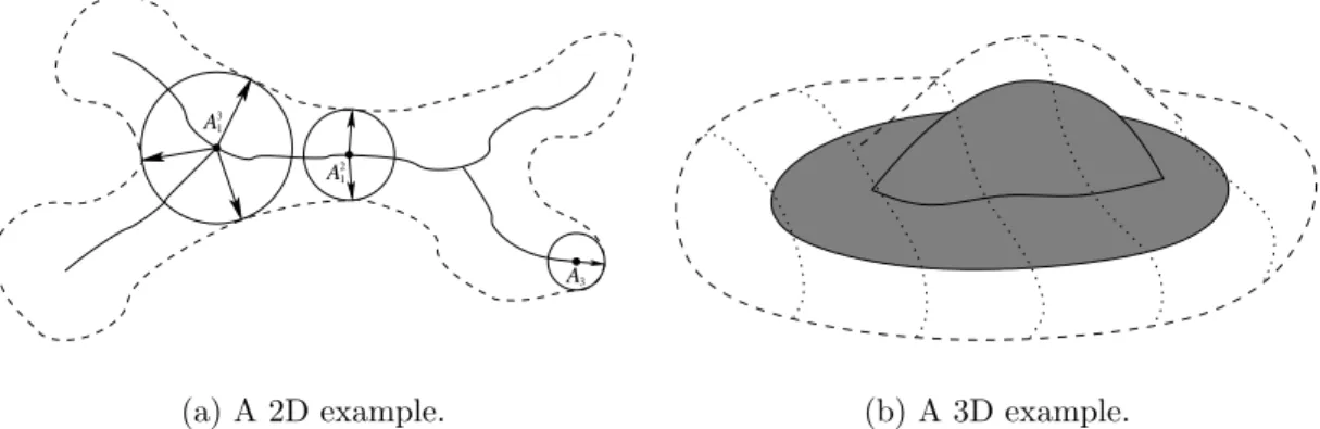
It is helpful to get a mental picture of what the set M looks like, so Figure 2.1
illustrates an example for two and three dimensions. In two dimensions, the centers of the inscribed balls form a set of curves that meet atbranch points. In three dimensions, they are typically a set of 2D manifolds with boundary, calledsheets, which meet along branch curves. We will call the boundary of these sheets edges and points along them edge points, to avoid confusion with the boundary of the object, B. The vectors from the center of a ball to the points of tangency on the boundary have been called in various places spokes, sails, or oars. In this work we shall adopt the term spokes.
A3 1
A2 1
A3
(a) A 2D example. (b) A 3D example.
Figure 2.1: Examples of the medial axes of some generic shapes. Most points are smooth points, like point A2
1, with a bitangent circle. Examples of singular points in
2D include branch points, like point A31, with a tritangent circle, and edge points, like point A3, with an osculating circle. TheAnk notation is explained in detail in the text.
give such a classification for two dimensions, while (Giblin and Kimia, 2004) give a rigorous classification in three dimensions for a generic boundary. We shall adopt the notation of the latter, where each pointAnk is classified by the number of unique points of tangency of the maximally inscribed ball with the boundary (n), along with the order of contact (Ak). The only two possible orders of contact of a maximally inscribed
ball Br(m) at a point on the boundary x∈ B are
• A1 contact: Br(m) is tangent toB atx.
• A3 contact: Br(m) is tangent toBatx,ris one of the principal radii of curvature
of B at x, and the corresponding principal curvature is a local extremum (also called aridge point of B).
There are three other orders of contact,A2,A4, andD4, but at such places the boundary
must penetrate the surface of the ball, so it can never be maximally inscribed. Thus no ball on the medial axis will make such contact withB (but points on the symmetry set might).
This notation is extended directly for contact at more than one point, e.g.,A1A1 =
A2
1 is normal bitangent contact. In 2D, the possible generic cases are
1. Curves (one dimensional manifolds) of A2
1 points.
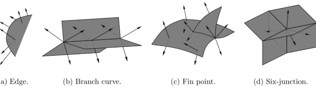
(a) Edge. (b) Branch curve. (c) Fin point. (d) Six-junction.
Figure 2.2: The generic local singular structures for the Blum medial axis in R3.
These can be extended to three dimensions, where two additional cases arise: 1. Sheets (two dimensional manifolds) of A2
1 points.
2. A3
1 branch curves (one dimensional manifolds), where threeA21 sheets meet.
3. A3 edge curves (one dimensional manifolds), where an A21 sheet ends.
4. A1A3 fin points (zero dimensional manifolds), where an A31 branch curve ends.
5. A4
1 six-junction points (zero dimensional manifolds), where fourA31 branch curves
connecting sixA2
1 sheets meet.
These are illustrated in Figure 2.2.
In general, if we want to restrict our attention to genus zero objects—those home-omorphic to the n-dimensional sphere—then we require some restrictions on how the strata are connected to each other. For example, in 2D, it is enough to require that the (undirected) graph of the connections between the medial sheets forms a tree (e.g., con-tains no cycles). In higher dimensions, this is still sufficient, but not necessary. Rather, the situation is more complex. Not only may the connectivity graph no longer be a tree, but neither is it sufficient to simply describe which sheets are connected to each other. Rather, how they are connected along branch curves also becomes important. A complete characterization of the topologies of the medial axes of genus zero objects in 3D is given by (Damon, 2005b).
medial axis of a given shape. Different approaches are based on Voronoi skeletons (Sz´ekely et al., 1994; Sheehy et al., 1996; Sherbrooke et al., 1996;Amenta et al., 2001; Leymarie and Kimia, 2003), morphological thinning (Borgefors et al., 1999;Manzanera et al., 1999), core tracking (Pizer et al., 1998), and shock detection (Kimia et al., 1990; Siddiqi et al., 2002;Torsello and Hancock, 2006); see (Pizer et al., 2003) for an overview and comparison of most of these. However, the problem is in general ill-posed, as small perturbations in the boundary of the shape can introduce large branches on the medial axis, and the branching structure can vary drastically between similar shapes. It is not clear how meaningful statistics can be performed over shape models with such widely varying topology.
This fundamental difficulty has led researchers to a different approach (Golland et al., 1999; Pizer et al., 1999). In a sense that will be made precise in Section 2.3.5, the effect of these extra branches on the actual shape is very small. Thus, instead of trying to extract the medial axis corresponding to an object, we start with a medial axis with a fixed branching topology and deform it until it matches our target object within a desired tolerance. Starting from a desired tolerance, (Styner et al., 2003) give an automatic method for computing a suitable topology for a collection of objects based on pruning their Voronoi diagrams. The specific incorporation of tolerance defines the scale of the features being modeled, and varying it produces multi-scale methods with all of their advantages.
2.2
Shape Analysis Using the Medial Axis
As a descriptor ofshape, the medial axis can be used to provide a detailed quantitative and qualitative analysis that simpler object descriptors, such as volume, surface area, pose, etc., cannot. To this end, the medial axis has been applied to a number of shape analysis tasks by various researchers, as summarized below. The medial axis is certainly not the only shape descriptor found in the literature. Others include landmarks and point distribution models (PDMs) (Cootes et al., 1992; Bookstein, 1997), spherical harmonics (SPHARMs) (Brechb¨uhler et al., 1995; Shenton et al., 2002), deformation fields (e.g., from a standard template or atlas) (Christensen et al., 1993; Martin et al., 1994;Machado and Gee, 1998), or distance transforms (Golland et al., 2002;Leventon et al., 2000). A complete discussion of all of these is beyond the scope of this chapter.
A medial representation, however, has a number of compelling features. Their branching topology provides a natural organization of shapes into connected parts or figures. There is evidence that the human visual system makes use of medial geometry to understand (the 2D projection of) objects (Marr and Nishihara, 1978;Psotka, 1978; Biederman, 1987; Burbeck et al., 1996). These symmetric relationships provide natural ways to measure intuitive object properties such as local thickness, bending, narrowing, and expansion. And finally, with a relatively small number of model parameters these local properties can be used to statistically analyze coherent global shape changes, such as bending, twisting, and tapering.
N¨af et al. use the medial axis to identify places where the local bone thickness is large enough to support a prosthetic hip replacement and to describe the sulco-gyral foldings of the cortical surface in the brain (N¨af et al., 1996). They construct the medial axis using the Voronoi skeleton and, as is typical of such methods, apply considerable attention to heuristics to prune away the insignificant portions of the result caused by sampling artifacts and noise.
the points into a single 2D plane. This is possible only because the medial axis of the hippocampus is dominated by a single, relatively flat medial sheet, with the remaining sheets contributing less than 1% to the total volume. However, in order to perform a statistical analysis, there still remains the problem of identifyingcorresponding points between different subjects. Bouix et al. propose two different approaches to solving this problem. In the first, they rigidly align the projected axes in the plane. However, the variations of that projected shape mean that only a small subset of the points will be available across all subjects, and the correspondence between points aligned in this matter is only weakly related to their true anatomical structure. The second approach uses nonlinear deformations to warp the axis to a common template shape. This might come much closer to producing anatomical correspondences, but the variability in the shape of the medial axis is eliminated. It might be possible to analyze this variability independently by examining the deformation fields, but they have not yet explored methods of doing so.
Zhang et al. use the medial axis for articulated shape matching (Zhang et al., 2005). They also use Siddiqi et al.’s shock detection algorithm to construct the medial axis and classify the voxels according to Giblin and Kimia’s taxonomy directly via (Malandain et al., 1991). This gives an automatic partition of the object into “parts”: volumetric regions associated with a single medial sheet that are connected via articulated joints along the branch curves. A directed acyclic graph (DAG) represents this connectivity, and the graph spectra of these graphs are used to index and search a database of shapes for a similar object. The graph spectra are computed from the first several eigenvalues of a graph’s adjacency matrix, which are insensitive to “minor perturbations of graph structure” (Shokoufandeh et al., 2005), which can account for minor topological changes in the medial axis. Major topological instabilities are still reported to hinder performance, e.g., with four-legged animals. Also, the associated object is reconstructed directly via the union of enclosed balls, which does not give an explicit link between points on the medial axis and the associated points of tangency on the boundary. This does not hinder their method, which does not require such a link to place an object into a broad category, but it makes the approach unsuitable when one wishes analyze variations in corresponding points in multiple objects from the same category. Yushkevich also argues in (Yushkevich, 2003) (pg. 35) that such a reconstruction cannot (directly) produce the symmetry relationships between these boundary points, relationships that contain important information about an object.
axis of an object is estimated by starting with a graph that models the connectivity of the branches, embedding this graph into a particular image, an then deforming it using active contour methods (or “snakes”) to locate the ridges of the Euclidean distance transform (Golland and Grimson, 2000). It is precisely because the topology is fixed a priori that sensitivity to noise is reduced and statistical comparisons among populations of objects are possible. Classification is done using two features (sampled uniformly in arclength): the angle formed between three consecutive samples and the radius at each sample, using both Fisher linear discriminants and linear Support Vector Machines (Golland et al., 1999). They apply their method to the corpus callosum to distinguish between schizophrenics and healthy controls, and while the cross-validation results generally yielded below 70% accuracy, this may be because the classes are not truly separable. While unsuitable for diagnosis by itself, such a classification could support a diagnosis in conjunction with other evidence.
2.2.1
M-reps
Similar to Golland’s “fixed-topology skeletons”, (Pizer et al., 1999) introduce a sam-pled medial representation called (discrete) m-reps, which was later extended to three dimensions in (Joshi et al., 2001). The idea is that instead of using a complete rep-resentation of the medial axis, a discrete set of samples called medial atoms are used instead. Each medial atomm = (m0, r, n0, n1) represents a smooth point on the medial
axis m0, the radius of the maximally inscribed ball at that point r, and the two unit
spoke vectors pointing towards the tangent points on the boundaryn0 andn1 (Fletcher,
2004). In 3D, this constitutes 8 intrinsic parameters: three for m0, one for r, and two
each for n0 and n1. This gives sufficient information to reconstruct two points on the
boundary per medial atom: m0+rn0 and m0+rn1. In place of the spoke directions,
earlier work used a local coordinate frame F = (b, n, b⊥) and an object angle θ, where b= n0+n1
kn0+n1k is the bisector of the spokes, nis the normal vector n=N, and b
⊥ =b×n.
spoke directions explicitly avoids this degeneracy.
At the edges of the medial sheets, end atoms are used that contain one extra pa-rameter, an elongation factorη ≥1. This is used to add a third boundary point along the crest, at the point m0 +ηrb. Conceptually, this can be thought of as adding an
extra sample point on the edge of the medial axis itself, where there is only one point of tangency to the boundary, but with multiplicity three. However, coupling it with the interior atom just inside the edge in this manner helps avoid the instabilities that might occur from estimating it independently, though this does limit the models to shapes in which the medial sheet remains flat past the end atoms, instead of allowing it to bend right up until the edge.
The medial atoms are typically sampled on a coarse mesh, so the boundary points that can be reconstructed directly are too sparse relative to the voxel spacing in asso-ciated volumetric imagery. Thus one needs a method of producing a finer sampling of the boundary. Up until now, research has focused on the method described by (Thall, 2004), which uses a subdivision surface that approximately interpolates the explicitly constructed boundary points, with normals approximately agreeing with the discrete spoke directions. Branching structures are supported using a tree-structure hierarchy of figures, which represent separate medial sheets. These are joined via hinge atoms, which are positioned relative to their parent, and around which the boundary is blended between the two figures. For details we refer the reader to (Han et al., 2004; Thall, 2004). In 3D, a tree-structure is not sufficient to describe every possible branching topology, but it can represent a much broader class of objects than a single sheet. However, figures can also be used to represent indentations, which in the manner of constructive solid geometry are subtracted from the interior of their parent. This is a departure from strictly medial geometry, but its close relation with the more general symmetry set can provide additional flexibility in representation.
even though the local thickness implied by the m-rep radius suggests one can go quite deep into the object before encountering them. Additionally, if one does not force the boundary to be orthogonal to the spokes at the explicitly sampled boundary points, the true medial axis will not even contain the discrete samples used to generate it. However, (Thall, 2004) shows that enforcing this orthogonality exactly with subdivision surfaces produces fine-scale ripples in the boundary that are not plausibly implied by the coarser underlying shape model. These are precisely the boundary features that generate additional branches in the true medial axis of the reconstruction. Only by relaxing exact orthogonality to fall within a relatively loose tolerance, often set as high as fifty or sixty degrees, can these ripples be eliminated. This method of interpolation was always meant as a temporary stopgap to be used until an interpolation that did respect the medial geometry could be found.
An alternative approach is to interpolate the medial axis itself and reconstruct the boundary from the medial information at every point. This avoids all of the problems described above, but is quite difficult to do in practice due to the interrelations between the medial parameters and the boundary conditions that must hold at the singular points (the edge curves, branch curves, etc.). The first example of such an approach was thecm-reps (for “continuous m-reps”) described by (Yushkevich, 2003), a B-spline based representation limited to a single medial sheet. The work in this dissertation is heavily based on this approach, but we defer a more detailed discussion to Chapter 3. More recently, (Han et al., 2006) have attempted to interpolate discrete single-figure m-reps directly, and in as yet unpublished work, multi-figure m-reps. In its current form, it only approximates the spoke directions provided by the original m-rep, but like Yushkevich’s cm-reps, overcomes most of the difficulties associated with interpolating the boundary on its own. However, instead of producing a medial axis, it produces a (restricted form of a) skeletal structure, foregoing the strict Blum requirement that the spoke directions be normal to the boundary. The next section shall define skeletal structures in more detail. Removing the Blum restriction introduces an ambiguity into the shape representation, because the medial axis describing an object is unique, but the skeletal structure is not.
singularities in the reconstructed boundary. With its additional degrees of freedom, a skeletal structure can more accurately represent a shape without violating these conditions. However, when performing statistics, one generally wants to eliminate unnecessary degrees of freedom. Thus we have taken the philosophical stance that for shape statistics, one wants a unique representation, meaning the medial axis. This is still an area of active research. Only time will tell the real practical merits of the two approaches.
2.3
Mathematical Background
This section covers the necessary mathematical background needed to work with the medial geometry in this thesis in more precise terms, including the differential geometry of the medial axis and the computation of integrals in medial coordinates.
First, let us define the term generic. Topologically speaking, a property holds in the generic case if it holds for all the elements of a residual subset of a Baire space. A Baire space, such asRn, is a topological space where any countable intersection of open and dense sets is dense1. Thus, a Baire space is “large” in a way that, for example, a set of isolated points is not. A residual subset is one that contains a countable intersection of open and dense sets, and thus in a Baire space it is itself dense. In layman’s terms, this means that something holds generically if it can be made true for any object by an arbitrarily small perturbation. Similarly, a generic property of an object is one that does not disappear under any sufficiently small perturbation. Being able to represent generic objects means being able to come arbitrarily close to any degenerate configuration, which is usually sufficient.
2.3.1
Whitney Stratified Sets
With this introduction, we can state that for a generic object Ω, the medial axis M forms a Whitney stratified set (Damon, 2003), which has the following definition. Definition 2.6 A subset M of a topological space X is locally closed if every point x∈M has a neighborhood Nx ⊆X such that M∩Nx is closed in Nx.
Lemma 2.7 Any open set M is locally closed, as M itself is an (open) neighborhood containing every point in M, and M is always closed in itself.
Definition 2.8 A collection of subsets {Mα}α∈I, whereI is an index set, of a
topolog-ical space X islocally finite if, for everyx∈X, there exists a neighborhood of x that intersects only a finite number of the subsets Mα.
Definition 2.9 A closed set M ⊆Rn is a stratified set if, given a partially ordered
index set I, M can be written as the union of a locally finite collection of disjoint, locally closed smooth submanifolds Mα ⊆ Rn, α ∈ I, called strata, which satisfy the
axiom of the frontier: Mα∩Mβ 6=∅ if and only if Mβ ⊆Mα and only if β ≤ α. Here
Mα is the closure of Mα in Rn.
Lemma 2.10 The strata{Mα}also form a partially ordered set, with Mβ ≤Mα if and
only if Mβ ⊆Mα.
The resulting strata are smooth manifolds “without boundary”; the boundaries are separated into their own strata of lower dimension. Throughout this chapter we will take smooth to mean differentiable up to order Cµ, with µ fixed throughout as either ∞ (the normal definition of smooth), or some positive integer. The definitions and theorems are valid in either case.
Definition 2.11 AWhitney stratified setis a stratified set satisfying the two Whit-ney conditions. For any pair of strata Mβ < Mα, suppose {xi} ⊆ Mα is a sequence
converging to y ∈Mβ, and {yi} ⊆Mβ is a sequence also converging to y. Let τ be the
limit of the sequence of tangent spaces TxiMα and let ` be the limit of the sequence of
secant lines `i connecting xi and yi. Then the two Whitney conditions are
1. TyMβ ⊆τ, and
2. `⊆τ.
The Whitney conditions are technical requirements that ensure that in some sense each stratum Mα locally “looks the same” at every point. As it turns out, the second
2.3.2
Skeletal Sets and Radial Vector Fields
The foregoing has prepared the presentation of a number of constructs introduced by Damon that will be indispensable in describing the structure of a medial axis. Most of these definitions are taken directly from (Damon, 2003), with minor adaptations to our notation.
The Whitney stratification allows us to break up the points in M into two subsets. One set, Mreg, contains the points in the strata of codimension one (dimension n−1):
the curves in 2D and the sheets in 3D. These are the highest dimensional strata; a medial axis never has strata of codimension zero (dimension n). Strictly speaking, there is no requirement that these strata be connected; however, the stratification can always be refined into connected components, and we assume henceforth that this is done. This document refers to these connected, codimension 1 strata individually as medial sheets, regardless of the dimension they appear in.
The other set, Msing, contains all the points in strata of higher codimension (lower
dimension): the branch points and end points in 2D, and branch curves, edge curves, etc. in 3D. In other words,Mregcontains the “smooth points” ofM, whileMsingcontains
the singular points. It is helpful to single out the subset ∂M ⊆ Msing, defined to be
the points of Msing where M is locally an n−1 dimensional manifold with boundary,
as well as its closure, ∂M. ∂M is the set containing all of the edges or A3 edge points
of the medial sheets in Mreg. ∂M also contains combination edge and branch points,
such as theA1A3 fin points.
We add one final definition so that we can talk about the local geometry of the strata in the neighborhood of a point.
Definition 2.12 Thelocal neighboring componentsof a singular pointm0 ∈Msing
are the portions of the medial sheets Mα adjacent to m0, in the sense that they are part
of the intersection with a small closed ball around m0, B(m0)∩Mreg, where > 0 is
taken sufficiently small so that this is well-defined.
The Whitney conditions ensure that this can be done. Although this dissertation uses the same notation Mα for a full sheet and for the local neighboring component, the
latter is assumed to be a single connected component inside the closed ball. Thus, a sheet Mα that wraps around and abuts itself in a branch curve would create three
Definition 2.13 An (n−1)-dimensional compact2 Whitney stratified set M ⊂ Rn is
a skeletal set if it satisfies the following conditions:
1. Given a pointm0 ∈Mβ, where Mβ ⊆Msing, for each local neighboring component
Mα, there is a unique limiting tangent spaceTm0Mα from all sequences of points
in Mα. By the first Whitney condition, Tm0Mβ ⊂Tm0Mα.
2. For any pointm0 ∈Msing, for some sufficiently small neighborhoodNm0 ∈R
n, the
setM∩Nm0 can be written as the union of a set of smoothn−1dimensional
man-ifolds Mγ with boundaries and corners, called the local manifold components
for m0, where any pair of manifolds intersect only at these boundary facets.
3. If m0 ∈∂M, the local manifold components Mγ of m0 that intersect ∂M do so in
an n−2 dimensional facet.
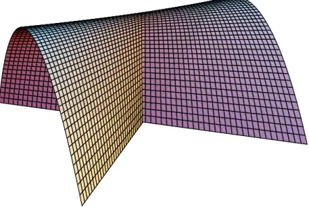
The first condition prevents situations like that found in the Whitney umbrella, which is illustrated in Figure 2.3. The “peak” of the umbrella forms a pinch point, which does not have a single, well-defined tangent plane. It is a well-known, but non-trivial fact that such a point cannot occur on the medial axis of a generic object.
The second condition ensures that M contains no degenerate pieces. For example, the medial axis of a circle in 2D is a single point, which is not part of a 1D manifold with boundary. Similarly, degenerate curves are produced by tubes in 3D, etc. Such degeneracies are not generic, in that a small perturbation of the shape makes them non-tubular. It may still be useful to create specialized shape models to handle them in order to avoid instabilities in how such a perturbation is chosen, as in (Damon, 2006). However, this dissertation focuses on the general case.
The third condition ensures that two pieces do not meet in a degenerate way. For example, if two medial sheets meet in 3D, they must do so along one-dimensional branch curve and not just at a zero-dimensional point.
The skeletal set, however, is just one part of the medial axis. We also need to define how the points on the medial axis relate to the boundary of the object. For the Blum medial axis, this is done in terms of the spokes, the vectors that lie normal to the boundary, but we start with a more general structure called the radial vector field, S. This vector field is defined over the set M and, like a number of other constructs we will use, ismultivalued. That is, it has multiple values at each point and not necessarily the same number of them at every point (cf. the arrows in Figure2.1(a)).
2Recall that in
Figure 2.3: The Whitney umbrella is an example of a stratified set that fails the first condition required of a skeletal set. It is given by the equation (x, y, z) = (uv, u,1−v2)
over the domain (u, v)∈[−1,1]2.
The purpose of the radial vector field is to give a mapping from a skeletal set to the object boundary. At regular points on the skeletal set, there are always two radial vectors, which correspond precisely to two points of tangency on the bitangent spheres. One corresponds to the “top” of the medial sheet, and the other corresponds to the “bottom”. However, smoothly extending the vector field to singular points may require one, three, or even more vector values at a single point.
We adopt a slightly non-standard definition ofsmooth at edge points to overcome a problem of parameterization. In order to have a closed boundary, at edge points the top vector field must continuously join with the bottom vector field on the corresponding smooth manifold component, Mα. However, like the function
√
x evaluated at x = 0, on a Blum medial axis the resulting vector fields are not differentiable on Mα,
because the slope lies perpendicular to the manifold. Damon uses an edge coordinate parameterization to overcome this limitation.
Definition 2.14 An edge coordinate parameterization at an edge closure point m0 ∈ ∂M lying on the boundary of the closure of a local neighboring component Mα
consists of an open neighborhood Nm0 ∈ Mα, an open neighborhood N˜0 ∈R
n−1
≥0 , and a
differentiable homeomorphism φ: ˜N0 →Nm0 such that both φ restricted to ( ˜N0∩R
n−1
and to ( ˜N0∩Rn−2) are diffeomorphisms.
The ( ˜N0∩Rn+−1) restriction corresponds to the parameterization of the local piece of
the neighboring manifold Mα, while ( ˜N0∩Rn−2) corresponds to the parameterization
along the edge curve. Then we say a scalar or vector field is smooth at an edge closure point if the composition with an edge parameterization is smooth. As a trivial example, √
x is smooth on x∈R≥0 under the edge parameterization φ(u) =u2. In general, any
smooth function on Mα is smooth under an edge parameterization, but as the
√ x example illustrates, the converse is not true.
Describing how smooth extensions work at non-edge singular points requires the introduction oflocal complementary components.
Definition 2.15 Given m0 ∈Msing and a closed ball B(m0)⊂ Rn, let Ci be the
con-nected components ofB(m0)\M. Again >0 is chosen to be sufficiently small so that
these are well defined (up to a homeomorphism). These are thelocal complementary
components of m0.
Definition 2.16 Givenm0 ∈Msing with local complementary componentsCi and local
neighboring components Mα, let ∂Ci , {Mα : Mα ∩Ci 6= ∅}. These are the local
neighboring components adjacent to Ci.
Definition 2.17 We say a vectorupoints into a local complementary component Ci
from a point m if there exists an >0 such that m+tu∈Ci for all 0< t < .
The idea will be to ensure that every local complementary component has exactly one radial vector pointing into it at each singular point m0. This, along with smoothness
constraints, ensures that the radial vectors do not poke through one of their neighboring strata, at least locally. Of course if the vector is too long, it may poke through a non-local piece of the medial axis, but in so doing it must of necessity cross other radial vectors. Later, we will show how to detect such crossings. But first, we give Damon’s complete definition of a radial vector field.
Definition 2.18 Given a skeletal set M ⊂ Rn, a radial vector field S on M is a
nowhere zero multivalued vector field satisfying the following conditions.
1. (Behavior at smooth points) LetN be a smooth unit normal vector field over each of the medial sheets inMreg. Then for each smooth pointm0 ∈Mreg, S has exactly
two values,S+ andS−, such thatS+· N(m
0)>0andS−· N(m0)<0. Moreover,
2. (Behavior at non-edge singular points) Let m0 ∈ Msing\∂M be a singular point
with local neighborhood component Mα. Then S+ and S− on Mα each extend
smoothly to a value ofS(m0). If there exists a neighborhoodNm0 such that Nm0∩
Mα ∩∂M = ∅, then that value S(m0) 6∈ Tm0Mα. Conversely, for each value
of S(m0), there is exactly one local complementary component Ci of M at m0
such that the value S(m0) locally points into Ci in the following sense. Let
Mα ∈ ∂Ci be a local neighboring component adjacent to Ci and let Nm0 be an
open neighborhood chosen sufficiently small so that Nm0 ∩Mα ⊂ Ci. Then for
all m ∈Nm0 ∩Mα, either N, −N, or both point into Ci. Let S
0 be a restriction
of S to the values where the corresponding normal direction points into Ci, along
with the value ofS(m0)under consideration. Then S(m0)smoothly extends to the
values ofS0 onMα. FurthermoreS0(m0)points intoCi and for allm ∈Nm0∩Mα,
S0(m) points into Ci.
3. (Tangency behavior at edge points) Letm0 ∈∂M be an edge point andMα ⊆Mreg
be the stratum whose edge it is, i.e., m0 ∈ Mα. Then S has exactly one value
S(m0) such that S(m0) ∈ Tm0Mα, and S(m0) points away from M. This value
extends smoothly into Mα (under some edge parameterization).
The radial vector field corresponds to the spokes linking the centers of the maximally inscribed balls to their points of tangency with the boundary in the Blum medial axis. In addition to the constraints in its definition, two local initial conditions must be satisfied:
1. (Local Separation Property) For each a non-edge point m0 6∈∂M, let Mα be the
local neighboring components, and letCibe the local complementary components
contained in the ball B(m0). Then for all m ∈ ∂Mα on the boundary of the
closures of the neighboring component with radial vector S(m) locally pointing into a given Ci, the set {m+tS(m) :t∈R≥0} ∩B(m0)⊂Ci.
2. (Local Edge Property) For each edge closure point m0 ∈ ∂M, there exists a
neighborhood Nm0 ⊂M and an >0 such that for each choice of smooth vector
fields S over W, the functionψ(m, t) =m+tS(m) is one-to-one on Nm0 ×[0, ].
that in a neighborhood around m0, for any fixed choice of one can find a spoke that
pierces the skeletal set before traveling a distance along it.
A skeletal set together with a radial vector field satisfying the local initial conditions is called askeletal structure. It is a far more general structure than a Blum medial axis, since the radial vectors are not explicitly required to be normal to the boundary, nor even the same length on each side. Several theorems presented later will apply to all skeletal structures, not just the Blum case.
2.3.3
The Blum Medial Axis as a Skeletal Structure
A skeletal structure, as defined, does not have a radius associated with each point, but we can partition the radial vector field into two parts: S = rU, where r = kSk is a positive function (obeying smoothness constraints similar to those on S), and U is a unit radial vector field. On the smooth parts of M, we will use U± to denote the two unit radial vectors on either side. In general, r is multivalued, but for a Blum medial axis, all of the values at a single point must be equal, e.g., all the spoke values must be the same length. Also, r is allowed to be zero in Definition 2.4, but in a skeletal structure it must always be positive. The only places that the radius would go to zero are sharp, non-smooth corners or creases. These are not generic, as they make the boundary undifferentiable at those points, so they are intentionally disallowed.
On the Blum medial axis the radial vectors correspond to the points where the maximally inscribed balls are tangent to the boundary of the object. This gives rise to relation between r and U described by the compatibility one-form3. It is defined as ηU ,ωU +dr, where ωU(v), U ·v is the one-form dual of U, and dr is the one-form
defined by the directional derivative of r. Like U, ηU is multivalued. Lemma 6.1 of
(Damon, 2003) states that if ηU ≡ 0 at a point m0, then U(m0) is orthogonal to the
boundary at m0+rU(m0). HereηU ≡0 means that for all v ∈Tm0M, ηU(v) = 0. The
tangent space at singular points is chosen to correspond to the limiting tangent space of a local neighboring component for which U(m0) is a smooth extension. There can
be more than one such local neighboring component for a particular value of U(m0)
and hence more than one tangent space and more than one value of ηU. ηU ≡0 holds
only if ηU(v) = 0 holds forall choices of ηU and limiting tangent spaces at m0. Damon
terms this thepartial Blum condition. By itself it is sufficient to describe the geometry of the boundary of an object, even whenrordr has multiple distinct values at a point.
3Aone-formis a linear functionω1mapping a vector to a scalar,ω1(v) :
Rn→R, e.g., it has “one
We can use the partial Blum condition to derive an explicit formula forU in terms of r on the smooth points Mreg. The immediate implication is that the component of
U in the tangent plane is−∇r, where ∇r ∈Tm0M is the Riemannian gradient
4. This vector lies in the tangent space Tm0M and is independent of the parameterization of
r and M. Since U(m0) is a unit vector, this leaves only two possible choices for the
component normal to the tangent plane, one for each side:
U± =−∇r±p1− k∇rk2· N (2.3)
This definition can then be smoothly extended to points in Msing. It is independent
of dimension and generalizes earlier formulas given by (Blum and Nagle, 1978) for two dimensions, and (Nackman, 1982) and (Giblin and Kimia, 2004) for three.
On the Blum medial axis, where r and thus∇r are single-valued, the vector (U+−
U−) points in the normal direction N of M, and the bisector 12(U++U−) lies in the
tangent spaceTm0M. Furthermore, at edge points, by Definition2.18(3) one must have
U(m0)∈ Tm0M, implying the normal component vanishes. Hence, at these points we
have
k∇rk= 1 . (2.4)
In the complementary component Ci of a non-edge singular point m0 ∈Msing, each
of the local neighboring componentsMα ∈∂Ci must contribute a spokeS(m0) pointing
intoCi by smooth extension, and all of theseS(m0) values must be equal. Using (2.3),
we can write this as a constraint on ∇r in each of the local neighboring components. For example, on branch curves in 3D, given three local componentsMk oriented so that
S(k)−(m0) = S(k⊕1)+(m0), the restriction becomes (Yushkevich et al., 2003)
∇r(k⊕2)− ∇r(k⊕1) =N(k)·q1− k∇r(k)k2 , (2.5)
where ⊕ denotes addition modulo 3. At fin creation points, k∇r(k)k goes to 1 for one
of the sheets, causing the angle between the other two to go to π, and the constraint in (2.5) to disappear.
Enforcing the two conditions in (2.4) and (2.5) will become the primary focus of Chapter 3.
2.3.4
Geometry of the Boundary
Given a skeletal structure (M, S), we have only guaranteed that the radial vectors S do not cross in a small neighborhood of the space around M. In order to ensure that the boundary associated with a skeletal structure is smooth, we must ensure that no such crossings occur anywhere along the entire length of the spokes. These can be classified into local intersections and non-local intersections (Hoffman and Vermeer, 1994). Non-local intersections are caused when two spokes separated by a non-trivial distance intersect, e.g., when one end of an object wraps around and abuts another. These are difficult to describe mathematically but for most objects are relatively easy to avoid during the modeling process by using geometric priors. Local intersections, on the other hand, occur when two spokes that originate from within an arbitrarily small neighborhood of each other on M cross somewhere along their length (not necessarily close to M), causing the boundary to fold over on itself, as illustrated in Figure 2.4. These can be detected by using aradial shape operator,Srad, on non-edge points and a
similaredge shape operator, SE, on edge points.
The radial shape operator is not an ordinary shape operator in the differential geometric sense. The traditional shape operator measures how the unit normal N changes for an infinitesimal step along the surface of a manifold; it is a linear map that can be expressed as a self-adjoint matrix for any choice of orthonormal basis. Its eigenvalues are called the principal radial curvatures.
The radial and edge shape operators, in contrast, give the components of the change in the radial vectorsU for such an infinitesimal step onM and ∂M, respectively. They are linear operators but are not in general self-adjoint. The eigenvalues of Srad are
termed the principal radial curvatures κr i, and the generalized eigenvalues of SE the
principal edge curvatures κE i. Their definition now proceeds.
Definition 2.19 Given a non-edge point m0 ∈M \∂M of M and a choice of smooth
values of S on a stratum Mα or the closure of a local neighboring component Mα
containing m0 with tangent space Tm0M, the radial shape operator Srad :Tm0M →
Tm0M is defined as
Srad(v) = −projU(
∂U
∂v) . (2.6)
Here, projU denotes projection ontoTm0M alongU, which is in general not orthogonal
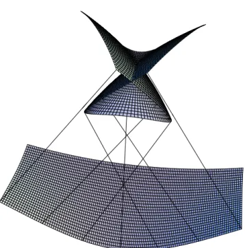
Figure 2.4: An example of overfolding, causing a swallowtail singularity in the bound-ary. The top surface is one half of the boundary, the bottom is the medial sheet, and the lines connecting them denote the spoke field. The radial shape operator detects this overfolding everywhere in the bottom segment of the swallowtail, where the spokes exhibitretrograde motion: a step forward along the medial axis causes a step backwards along the boundary.
will have two values, one for each value of U, and at non-edge singular points m0 ∈
Msing\∂M each local neighboring component Mα will contribute two values via the
smooth extension ofU onto m0.
For a given (not necessarily orthonormal) basis of Tm0M, v = {v1, . . . , vn−1}, Srad
can be represented by an (n−1)×(n−1) matrixSv. The precise details of calculatingSv
for a parameterized surface in 3D are given in AppendixA. BecauseU is not necessarily normal and the projection is not orthogonal, Sv will not in general be self-adjoint, so
its eigenvalues need not be real. Nevertheless, these eigenvalues, which are independent of the choice of basis, form what are termed the principal radial curvaturesκr i. If the
κi, given by
κi =
κr i
1−rκr i
, κr i =
κi
1 +rκi
. (2.7)
This holds so long as 1r is not an eigenvalue ofSrad, which corresponds to a non-smooth
singularity of the boundary.
We can also define radial analogues of the mean curvature and Gaussian curvature, namely the mean radial curvature Hrad and the Gaussian radial curvature Krad. They
are defined exactly like their classical counterparts, except using Srad instead of the
traditional shape operator:
Hrad ,
1
2trace(Srad) , Krad ,det (Srad) . (2.8) Again, these numbers are the same irrespective of the choice of basis.
Every operation in this dissertation involvingSrad in three dimensions can be defined
in terms of these two numbers. The principal radial curvatures κr i can be recovered
via
κr i =Hrad±
p
Hrad2−Krad . (2.9)
And the usual relations hold:
Hrad =
κr1+κr2
2 , Krad =κr1κr2 . (2.10)
We now turn to the edge shape operator, SE.
Definition 2.20 Given an edge pointm0 ∈∂M lying in the boundary of the closure of
a local neighboring component Mα with tangent space Tm0M, a choice of smooth values
of U on Mα, and a unit normal vector field N on Mα, the edge shape operator
SE :Tm0M →Tm0∂M ⊕ hN i is defined as
SE(v) = −proj0U(
∂U
∂v) . (2.11)
Now proj0U denotes projection onto Tm0∂M ⊕ hN i along U, which again is not in
a (not necessarily orthonormal) basis ˜v={v1, . . . , vn−2} of Tm0∂M and adds a vector
vn−1 that points in the U(m0) direction under the edge coordinate parameterization to
form a basis v = {v1, . . . , vn−1} of Tm0M. The basis of the destination space is then
taken as ˜v N
. Then, lettingIn−2,1 denote the (n−1)×(n−1) diagonal matrix with a
one in the first (n−2) diagonal elements and zeros everywhere else, the principal edge curvaturesκE i are defined as the generalized eigenvalues5 of (SEv,In−2,1).
Suppose we are given a skeletal structure (M, S) satisfying the following conditions: 1. (Radial Curvature Condition) For all points m0 ∈ M \∂M, r < κ1r i for all real,
positive principal radial curvatures κr i.
2. (Edge Curvature Condition) For all pointsm0 ∈∂M,r < κ1
E i for all real, positive
principal edge curvaturesκE i.
3. (Compatibility Condition) For all singular points m0 ∈Msing,ηU ≡0.
Theorem 2.5 of (Damon, 2003) states that if the associated boundary B has no non-local intersections, it is an embedded manifold that is smooth at all points except those corresponding to points in Msing. At points corresponding to the singular points Msing,
it has G1 continuity, i.e., it has a well-defined tangent plane.
The compatibility condition is just the partial Blum condition restricted to singular points. If we add the partial Blum condition everywhere and restrict r to be single-valued, we obtain the following lemma.
Lemma 2.21 Suppose(M, S) is a skeletal structure satisfying the radial and edge cur-vature conditions and the partial Blum condition and further suppose that the associated radius function r is single-valued. Then if the associated boundary B has no non-local intersections, it is an embedded manifold that is smooth at all points except those cor-responding to points in Msing, where it has G1 continuity. Furthermore, if every ball
defined by M is contained in the interior of the object, M is the Blum medial axis of B.
This is the main result of this section. Given a generative model for a medial axis, it tells us what conditions need to be checked to ensure the associated boundary is legal, in the sense that it could be the boundary of a real, physical object. We start with a single-valued r and derive U and hence S from (2.3), ensuring that the partial
5The generalized eigenvalues of a pair of matrices (A,B) are the values λ such that A−λB is
Blum condition holds by construction. The most difficult part is then ensuring that the behavior of U at singular points is sufficient to make it a valid radial vector field, which is the subject of Chapter 3. Then all that remains is to verify the radial and edge curvature conditions, and check for non-local intersections. The first is done as the model evolves to fit a particular shape in Chapter 4, and the assumption that our shapes are sufficiently well-behaved makes checking the second unnecessary.
Because the edge shape operator requires an edge coordinate parameterization, it is more difficult to deal with than the radial shape operator. However, since almost all of the points on the medial axis are smooth points, in general it is substantially less useful. The edge curvature condition is technically required for a smooth boundary, but so long as a sufficient margin of safety is kept in the radial curvature conditions, it cannot be violated. Therefore the remainder of this work will not devote a great deal of effort to its analysis.
2.3.5
Integrals Over Skeletal Structures
The ability to compute integrals over an object Ω and its boundary Busing medial co-ordinates is an invaluable tool. Trivial examples include computing the volume, center of mass, or second order moment of an object defined by its medial axis. These are later used to align two or more objects. More complex examples include the geometry to image match function used to fit a model to a given shape, as in Chapter4. Because the model is defined via its medial axis, the medial coordinate system provides a natu-ral way to parameterize these integnatu-rals. Damon shows how to define a medial measure dM that makes M into a measure space and consequently how to write formulas for these integrals (Damon, 2005a).
One conceptual difficulty that arises is that integration must take place on “both sides” of M. To do this, Damon introduces the “double” ofM, denoted ˜M.
Definition 2.22 Thedoubleof a skeletal structure(M, S)is the setM˜ ={(m0, S0)∈
Rn×Rn:m0 ∈M and S0 is a value of S at m0}.
The vectorsS0 serve to label each “side” of the smooth strata in Mreg. As the notation
indicates, points of ˜M should be thought of as a point on the medial axis together with a direction, and not as the associated point on the boundary, m0 +S0.
The definition of a topology on ˜M proceeds from a system of neighborhoods. Definition 2.23 Let (m0, S0) ∈ M˜ be a point in the double of M, W0 be an open
m0 into whichS0 points. Then the abstract neighborhood of (m0, S0)is given by the
set W ={(m, S0)∈M˜ :m ∈W0∩∂C
i and S0 points into Ci}.
Then ˜M can be decomposed into a Whitney stratified set so that the canonical projec-tion π : ˜M → M given by π(m0, S0) = m0 is continuous and smooth with respect to
this neighborhood system.
The definition of the skeletal integral of a multivalued function f onM now follows from assuming thatfhas one value corresponding to each value ofSat a pointm0 ∈M,
so that f lifts to a well-defined function ˜f : ˜M → R given by ˜f = f ◦ π. Then Proposition 2.2 of (Damon, 2005a) states that there is a unique regular positive Borel measuredM on ˜M such that the integral of f on M is given by
Z
˜
M
˜
f dM . (2.12)
The measure dM is called the medial measure, and it is given by dM = ρ dA, where dAis the ordinary (n−1)-dimensional differential unit of area onM, and ρ=±U±· N
on points in Mreg. Values on Msing are defined by smooth extension from the local
neighboring components. At edge points ∂M it is exactly zero, and the total measure of the whole set Msing is also zero, meaning that so long as f is bounded on Msing,
the singular points may be ignored for purposes of integration. For a generic skeletal structure, ρ is multivalued, but on the Blum medial axis it is actually single-valued overMreg, thanks to the symmetry of U±.
The factor ρcorrects for the failure of S to be orthogonal toM. Thus, areas where S is nearly tangent to M are “small” with respect to this measure. For example, adding a small bump to the boundary of an object can create a spurious branch on the medial axis, but all of the spokes will be nearly tangent to this branch, making their contribution to any integral small.
This integral has the usual linearity and positivity properties, e.g., RM˜ f˜+ ˜g dM =
R
˜
Mf dM˜ +
R
˜
Mg dM˜ and if ˜f ≥ 0,
R
˜
Mf dM˜ ≥ 0. We say that f is measurable and
integrable on M if ˜f is measurable and integrable on ˜M. Damon calls this a skeletal integral and, in the special case where (M, S) satisfies the partial Blum condition, a medial integral.