Probing protein structural dynamics using simplified models

Probing Protein Structural Dynamics using

Simplified Models

Yiwen Chen

A dissertation submitted to the faculty of the University of North

Carolina at Chapel Hill in partial fulfillment of the requirements for

the degree of Doctor of Philosophy in the Department of Physics and

Astronomy

Chapel Hill

2007

Approved by:

Dr. Richard Superfine

Dr. Nikolay V. Dokholyan

Dr. Sharon L. Campbell

Dr. Sean Washburn

©2007

Yiwen Chen

ABSTRACT

YIWEN CHEN: Probing Protein Structural Dynamics using

Simplified Models

(Under the direction of Dr. Nikolay V. Dokholyan)

Structure and dynamics play crucial roles in many aspects of protein function. The detailed characterization of structure and dynamics of a protein is therefore critical for elucidation of its function. Despite the rapid advances in experimental methods, we are still much limited in our ability to characterize the structure and dynamics of a protein due to the resolution capability at length and time scales of the current methods. As complimentary approaches to the experimental methods, coarse-grained simulations based on simplified models offer unparallel opportunities for studying structure and dynamics that are hardly subject to direct experimental characterization.

fidelity of protein structure reconstruction using inter-residue proximity constraints and rational strategies for constraint selection for protein structure determination.

Dedicated to my parents,

ACKNOWLEDGEMENTS

TABLE OF CONTENTS

LIST OF TABLES...

ix

LIST OF FIGURES ...

x

I. INTRODUCTION

General background ... 1 Experimental tools for studying protein structure and dynamics ... 7 Theoretical/computational methods... 16

II. COMBINING HYDROGEN EXCHANGE DATA AND

COARSE-GRAINED SIMULATION TO CHARACTERIZE FOLDING

INTERMEDIATE OF FAT DOMAIN

Introduction... 23 Materials and methods ... 25 Results and discussion ... 29

III. CHARACTERIZING THE LARGE-SCALE STRUCTURAL DYNAMICS

OF VINCULIN RELATED TO ITS ACTIVATION

Introduction... 42 Materials and methods ... 44 Results and discussion ... 48

IV. DETERMINING PROTEIN STRUCTURE USING INTER-RESIDUE

PROXIMITY CONSTRAINTS

Materials and Methods... 65

Results and Discussion Conclusions... 69

Conclusions... 80

LIST OF TABLES

Table

LIST OF FIGURES

Figure

1.1

The reaction scheme of hydrogen exchange ... 15

1.2

An illustration of the principle of hydrogen exchange experiments... 16

1.3

The two principal components of a sample two-dimensional data set ... 17

1.4

A flowchart illustration of Monte Carlo Metroplis algorithm ... 19

1.5

Difference between traditional molecular dynamics and discrete molecular dynamics simulation... 20

1.6

A sample graph and two sub-graphs ... 22

2.1

Energy map for the FAT domain ... 30

2.2

Correlation between experimental and calculated protection factors ... 31

2.3

The folding trajectory for the scaled DMD simulations ... 33

2.4

The probability distribution at three simulation temperatures ... 34

2.5

Frequency map for the intermediate ensemble ... 35

2.6

Comparison of the FAT domain intermediate from DMD simulations with the domain-swapped dimer... 37

3.1

The native structure of full-length vinculin ... 50

3.2

The thermal melting curves of inter-domain and intra-domain interactions ... 52

3.3

A cartoon representation of the sequential unfolding events in the kinetic simulation 54

3.4

A sample trajectory from kinetic unfolding simulations ... 55

4.1

The average and the standard deviation of RMSD of the structural ensembles for nine small protein domains... 72

4.2

The average and the standard deviation of RMSD of the structural ensembles for two large protein domains... 73

4.3

The average and standard deviation of RMSD of the structural ensembles for

ABBREVIATIONS

ECM Extracellular matrix FAK Focal adhesion kinase

PTM Posttranslational modification NMR Nuclear magnetic resonance

HSQC Heteronuclear single quantum correlation NOE Nuclear Overhauser Effect

NOESY Nuclear Overhauser Effect Spectroscopy

RF Radio frequency

ESI Electrospray ionization

MALDI Matrix-assisted laser desorption/ionization MS/MS Tandem mass spectrometry

HX Hydrogen exchange

PCA Principal component analysis DMD Discrete molecular dynamics FAT domain Focal adhesion targeting domain Vt Vinculin tail domain

VASP Vasodilator-stimulated phosphoprotein Arp2/3 Actin-related protein complex

RMSD Root-mean-square-deviation

CITATIONS TO PUBLISHED WORKS

Chapter 2, 3, and 4 were reproduced with modifications based on three published works. The permissions for the reproduction of figures and texts in the dissertation were granted by the publishers.

Chapter 2 was published in Structure12, Dixon, R.D., Chen, Y., Ding, F., Khare, S.D., Prutzman, K.C., Schaller, M.D., Campbell, S.L., and Dokholyan, N.V. (2004), New insights into FAK signaling and localization based on detection of a FAT domain folding

intermediate, 2161-2171. Copyright © 2004 Elsevier Ltd.

Chapter 3 was published in Journal of Biological Chemistry 281, Chen, Y. and Dokholyan, N.V. (2006), Insights into allosteric control of vinculin function from its large-scale

conformational dynamics, 29148-29154. Copyright © 2006 the American Society for Biochemistry and Molecular Biology

Chapter 4 was reproduced in part with permission from Journal of Physical Chemistry B111, Chen, Y., Ding, F., and Dokholyan, N.V. (2007), Fidelity of the protein structure

CHAPTER 1

INTRODUCTION

General background

Protein

Proteins are linear biopolymers that are composed of 20 different amino acids(Branden and Tooze, 1999). All amino acids share a common chemical structure including a central carbon (Cα) atom to which an amino group (NH2), a carboxyl (C’OOH) and a side chain are attached.

Primary, secondary, tertiary and quaternary structure

Most proteins fold into a unique three-dimensional structure which is known as its native structure/state(Branden and Tooze, 1999). A three-dimensional structural unit that can fold independently within a protein is called a domain. A protein is known as single-domain if it has only one domain, otherwise it is called a multi-domain protein. A series of terminologies are used to describe different hierarchies of protein structure. Primary structure refers to the ordered sequence of amino acids (from N-terminus to C-terminus) that compose the protein. Secondary structure refers to the regularly repeating local structures that are stabilized by hydrogen bonds. The most common examples of secondary structure are the alpha helix and beta sheet. The spatial arrangement of the secondary structures i.e. overall topology of a single protein is known as its tertiary structure. The overall three-dimensional structure of a protein complex that results from the assembly of more than one protein is known as quaternary structure. Each protein in the protein complex is usually called protein subunits. Proteins can be roughly classified as globular proteins, fibrous proteins, and membrane proteins. Most of the globular proteins are soluble; while many membrane proteins are insoluble in water and therefore more difficult to study. Fibrous proteins often play structural roles in cellular functions.

Extracellular matrix

Extracellular matrix (ECM) is the part of a tissue that is not part of any cell in the tissue(Lodish et al., 2004). The main components of the ECM are proteoglycans , glycoproteins, and hyaluronic acid. It also contains proteins including fibrin, elastin,

fibronectins, lamins, and nidogens, and other substances such as minerals or fluids. Moreover, it acts as a reservoir for a wide variety of growth factors, the release of which can cause the rapid alteration of physiological states of cells. In overall, it serves as a micro-enviroment for the cells by providing support and anchorage for cells as well as regulating cell signaling. It is essential to maintaining the physiological structure and function of a tissue.

Focal adhesion

Focal adhesions are integrin-rich cell adhesion sitesthat make close contact to the

ECM(Lodish et al., 2004). This physical interaction confers cells the ability to communicate with outside environment, which is essential for cell adhesion, migration, proliferation and death. At molecular level, focal adhesions are comprised of large molecular complexes forming around an integrin heterodimer. Integrin binds to ECM proteins through its

extracellular domain. The cytoplasmic domain of integrin binds to the cytoskeleton through adapter proteins such as α-actinin, filamin, talin and vinculin. Many cell signalling proteins, such as focal adhesion kinase (FAK), associate with this integrin-adapter

protein-cytoskeleton complex, which is the molecular basis for a focal adhesion to connect the actin cytoskeletons to the cytoplasmic side of the membrane, and mediates intracellular

stimuli, which inform the cell about the micro-environment. In non-moving cells, focal adhesions are relatively stable, whereas in moving cells they constantly assemble and disassemble as the new contacts form at the leading edge, and dissemble at the trailing edge of the cell when old contacts are broken.

Cell-cell adhesion

The adhesion of one cell to another is critical to the formation and maintenance of tissues in multi-cellular organism(Lodish et al., 2004). At cell-cell contact sites, the extracellular domains of transmembrane adhesion molecules interact with molecules on the surface of adjacent cells, and the cytoplasmic domains are associated with the cytoskeleton through various adaptor proteins. Connecting the cytoskeleton to adjacent cells confers mechanical strength to tissues and provides physical basis for the cytoskeletal movements that mediate changes of cell morphologies during development. Cell-cell adhesion is tightly controlled during processes that require detachment and reattachment between cells, such as cell

are connected to the intermediate filaments. In all of these junctions, the presence of adaptor proteins in the adhesion molecule–cytoskeletal linkage provides targets for regulatory signals that control the strength and assembly of cell contact sites. In general, cell adhesion proteins are classified based on the structure of the adhesion proteins and their corresponding ligands. Adhesion between two molecules of the same adhesion protein is called "homophilic" binding, and adhesion between an adhesion protein and a different type of protein is called "heterophilic" binding(Lodish et al., 2004).

Cell migration

Cell migration is a central process in the physiology of multi-cellular organisms. It plays essential roles in the processes such as embryonic development, wound healing and immune responses. The aberrant migration of cells is often related to serious human diseases

including mental retardation, vascular disease, rheumatoid arthritis, and cancer. Therefore the understanding the basic mechanisms of cell migration holds the promise of effective

therapies for treating diseases(Ridley et al., 2003).

of which is often correlated with the motility of a cell(Friedl and Wolf, 2003; Knight et al., 2000; Ridley et al., 2003).

Although, this general picture is shared by many cell types, the details may differ significantly. For example, this cyclic process is pronounced in slow-moving cells such as fibroblast, but not as obvious as in fast-moving cells such as neutrophils. In addition, the way how cell migrates highly depend on its environment. For instance, somitic cells migrating in vivo exhibit large single protrusions and highly directed migration, which is distinct from the multiple small protrusions they show on planar substrates; cancer cells are able to modify their migratory behavior and morphology in response to environmental changes(Knight et al., 2000; Ridley et al., 2003).

As a highly coordinated process, cell migration involves a complex network of

interaction between different proteins. FAK and vinculin, which are two major subjects of study in this dissertation, play significant roles in this process.

Phosphorylation

After protein translation, the posttranslational modification (PTM) of amino acids can alter protein function by attaching to it other biochemical functional groups such as acetate, phosphate, various lipids and carbohydrates, which changes the chemical nature of an amino acid. Phosphorylation is the addition of a phosphate (PO4) group to a protein and an

proteins are activated or deactivated by phosphorylation and dephosphorylation.

Phosphorylation is catalyzed by various specific protein kinases, whereas dephosphorylation of a protein is catalyzed by the machineries, called phosphatases.

Experimental methods for studying protein structure and dynamics

Nuclear magnetic resonance spectroscopy

Protons and neutrons have a spin angular momentum with a value of +1/2 or -1/2. Protons or neutrons in the atomic nucleus can pair with other protons or neutrons with anti-parallel spin angular momentums. A nucleus with all protons and neutrons that are in pair has a net spin angular momentum of zero, but a nucleus with unpaired protons or neutrons will have a non-zero overall spin. When the spin angular momentum of a nucleus is non-zero, it has an associated magnetic moment μ, which is utilized for manipulation in nuclear magnetic resonance

(

NMR) experiments(Cavanagh et al., 1996). The nuclei that have odd numbers of nucleons (protons and neutrons) have a non-zero intrinsic magnetic moment. The most commonly used nuclei in NMR experiments are 1H, 13C and 15N. NMR studies the nuclear spin dynamics of a magnetic nucleus by aligning its nuclear spin with a large external magnetic field and perturbing this alignment using an electromagnetic pulse field. The response of nuclei to the perturbation using pulse field is what is monitored in NMR

Nuclear spin angular momentum is a vector quantity. The Z component (the component along the direction of external magnetic field) of the nuclear spin angular momentum, Iz can

take values ranging from +I to –I in integer steps where I is the magnitude of nuclear spin angular momentum(Cavanagh et al., 1996). For a given nucleus with spin angular

momentum I, there are in total (2I+1) angular momentum states along Z-axis. Therefore the Z

component of spin angular momentum Iz, is quantized as follows:

(

)

2

Z

h

I

m

I

m I

π

=

− ≤ ≤

where h is Planck's constant and π is a mathematical constant, i.e. the ratio of a circle's circumference to its diameter in Euclidean geometry . The magnetic moment of this nucleus is related to its spin angular momentum with a proportionality constant γ, which is called the gyro-magnetic ratio:

Z Z

γ

I

μ

=

For a nucleus that has a spin of one-half (I=1/2), the nucleus has two possible Z

component of the spin angular momentum Iz: +1/2 or -1/2 (up or down state). The energies of

these two spin states are degenerate in the absence of external magnetic field. When a nucleus is subject to a magnetic field, the two magnetic momentum states no longer have equal energy since the energy of a magnetic moment μ in a magnetic field B0 is the negative

scalar product of the two vectors:

0

B

E

=

−

μ

_Z ,

where μz is the Z component of the nuclear magnetic moment and magnetic field is along

0

1 1

(

,

2

2

mh B

E

m

)

2

γ

π

= −

= −

_,

The energy gap between the two spin states is then (hγBB0)/2π. A resonance can occur between

these two states when a radiofrequency (RF) is applied with the same energy as the energy difference ΔE between the two spin states. The energy of a RF photon is E =hν, where ν is its frequency.

_π

γ

2

0

B

h

E

=

Δ

Thus, the frequency of electromagnetic radiation required to produce resonance of a specific type nucleus in a field BB0 is:

0 0

2

B

v

γ

π

=

This resonance gives rise to the nuclear magnetic resonance spectrum. Since other nuclei, especially spin-active nuclei, and local electron are able to shield each probed nucleus differently from the main external field BB0, the strength of the effective magnetic field BeffectiveB

at the nucleus is different from the applied magnetic field BB0. Therefore the frequency

necessary to achieve resonance becomes 2

eff B

γ

π and is different from the expected value of

0

2

B

γ

frequency

0 eff ref

v v

v

−

is called chemical shift. For nuclei in different chemical environments,

the chemical shifts are usually different(Cavanagh et al., 1996). The chemical shit differences between nuclei give rise to distinct peak frequencies in a nuclear magnetic resonance

spectrum, which forms the basis for NMR spectroscopy to be a direct probe of chemical environment of a nucleus. The chemical environment of a nucleus in a protein often changes when a protein undergoes transitions between several conformations, which are induced by the binding of a substrate to the active site of an enzyme, or a protein ligand to the

protein(Cavanagh et al., 1996).

Heteronuclear Single Quantum Correlation

A heteronuclear single quantum correlation (HSQC) is an experiment frequently used in protein NMR spectroscopy(Cavanagh et al., 1996). The HSQC spectrum has two axes, a proton axis and a hetero-nuclei axis. A hetero-nucleus is another nucleus other than protons, which is most often 13C or 15N. The peaks in the HSQC spectrum usually correspond to different protons attached to hetero-nuclei.

essential for interpretation of more advanced NMR experiments and an important procedure for protein structure determination.

The HSQC experiment is also useful for detecting protein-protein, protein-ligand or protein-drug interactions. By comparing the HSQC of the free state of a protein with its bound-state, it is possible to find out the binding interface where the chemical shifts of the peaks are most likely to change.

Nuclear Overhauser Effect Spectroscopy

Overhauser Effect generally refers to the transfer of spin polarization from one spin

population to another. Overhauser effect can occur between electrons or atomic nuclei. The spin polarization transfer is commonly observed and used amongst atomic nuclei and named Nuclear Overhauser Effect (NOE)(Cavanagh et al., 1996). A commonly-applied technique in structural biology that is based on NOE is Nuclear Overhauser Effect Spectroscopy

(NOESY). NOESY spectra provide distance information about protons that are within 5 Angstroms. The NOESY spectrum obtained in the experiment has two proton axes. The presence of a NOE peak between two protons indicates that the corresponding protons are within 5 Angstroms through space and the intensity of the peak is proportional to 1₆

Mass spectrometry

Mass spectrometry is a powerful tool that is used to analyze and identify the composition in a mixture based on the difference of the mass-to-charge ratio of constituent components. The basic idea of mass spectrometry is that by applying electric and magnetic fields to the ionized molecules, different components in the samples have different modes of motions in space or time, due to their difference in mass-to-charge ratio, so that one can separate and detect them based upon this spatial or temporal difference. Due to its incomparable power, it is becoming an indispensable tool in identifying specific proteins and the post-translational modifications of the proteins in a complex biological sample. There are three major components that constitute a mass spectrometry: ion source, mass analyzer, and detector.

The ion source ionizes the material of interest and the generated ions are then passed to the mass analyzer by applying magnetic or electric fields. Ionization techniques have been key determinants for the type of samples (liquid or solid samples) to be analyzed by mass spectrometry. There are two major techniques that are used with liquid and solid biological samples, respectively: electrospray ionization (ESI) and matrix-assisted laser

desorption/ionization (MALDI)(Hoffmann and Stroobant, 2001).

ESI is a technique that generates ionized liquid droplets through electrostatic charging. In ESI, liquid sample is first passed through a nozzle. The droplets are then generated by

used in liquid chromatography-mass spectrometry because it provides a natural liquid-gas interface that is capable of coupling liquid chomatography with mass

spectrometry(Hoffmann and Stroobant, 2001).

In contrast, in MALDI, the ionization is triggered by a laser beam shedding on a solid matrix that is used to protect proteins from being damaged by direct shedding of laser beam(Hoffmann and Stroobant, 2001). In MALDI, a chemical solvent is mixed with the protein molecule of interest and then spotted onto a MALDI plate.The solvent molecules vaporize, leaving the proteins and the matrix co-crystallized in a MALDI spot. When a laser is shed at the crystals in the MALDI spot, the spot absorbs the laser energy and the matrix becomes ionized. The matrix transfers part of its charge to the protein molecule, thus ionizing them while still protecting them from the possible destruction of the laser.

The mass analyzer is used to separate molecules by applying electric and magnetic fields to change the motion modes of ions in space and time(Hoffmann and Stroobant, 2001). Mass analyzers separate the ions according to their mass-to-charge ratio based upon the dynamics of charged particles in electric and magnetic fields in vacuum, which is described by the following equation:

m_q a E v B G G G G

× + =

)

( _,

This differential equation describes the classic equation of motion of charged particles. It completely determines the particle's motion in space and time when the particle's initial conditions are defined, and therefore forms the physical basis of every mass analyzer. It follows from this equation that two particles with the same physical quantity m/q behave exactly the same. Thus all mass spectrometry measure m/q. Different mass analyzers use either static or dynamic fields, or magnetic or electric fields, but all operate based on the same equation. The most commonly-used analyzers are time-of-flight, quadrupole and quadrupole ion trap. Many mass spectrometry use two or more mass analyzers for tandem mass spectrometry (MS/MS)(Hoffmann and Stroobant, 2001).

The last but not the least component of the mass spectrometry is the detector. When an ion passes by or hits a surface, the charge induced or current produced is recorded by the detector(Hoffmann and Stroobant, 2001). The recorded signal then gives rise to a mass spectrum comprised of a record of ions as a function of m/q.

Hydrogen Exchange (HX)

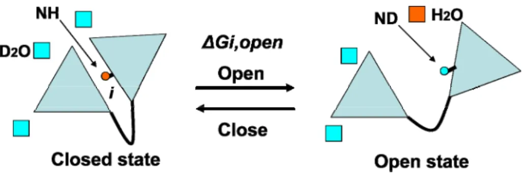
Hydrogen exchange (HX) is a chemical reaction in which a covalently bonded proton in a protein is replaced by a deuteron from solvent. Usually the examined protons are the amide proton in the backbone(Englander et al., 1996; Englander et al., 1997). HX of amide proton can be monitored by either NMR spectroscopy or mass spectrometry. For a typical NMR HX experiment, a protein of interest is put into deuterium water D2O. HSQC spectra are then

exchanges. The exchange constant is then obtained by fitting an exponential function to the data. When an amide proton is buried in a protein or forms intermolecular hydrogen bonds, it is protected against exchange with deuterons from solvent(Krishna et al., 2004). A protein has to undergo a conformational change from a well-folded state (C) in which the given amide proton is protected from exchange to an open state (O) where the same amide proton is competent for exchange (Figure 1.2)(Englander et al., 1996). Such a reaction scheme is shown in Figure 1.1., where kopenis the first-order rate constant for the transition from the

folded protein to the open state and kclose is the rate constant of the reverse transition. krc is the

intrinsic rate constant for exchange of amide proton with deuterium atom. Under EX2 condition where kclose>> krc, the effective exchange rate constant is rc op rc

close open

ex k K k k

k

k = = (Clarke

and Fersht, 1996; Englander, 2000).

FIGURE 1.1. The reaction scheme of hydrogen exchange

Therefore by dividing the effective exchange rate constant kex with tabulated intrinsic rate

constant krc for exchange of amide proton, the equilibrium constant of opening reaction Kop

Given its capability in probing the structural information of weakly-populated states of a protein that are difficult to study by other experimental methods, HX experiment is an

important tool for elucidating protein folding pathways, protein dynamics and protein-protein interactions(Clarke and Fersht, 1996; Englander, 2000; Wand and Englander, 1996).

FIGURE 1.2. An illustration of the principle of hydrogen exchange experiments. A protein has

to undergo a conformational change from a closed state in which the given amide proton is

protected, to an open state where the same amide proton is competent for exchange. Under EX2

limit, the free energy cost of opening reaction of a given amide proton can be estimated from

HX experiment.

Theoretical/computational methods

Principle Component Analysis

Principal components analysis (PCA) is a statistical technique for simplifying the representation of a data set, by reducing multidimensional data sets to lower

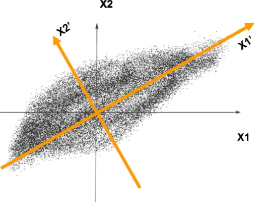
data lies on the first coordinate axis in the new coordinates, the second greatest variance on the second coordinate axis, and so on. The coordinate axes along which the greater variances of the data lie are called principal components. By keeping lower-order principal components and ignoring higher-order ones, PCA are used to reduce the dimensionality of the data set while retaining those features of the data set that contribute most to its variance. For example, in a two-dimensional data set that is shown in Figure 1.3, the two principle component axes are shown in orange. It is clear from figure that the variations of this data set along the first principal component accounts for most of variations in this dataset.

FIGURE 1.3. The two principal components of a sample two-dimensional data set are shown in

Monte Carlo Metroplis algorithm

In this algorithm(Binder, 1995; Liu, 2001), a stochastic search is performed in the

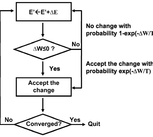
configuration space of interest through multiple iterations. The stochastic search is designed so that the points visited in the configuration space are distributed according to certain probability distribution that is of interest. At each point on the path of stochastic search, a random trial move from the current position in configuration space is generated. This trial move is then either rejected or accepted according to certain probabilistic rule. If the move is accepted then the search proceeds starting from the new position in configuration space; otherwise there is no move in configuration space. Another trial move is then generated, either from the newly accepted position or from the old position if the first trial was rejected, and the process is repeated until the stochastic search has converged in the configuration space. The Metroplis algorithm(Liu, 2001) is illustrated in Figure 1.4, where E’ represents the coordinate of the current position in configuration space (assuming the space is one-dimensional) and ∆E represents the random trial move; W is the cost function and ∆W is the change of cost function when the position is changed.

FIGURE 1.4. A flowchart illustration of Monte Carlo Metroplis algorithm

Molecular dynamics

Molecular dynamics is a general simulation method that is used to study the thermodynamic and kinetic properties of a given system by solving the Newtonian equation of the

information about protein motion can be provided. In contrast, in coarse-grained molecular dynamics simulation, only a small fraction of representative atoms in a protein are modeled and has higher computational efficiencies compared with all-atom simulations

Discrete Molecular Dynamics

In general, discrete molecular dynamics (DMD) simulation(Dokholyan et al., 1998; Rapaport, 2004; Smith et al., 1997) is based on pair-wise spherically symmetrical potentials that are discontinuous step-well functions of inter-particle distances (Figure 1.5). In DMD, all particles move with a constant velocity unless they cross the boundaries of the step-well potentials. At the moment of crossing boundaries, their velocities change instantaneously. This change satisfies the laws of energy, momentum, and angular momentum conservation. Each time, the next soonest boundary-crossing is determined and the state of the system is updated to the time point when this boundary-crossing occurs. Therefore DMD simulation saves the calculation of the particle motions between potential boundaries.

FIGURE 1.5. Different molecular dynamics simulation methods: (a) traditional molecular

dynamics and (b) discrete molecular dynamics simulation are shown.

Graph theory

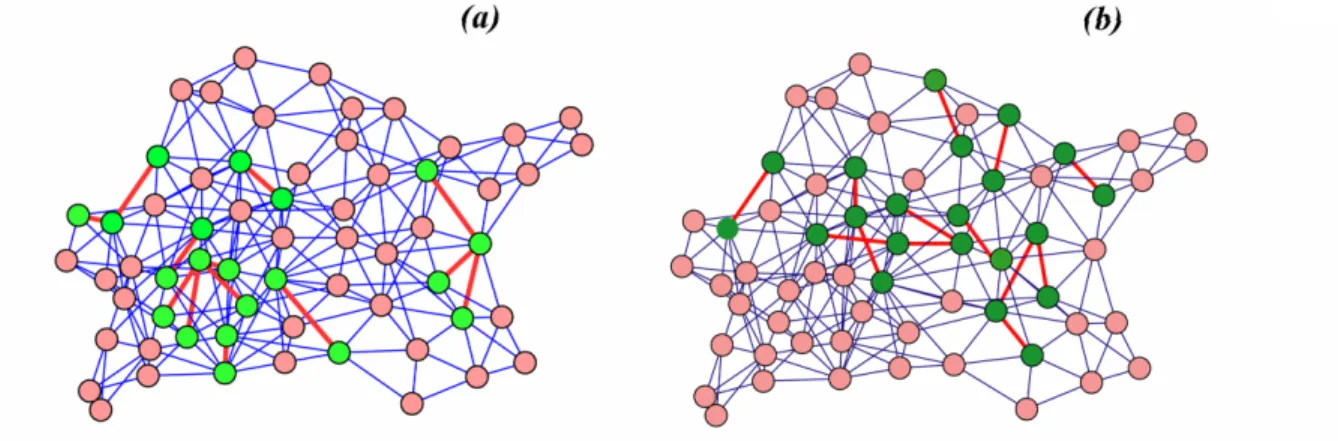
Graphs are mathematical structures used to model pair-wise relations between objects(Diestel, 2005; Albert and Barabasi, 2002). A graph is composed of a collection of nodes and a set of edges that connect pairs of nodes (Figure 1.6). A graph is called undirected if there is no distinction between the two nodes associated with each edge; or directed if its edges are directed from one node to another. A graph is called un-weighted if each edge is assigned with equal weight; or weighted if edges in the graph are assigned with different weights. A path in a graph is a sequence of nodes in which each node is connected to the next node in the sequence by an undirected/directed edge. The length of a path is defined as the total number of edges that are traversed along the path in an un-weighted graph, and the sum of the weights of the edges in a weighted-graph, respectively. A sub-graph of a given graph consists of a subset of nodes and the edges that connect between these nodes in the graph (Figure 1.6). Graph theory has important applications in a wide range of scientific problems. For example cellular metabolism has been modeled using graph theory where each

FIGURE 1.6. A sample graph and two sub-graphs are shown where the nodes and the edges of

CHAPTER 2

COMBINING HYDROGEN EXCHANGE DATA AND COARSE-GRAINED

SIMULATION TO CHARACTERIZE FOLDING INTERMEDIATE OF FAT DOMAIN

Introduction

Focal adhesion kinase (FAK) is a non-receptor tyrosine kinase that is expressed in most tissues and is regulated by integrin-dependent cell adhesion(Parsons, 2003). FAK functions in the control of several important biological processes, e.g. cell migration and

apoptosis(Schaller, 2001) and FAK is over-expressed in many forms of cancer. The correct localization of FAK to focal adhesions is required for integrin-dependent regulation of FAK and for FAK to direct tyrosine phosphorylation of downstream substrates. The C-terminus of FAK contains a focal adhesion targeting (FAT) domain, which is a four-helix bundle

structural motif that is responsible for subcellular localization of FAK.

Results from these studies suggest that the region around Y926 must adopt an extended conformation for phosphorylation and association with Grb2. There has been speculation (Arold et al., 2002; Liu et al., 2002; Prutzman et al., 2004) that for phosphorylation of Y926 and subsequent Grb2 binding to occur, the FAT domain must pass through an ‘open’

conformation in which helix 1 extends from the four helix bundle allowing the region flanking tyrosine 926 to adopt the necessary conformation.

While X-ray crystal (Arold et al., 2002; Hayashi et al., 2002) and NMR structures (Liu et al., 2002; Prutzman et al., 2004) reveal a four helix bundle fold for the FAT domain, a second structure has also been described. One of the reported crystal structures (Arold et al., 2002) is a dimer that has undergone ‘domain exchange’, in which the N-terminus and helix 1 of one molecule associates with helices 2 through 4 of the other symmetry-related molecule. The formation of the domain-exchanged dimer was speculated to proceed through an intermediate state where helix 1 transiently separates from the core bundle(Arold et al., 2002). The

Although weakly-populated protein-folding intermediates are often difficult to structurally characterize, hydrogen exchange methods have proven to be a powerful technique for identifying and characterizing kinetic and equilibrium folding intermediates (Bai et al., 1995; Chamberlain et al., 1996), but are limited in their ability to describe the structure of the intermediates. By combining hydrogen exchange data with discrete molecular dynamics (DMD)(Dokholyan et al., 1998) simulations, we have been able to capture structural details of the intermediate state ensemble for FAT domain folding, which has allowed us to reconstruct the conformers that we believe are important for FAK signaling through the FAT domain.

Material and methods

Hydrogen exchange protection factor

The relationships between the hydrogen exchange rates, transient unfolding mechanisms, and the structural stability of proteins have been previously described (Bai et al., 1994; Maity et al., 2003). The exchange rates of backbone amide protons are commonly expressed as protection factors, Pf = krc/kex, where kex is the experimentally measured hydrogen exchange

rate and krc is the intrinsic rate of hydrogen exchange in the unstructured protein. Protection

factors can be calculated using the method presented by Bai and coworkers (Bai et al., 1993). In the EX2 limit, usually satisfied when the structure of the protein is stable, the protection factor is equivalent to the equilibrium constant for the unfolding transition that makes the amide hydrogen exchange-competent. In this case, the protection factors may be used to calculate the free energy of the structural opening event:

Here, NMR HX data were collected by Dr. Sharon Campbell’s lab(Dixon et al., 2004). The derived protection factors were used as experimental constraints in discrete molecular dynamics simulations of the FAT domain folding process.

Incorporating protection factors into the Gō Model

In brief, the protection factors obtained from hydrogen exchange experiments can provide the free energy associated with the stability of the protein at each amino acid residue,

Discrete Molecular Dynamics Simulations

Interaction model

A discrete molecular dynamics (DMD) algorithm (Dokholyan et al., 1998; Smith et al., 1997; Zhou et al., 1997) was used to study the folding thermodynamics of the FAT domain, as DMD simulations have proven to be very useful in the study of folding kinetics

(Borreguero et al., 2002; Ding et al., 2002a; Zhou and Karplus, 1999) and aggregation of proteins (Ding et al., 2002b; Smith and Hall, 2001). The FAT domain was modeled using the ‘beads-on-string’ method developed by Ding et al. (Ding et al., 2003),with ‘beads’

corresponding to the Cα, Cβ, N, and C’ atoms. During the simulation, distance and angle constraints are maintained between the ‘bead’ atoms. The lowest eergy solution structure, determined by NMR (Prutzman et al., 2004), was used as the native structure and the Gō

potentialwas employed to model the interaction energy between native contacts. The non-bonded interactions were only assigned between Cβatoms (Cα for Gly) of residues i and j

(|i-j|>2):

ij

V

, (2.2)

⎪ ⎩ ⎪ ⎨ ⎧ > − < − < ≤ − ∞ + = b r r b r r a a r r V j i j i ij j i ij | |, 0 | | , | |, γε

were separated by more than 7.5 Å in the native state. The depths of the attractive square-well, εij in Equation 2.2, are equal in the unscaled Gō model, whereas in the scaled Gō

model,εij is assigned different strengths according to experimental data, as described below.

Scaling Gō model potentials using experimental protection factors

Since the measurements of the protection factors were performed under conditions where the folded state is dominant, we expect that hydrogen exchange for most of the residues is governed by the local fluctuation around the native structure. In the EX2 limit, where the protection factors can be used to determine the free energy associated with local protein stability, the measured protection factors can be related to the Gō model interaction energy according to Equation 2.3:

ln F

i ij ij

j j

P ≈

∑

f ε ≈

∑

εij , (2.3)

where the summation is taken over all residues j forming native contacts with the residue i,

and represents the probability of contact formation between residues i and j in the native state ensemble. We expect that the values of are approximately 1. Thus, in Equation 2.3, the protection factor reflects the heterogeneity in the contact energies.

F ij f

F ij f

The experimental protection factors were quantitatively determined for the subset of residues that could be monitored in real time. While some of the remaining residues could be approximated based on the CLEANEX-PM experiments(Hwang et al., 1997; Hwang et al., 1998), we did not calculate protection factors for residues that were not assigned in the 1

exchange rate using the experiments performed. So, to determine the set

{ }

εij that is most

consistent with the experimental data, a cost function was constructed that was minimized using Monte Carlo Metroplis algorithm(Binder, 1995):

(

)

2

2

ln , 0.1

i

F ij ij ij _all ij

all j

measured

W = ⎛_⎜ P − ε ⎞_⎟ + ε − ε ε ≥

⎝

∑

⎠ (2.4)

In the first term, the summation of j is taken over residues forming native contacts with i. <...>measured is the average taken over all the residues i with measured protection factors. For

residues that were observed using the CLEANEX-PM experiment(Hwang et al., 1997; Hwang et al., 1998), a small protection factor was assigned with a value of 10, as the results are not sensitive to the exact magnitude of this value. In the second term, <…>all is the

average taken over all the native contacts. The purpose of including the second term was to determine the pair-wise contact energies for residues that were not directly constrained by available experimental data, such as contacts between residues in which neither member of the pair has a measured or approximated protection factor. All native contact energies were constrained to have a minimum attraction interaction of 0.1.

Results and discussions

Scaled Gō model

The native contacts that were strengthened in the scaled Gō model are shown in the lower right triangle of Figure 2.1. After generating a set of scaled contact potentials

{ }

εij (as

described in Methods), we verified that our set was consistent with the experimental protection factors. Therefore, the contact frequencies, F, from the trajectories at low

simulation temperature, where the folded state is highly populated, were combined with the potentials

{ }

εij set according to Equation 2.3, to produce calculated protection factors.

FIGURE 2.1: Energy map for the FAT domain. Contact map for the native state of the FAT

domain with the pair wise contact potentials, scaled from the HX protection factors, shown in

the lower right triangle. The energy scale for the contact potentials is in units of ε.

The calculated protection factors show a strong correlation to the experimental protection factors for the FAT domain (Figure 2.2) with a correlation coefficient of 0.99. In contrast, if the set of unscaled contact potentials is used instead of the scaled set, the correlation

coefficient is only 0.07. The set of scaled contact potentials produced from the Monte Carlo minimization of the cost function (Equation 2.4, see Methods) therefore represents an accurate incorporation of the experimental protection factors into the DMD simulations.

exchange experiments were conducted or whether the EX2 limit was satisfied. Contact energies for each of these proteins were scaled according to their experimental protection factors, and then reconstituted in the form of calculated protection factors. Strong correlations were observed between the experimental and calculated protection factors (Figure 2.2) for all three proteins, with correlation coefficients similar to that obtained for the FAT domain. These results verify that our method for scaling the contact potentials is self-consistent.

FIGURE 2.2:Correlation between experimental and calculated protection factors. Correlation

plot comparing the experimentally determined protection factors with the reconstituted

protection factors after the Monte Carlo scaling of the pair wise contact potentials of the FAT

domain. The algorithm was applied to three other well characterized proteins: barnase, mutant

Recently, Vendruscolo and coworkers (Vendruscolo et al., 2003) have proposed a phenomenological approach to utilize hydrogen exchange data to bias the sampling in conformational space toward rare fluctuations of native proteins. In contrast, our method is intended to refine the interaction model with HX data so that we can better characterize the energetics underlying the folding process. Using this method, we are able to reconstruct particular ensembles at a given temperature and also characterize the thermodynamics and kinetic parameters of the FAT domain based on the rapid DMD simulation algorithm.

The temperature dependence of the average potential energy, derived from the scaled Gō

model simulation of the FAT domain, is shown in Figure 2.3. At low temperatures (T << 1, where the temperature is in reduced units of ε/kB), the FAT domain exists predominately in

its native folded state, whereas at high temperatures (T > 1), it is present mostly in an unfolded state. The sigmoidal curve shows a large increase of potential energy with the increase of temperature, which indicates a highly cooperative step in the transition. The shape of the curve alone does not provide the number of states there are at a given

FIGURE 2.3: The folding trajectory for the scaled DMD simulations. The folding trajectory of

the FAT domain from DMD simulations using the Go model with the pairwise contacts scaled

to agree with the experimentally determined protection factors. Error bars are shown

depicting the standard deviation. The temperature of the simulation and the total energy of the

protein are shown in reduced units based on the potential energy of the protein’s native

contacts, ε.

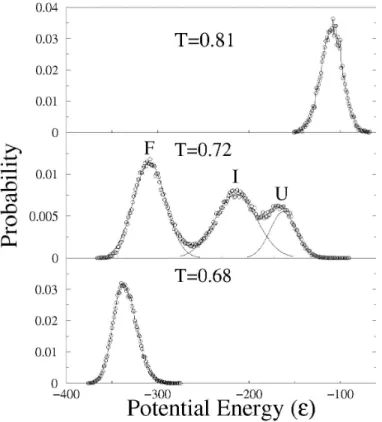
and a Gaussian fitting, used to determine the relative distribution of the states, shows that the intermediate state is significantly populated near the midpoint of the transition.

FIGURE 2.4: The probability distribution at three simulation temperatures. The probability

distribution of the total potential energy for the FAT domain, based on the summation over all

pair wise contacts, for three simulated temperatures along the folding transition. At T = 0.68

(bottom panel) the distribution of states is concentrated in a single distribution, with an energy

value near the native, folded state of the protein. As the simulated temperature is raised to 0.72

(~TM, middle panel), three distinct distributions are apparent: a native-like folded (F) state, an

intermediate (I) state, and a largely unfolded (U) state. A Gaussian fitting was used to

determine the relative distribution of the three states. Near the end of the transition (top panel),

T = 0.81, a single distribution is observed with an energy that is near the fully denatured state of

The FAT folding intermediate

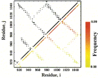
The intermediate state is not a discrete structure, but an ensemble of conformations that have potential energies that are distinct from the ensembles of the folded and unfolded states. There are two main characteristics of the intermediate detected by the scaled Gō model simulations of the FAT domain: 1) helix 1 separates from the helix bundle and 2) helix 1 loses helical structure. The frequency map for the intermediate state at T=0.72 is shown in the lower right triangle of Figure 2.5. The frequency map indicates the probability that a contact that exists in the native state, is being made at the given temperature of the simulation. Inspection of the intra-helix (along the diagonal) and inter-helix (perpendicular to the

diagonal) contacts, indicates that contacts made by helix 1 (residues 924-943) occur with lower frequency than the contacts made by residues in the other helices.

FIGURE 2.5: Frequency map for the intermediate ensemble. Contact map for the FAT domain

with the lower right triangle showing the frequency of the contacts in the intermediate ensemble

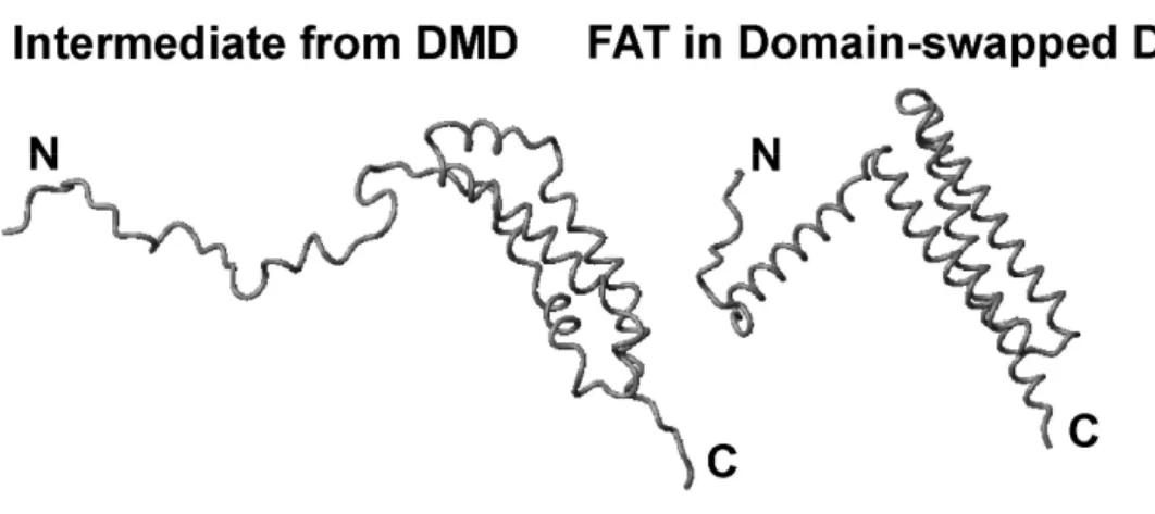
A single FAT domain molecule from the domain-swapped dimer structure (Arold et al., 2002) is shown next to a snap shot of the folding intermediate ensemble produced by the scaled Gō simulations in Figure 2.6; both structures share the characteristic of having helix 1 extended from the helix bundle. The intermediate structure is weakly populated at

temperatures that stabilize the four helix bundle fold, but increases in the DMD simulations when the temperature of the simulation is raised sufficiently. The domain swapped dimer structure was produced from crystals at room temperature (Arold et al., 2002), which

suggests that helix 1 transiently extends from the helix bundle at temperatures well below the melting temperature (TM = 83.4 at pH = 6.0, unpublished) and, consequently, allows the

domain exchanged dimer to form. Crystals of the domain-swapped dimer only appeared after three months, leading the authors to speculate that helix-exchanged molecules represent a minor population of the FAT domain. Although a domain-swapped dimer form of the FAT domain has been characterized, there is little evidence to support a role for a FAK dimer in vivo(Arold et al., 2002). As such, the FAT domain swapped dimer may be a byproduct of the FAT domain sampling a more ‘open’ intermediate which becomes populated at

concentrations used for X-ray crystallization. In contrast, mounting evidence suggests that helix 1 is conformationally dynamic, and conformational changes in helix 1 are important for phosphorylation of Y926 by Src, recognition by Grb2, initiation of MAPK signaling,

FIGURE 2.6: Comparison of the FAT domain intermediate from DMD simulations with the

domain-swapped dimer. DMD simulations on the FAT domain of FAK produce an ensemble of

structures for the folding intermediate. A single representative structure from the ensemble is

shown for comparison with a single molecule from the domain-swapped dimer crystal structure

(1K04) of the FAT domain. In both structures, helix 1 has separated from the helix bundle and

in the intermediate structure this is accompanied by the loss of helical character in helix 1. The

figure was prepared using MOLMOL.

The scaled Gō model simulations of the FAT domain reveal a folding-intermediate ensemble in which helix 1 is less structured and separates from the helix-bundle. Although the HX data indicates that residues in helix 1 are less protected than residues in helices 2-4, the HX data alone cannot confirm the presence intermediate state. Hydrogen exchange experiments as a function of chemical denaturant are able to detect cooperative units of unfolding (Bai et al., 1994) and subglobal unfolding, and have been employed to demonstrate sub-global unfolding in the four-helix bundle protein, cytochrome b562(Fuentes and Wand,

not necessary for our method, since scaling the native contacts was based solely on the effective exchange rate. Furthermore, using our scaled Gō model simulations, we were able to both identify cooperative units of unfolding and reconstruct coarse structures of the intermediate state.

The general features of this intermediate state are consistent with our recent solution structural studies of the FAT domain, in which line-broadening associated with NH

resonances in and around helix 1 and 2, led us to propose that a proline-rich ‘hinge region’ in the FAT domain produces strain resulting in enhanced conformational dynamics of helix 1 (Prutzman et al., 2004). Moreover, the intermediate state ensemble detected by our

DMD/HX approach is consistent with the FAT domain ‘sampling’ a more open state that leads to formation of a domain-swapped dimer(Arold et al., 2002). The region of the FAT domain that is exposed in this intermediate state ensemble, i.e., helix 1, has been shown to play a role in FAK phosphorylation, paxillin binding and FAK localization.

The Role of the Open and Closed Conformers of the FAT Domain

Results from this study combined with our previous observations (Prutzman et al., 2004) support the existence of ‘open’ and ‘closed’ conformations of the FAT domain. The four-helix bundle (closed conformation) of the FAT domain appears important for two distinct, yet related processes: paxillin binding and targeting FAK to focal adhesions. Recent

targeting of FAK show a strong correlation (Chen et al., 1995; Tachibana et al., 1995), studies of FAK mutants have revealed that paxillin-binding is dispensable for localizing FAK to focal adhesions (Cooley et al., 2000). It has therefore been suggested that paxillin-binding represents one mechanism for localizing FAK to focal adhesions and that alternative

mechanism(s) exist (Cooley et al., 2000). One possible alternative mechanism involves binding of the focal adhesion protein talin (Chen et al., 1995) to the FAT domain, which may facilitate the targeting of FAK to focal adhesions. Interestingly, mutational analyses indicate that while paxillin requires an intact FAT-structure for binding, talin does not (Chen et al., 1995; Hayashi et al., 2002). Therefore, the ‘closed form’ of the FAT domain may be important for targeting FAK to focal adhesions through a paxillin-binding mechanism.

conformational changes required for phosphorylation at Y926 are likely to disrupt paxillin FAT/HP2 interactions. Therefore, paxillin binding at HP2 and phosphorylation of Y926 are likely to be mutually exclusive events.

A previously reported double mutant, V955A/L962A, showed disruption of paxillin binding but retained the ability to target focal adhesions (Cooley et al., 2000). While the V955A/L962A double mutant does not cause significant structural alterations in the FAT domain (Prutzman et al., 2004), the mutations in helix 2 have been predicted to cause subtle perturbations in the 4-helix bundle core of FAT by disruption of specific hydrophobic interactions between helices 2 and 3. Our labs have shown that this double mutant exhibits an approximately 8-fold increase in dimerization (by gel-filtration) and a dramatic increase in Y926 phosphorylation invivo (Prutzman et al., 2004). The increase in dimerization suggests that the protein is more frequently sampling ‘open’ conformations that expose hydrophobic residues within the amphipathic helices (Prutzman et al., 2004). In the same study, it was shown that helix 1, when expressed as a GST fusion protein, was phosphorylated

approximately 8-fold more than a GST-FAT domain fusion protein (Prutzman et al., 2004). We have previously postulated that the increased phosphorylation, dimerization, and

disruption of paxillin-binding observed for V955A/L962A FAT variant may be the result of conformational dynamics involving helix 1 (Prutzman et al., 2004).

We have proposed a model for the role of FAT conformational dynamics in FAK-mediated cell adhesion and signaling processes, based on the available structural,

(pYNQV) for the SH2 domain of Grb2 (Rahuel et al., 1996), However, phosphorylation and subsequent binding requires a more extended conformation of helix 1 (Rahuel et al., 1996), and therefore helix 1 must have some degree of conformational flexibility to accommodate the required structural rearrangements (Arold et al., 2002; Liu et al., 2002). Grb2 binding at pY926 initiates signaling through the Ras/MAPK pathway. Therefore, transient population of the intermediate state conformers could favor the structural rearrangements of helix 1 that facilitate Grb2 activation of the MAPK pathway.

CHAPTER 3

CHARACTERIZING THE LARGE-SCALE STRUCTURAL DYNAMICS OF VINCULIN RELATED TO ITS ACTIVATION

Introduction

sites are occluded. Domain D2 stabilizes the pincer-like structure by forming extensive contacts with domain D3.

The activation of vinculin requires the release of the interaction between the D1 (residue 1-258) and Vt (residue 896-1066) domains, which is triggered by binding to different ligands. Early biochemical and structural studies established the role of an acidic phospholipid

PtdIns(4,5)P2 in disrupting the interaction between D1 and Vt by binding to Vt

domain(Gilmore and Burridge, 1996; Weekes et al., 1996; Bakolitsa et al., 1999). The release of the D1-Vt interaction further exposes cryptic binding sites in vinculin for other ligands, including talin, α-actinin, α-catenin, vasodilator-stimulated phosphoprotein (VASP), vinexin, ponsin, actin-related protein complex (Arp2/3), paxillin and actin(Zamir and Geiger, 2001). In contrast, the role of talin in releasing the head-tail interaction was uncovered more recently(Izard and Vonrhein, 2004; Izard et al., 2004). It was found that the binding of specific short talin peptides (~30 amino acids) to the D1 domain alone is sufficient for releasing intra-molecular head-tail interactions in the D1-Vt complex by provoking significant structural changes of the D1 domain, suggesting an alternative pathway of vinculin activation, in which PtdIns(4,5)P2 may not be required(Izard and Vonrhein, 2004; Izard et al., 2004). However, Bakolitsaet al.(Bakolitsa et al., 2004) and Gilmore and Burridge(Gilmore and Burridge, 1996) demonstrated that larger fragments of talin bind poorly to full-length vinculin in vitro. When PtdIns(4,5)P2 is added, binding strength increases four-fold(Gilmore and Burridge, 1996). Hence it is more likely that the activation of vinculin is achieved by a combinatorial binding of ligands rather than any single

Despite intensive biophysical and biochemical studies, a global and dynamic picture of vinculin activation is still lacking. Experimental characterization of the large-scale

conformational dynamics relevant to vinculin activation is challenging. Even using computational methods, the time-scale of the conformational dynamics and the size of vinculin are beyond the resolution capabilities of the current all-atom molecular dynamics simulation techniques. Hence, to uncover the large-scale conformational dynamics associated with vinculin function, we utilize rapid discrete molecular dynamics (DMD)(Dokholyan et al., 1998; Smith et al., 1997; Rapaport, 2004) techniques. We find distinct and

complementary roles of internal (inherent flexibility, domain-domain interactions within vinculin) and external (talin binding) factors in allosteric control of vinculin, suggesting possible mechanisms for vinculin activation.

Materials and methods

Homology modeling of missing loop structure

The conformation of a loop (856-874) is missing in the X-ray structure of vinculin. We use the biopolymer module of the program SYBYL to reconstruct the backbone

conformation of this loop. The reconstruction is based on homology modeling

method(Sanchez and Sali, 1997). By searching the structural homologues of this loop in the Brookhaven Protein Databank (PDB)(Berman et al., 2000), we use SYBYL to generate a candidate list of loop structures for reconstruction. From this list as the template for

We further add side chains to amino acids on the reconstructed backbone. We determine the optimal rotamer states of side-chains by a Monte-Carlo minimization procedure(Ding et al., 2006).

Protein and interaction model

We perform DMD simulations using a simplified two-bead protein model, in which each residue is represented by one backbone bead Cαand one side-chain bead Cβ(only Cα for Gly).

The detailed implementation of covalent bonds and constraints that maintain the geometry of each residue in the model can be found in Ref. (Ding et al., 2002a). In addition to the

covalent bonds and constraints, we use the Gōpotential(Abe and Go, 1981; Go and Abe, 1981) to model the non-bonded interactions within monomers. The chicken vinculin crystal structure(Bakolitsa et al., 2004) (PDB accession code 1ST6) with reconstructed loop is used as native structure to assign the Gōpotential. We also incorporate backbone hydrogen bonding interaction into the simulations (Ding et al., 2002b).

Thermodynamic and kinetic simulations

In thermodynamic studies, prior to the equilibrium simulations we perform simulations for 1x105 time units from the initial temperature T=0.1 to various target temperatures in the range between T=0.1 and T=2.0 (simulation temperature is in units of ε/kB, where ε is the

energy unit and k

B

B is Boltzmann’s constant). We then perform equilibrium simulations for

1x10 time units at corresponding target temperatures. In kinetic studies, we perform twenty unfolding simulations starting from the same native structure of vinculin but different initial velocities. In each kinetic unfolding simulation, we gradually (during 5x10 time unit)

6

increase the system temperature from T=0.1 to T=0.9. We then analyze the pattern of dissociations between domains and within domains during the course of unfolding.

Fraction of native contacts as a measure of dissociation magnitude

A native contact is defined to exist in a given conformation if the Cβ atoms of two residues

are within a cutoff distance (7.5 Å) both in this conformation and in the native structure. The cutoff distance used to define the native contact is the same as the one used to define

structure-based Gōpotential. The fraction of native contacts (Q) is defined as the ratio between the number native contacts in a given conformation and in the native structure. It takes the value ranging from one (when a protein adopts native structure) to zero (when a protein is fully-unfolded) and has been used as a reaction coordinate in the study of protein folding(Onuchic et al., 2000).

Characterization of the principal motions near the native state

We use essential dynamics to characterize the principal motions near the native state. The essential dynamics(Amadei et al., 1993; Ichiye and Karplus, 1991) is based on the

diagonalization of the covariance matrix constructed from fluctuations of Cα atoms in the

simulation trajectories in which the overall translation and rotation have been removed: >

− −

=<(Xi Xi,0)(Xj Xj,0)

M (3.1)

Xi(Xj) in Eq.(3.1) are the separate x, y, z coordinates of the ith (jth) Cαatom (i,j=1...N, N is

the total number of Cα atoms) fluctuating around its average Xi 0. The average is taken over

the protein undergoes conformational fluctuations near native state. The diagonalization of Eq.(3.1) yields a set of eigenvectors (describing directions in the high-dimensional

configurational space) and eigenvalues (represent the mean square fluctuation of the total displacement along the eigenvectors). The first few eigenvectors with the highest eigenvalues describe principal motions. Motions along these eigenvectors are mainly large anharmonic fluctuations and generally can be linked to the biological functions of the proteins. The motions described by eigenvectors with small corresponding eigenvalues represent harmonic (Gaussian) fluctuations, which are thermal fluctuations in nature.

Simulation of the interaction between vinculin binding site peptide from talin and vinculin

To investigate the role of talin binding in vinculin activation, we perform simulations of the binding of vinculin binding site (VBS1, residue 605-636) from talin to vinculin. We model

the interaction between vinculin and VBS1 by constructing the following effective potential: (3.2) ), ( E E E E j , i 1 VBS 1 D ij j , i bound 1 D ij j , i free 1 VBS ij ij free vinculin ij ) 1 VBS vinculin ( eraction int free 1 VBS free vinculin tot ∑ ∑ ∑ ∑ − − − − − − − + + + = + + = Δ Δ α Δ Δ

where and are the Gō-like pair-wise contact energies corresponding to the free state of vinculin(Bakolitsa et al., 2004) (PDB accession code 1ST6) and the free state of VBS1(Papagrigoriou et al., 2004) (PDB accession code 1SJ7), respectively. Matrices

and are the Gō-like contact energies of the VBS1-bound state of D1 domain and between D1 domain and VBS1 that are assigned based on the D1-VBS1 complex structure(Papagrigoriou et al., 2004) (PDB accession code 1TO1). The inclusion of contact energies for the VBS1-bound state of D1 domain serves to effectively account for the conformational change of D1 upon VBS1 binding. For units that dissociate from each other,

} { vinculin free

ij

−

Δ { VBS1 free}

ij

−

Δ

} { D1 bound

ij

−

Δ { D1 VBS1}

ij

−

it is important to scale effective energy contribution to reflect the additional translational entropy gained by interacting domains. Parameter α is such scaling coefficient, the range of which is determined by consistency of simulations with experimental observations. More specifically, we determine the range of α by satisfying the following two conditions to be in agreement with experimental observations: first, without VBS1, the native state of the free D1 is the most stable state (RMSD from free D1 and VBS1-bound D1 structure are <2.4Å and >3.0Å, respectively); second, with VBS1, the experimentally-determined D1-VBS1 complex is the most stable state at low temperatures (RMSD from complex structure is <2.4Å). With the determined range of α between 0.65 and 0.72, we then perform simulations in the presence of both VBS1 and vinculin at various temperatures. The simulation results are not sensitive to the exact value of α within the determined range. To improve the efficiency of simulation, we constrain the distance between Cβ atoms of residue 616ALA of VBS1

peptide and residue 15PRO of D1 domain within 12 Å (these two atoms are within 7.5 in the native D1-Vt complex) so that the VBS1 and vinculin are spatially close to each other.

Results and discussion

The principal motions near the native state

The principal motions that dominate conformational fluctuations in the vicinity of the native state of proteins often recapitulate the structural dynamics underlying their biological

use essential dynamics analysis(Amadei et al., 1993; Ichiye and Karplus, 1991) (Methods) to find the principal motions of the polypeptide chain. The first dominant mode is characterized by a breathing motion between two elements of vinculin structure (Figure 3.1a). One such element consists of the end of the proline-rich linker region (Figure 3.1) and the structural region from Vt helix bundle that is spatially proximal to the proline-rich linker region. The other element contains the structural region from D3 that is in spatial proximity to Vt and one of the two helix bundles from D2 that has extensive contacts with D3. The first dominant mode also involves a global twisting motion that occurs between two helix bundles within D2. The second dominant mode is highlighted by a “holding” and “releasing” motion between Vt domain and pincer-like structure formed by D1, D2 and D3 (Figure 3.1b). The “holding” and “releasing” is synergized between the structural region from the Vt that is spatially proximal to D1, the structural region from D3 that is close to Vt and the middle region in the D2 structure (Figure 3.1b). The third dominant mode involves the nearly-parallel rotation and twisting of D1, D2 and Vt (Figure 3.1c), reflecting the flexibility along the orthogonal directions distinct from the first two dominant modes. The interaction

FIGURE 3.1. The native structure of full-length vinculin is shown in the left of Figure 1. It

comprises of five distinct domains and one proline-rich linker region connecting the fourth and

the fifth domain: D1, 6–252 (blue); D2, 253–485 (yellow); D3, 493–717(red); D4, 719–835 (cyan);

proline-rich linker region (838-890) consists of a proline-rich region (838-878) and a “strap”

(878-890); D5 (vinculin tail), 896–1066 (green); The pincer-like structure formed between D1,

D2 and D3 is illustrated in the bottom-right beside the native structure. All the protein

structures are made with PYMOL. The first three dominant modes of principal motions near

the native state of vinculin are illustrated as follows: a, the first dominant mode; b, the second

The thermal “melting” of intra and inter-domain interactions

To further characterize inter- and intra-domain structural plasticities of vinculin that contribute to its function, we study the thermal “melting” of inter and intra-domain

interactions in vinculin. We perform equilibrium simulations at various system temperatures ranging from T=0.1 to T=2.0. At each temperature, we use the fraction of native contacts (Methods) to quantify the magnitude of dissociations between and within domains. We plot the fractions of inter-domain and intra-domain native contacts as functions of temperature (Figure 3.2). We find that dissociations between most domains (D1-Vt, D3-D4, Vt-D3, D2-D3, Vt-D4, D1-D3) exhibit cooperative changes with increasing temperatures. In contrast, the association between D1 and D2 domain shows a gradual, rather than cooperative,

decrease when temperature increases (Figure 3.2a). In addition, we find that the associations between Vt and D3 domain are completely lost at the temperatures where the majority of the contacts between other domain pairs are kept, indicating that the effective interaction

between the Vt-D3 pair is weaker compared to other pairs (Figure 3.2a). Noticeably, the significant dissociations between the tail domain and the “pincer” formed by D1-D3 and between the constituent domains of the “pincer” occur in the temperature range near the midpoint ( ) of thermal denaturing curve of the whole vinculin (curve not shown). This observation indicates that the interactions between these domains contribute

cooperatively to the stability of the whole vinculin.

75 . 0 ≈

T

As temperature increases, the dissociations between domains are followed by the