The Impact of Roads on Land-Use Change in Ethiopia: Evidence from Satellite Data
By: Ariana Brynn Vaisey
Honors Thesis
Economics Department
University of North Carolina at Chapel Hill
April 2016
Approved:
___________________________
Abstract
Using satellite-based land cover data for Ethiopia, I examine the relationship between travel costs and the spatial allocation of economic activity. In analyzing a cross-section of land cover data for all of Ethiopia in 2005/2006, I find that proximity to market is positively
Acknowledgements
I would like to thank my supervisor, Dr. Simon Alder, for providing invaluable guidance in formulating a research question, using geographic information systems software to collect data, and building a model to test my hypotheses.
I would like to thank Dr. Klara Peter, my faculty advisor, for ensuring that I stayed on track with early deadlines throughout the process and for challenging me to answer questions with new empirical methods learned in the seminar.
1. Introduction
Roads and other transportation infrastructure affect land use through their impact on
reducing transportation costs. When firms and commuters make a decision about where to live or
locate their operations, they face tradeoffs between land rents and the cost of transportation to
market, among other factors. At a given distance to market, transportation is so expensive that it
becomes unprofitable to operate or live in an area (von Thünen, 1826; Alonso, 1964). Therefore,
reducing transportation costs expands economic activity by increasing market access (Donaldson
& Hornbeck, 2016). This paper uses empirical methods to examine the effect of transportation
infrastructure on the spatial distribution of land cover types. Land cover reflects land use and
thus the forms of economic activity that are taking place in a given area; for instance, agricultural
activity can be identified by observing the location and extent of farmland. In this paper, I use
Ethiopian data to study whether road construction and upgrading leads to a greater allocation of
land to agriculture versus other uses (vegetation, urban or industrialized area), and the magnitude
of this effect.
Historically, most of the literature discussing the effect of transportation infrastructure on
the spatial distribution of economic activity has been theoretical in nature. However, the number
of empirical studies in this area is expanding. Recent contributions consider suburbanization in
the United States (Baum-Snow, 2007), trade and income in India (Donaldson, forthcoming),
GDP in peripheral regions in China (Faber, 2014), and the size of the eighteenth-century
American agricultural sector (Donaldson & Hornbeck, 2016). My paper adds to this literature by
examining data from the African continent, where little empirical work has been done, and by
Ethiopia makes an interesting case-study on the economic effects of transportation
infrastructure because of its geography, level of development, and ongoing expansion of the
transport infrastructure network. A circular rural country with a core primate city, Addis Ababa,
Ethiopia closely resembles the “Isolated State” developed in von Thünen’s early model of
agricultural land. Lacking a domestic coastline, Ethiopian goods destined for export are
transported to ports in Djibouti, usually through Addis Ababa. Thus, the country is an ideal place
to empirically test established theories of economic geography. Additionally, Ethiopia is a rural,
fast-growing country going through a period of significant investment in transportation, making
it a suitable location for a study on the impact of road construction and upgrading on the
allocation of land to different economic activities.
Few studies make use of new satellite-based data to analyze land use change associated
with transportation infrastructure. Remotely-sensed land cover data is advantageous because it is
available at relatively high spatial and temporal resolutions over a wide geographic area,
allowing changes in land use over time to be observed in detail. Over the last decade, satellite
imagery has become more publically accessible and new algorithms and improved processing
power have made it possible to extract increasing amounts of data. In this paper, I employ
satellite data to classify land cover across Ethiopia and track changes in land cover and
associated land use over time, in the proximity of newly built or upgraded roads.
This paper answers the question of how road construction affects the spatial distribution
of economic activity by studying the location of land devoted to vegetation, agriculture or urban
area in Ethiopia. In the first part of the paper, I use Ethiopia-wide road network data for 2004 and
land cover data for 2005/2006 to examine in the cross-section the distribution of land cover types
explore in detail the changes in land cover before and after the construction a specific segment of
road network, the Addis Ababa-Adama Expressway opened in September 2015. I compare the
changes in land cover within an inner buffer of the expressway as compared to land in an outer
buffer of the same expressway. This allows me to employ a difference-in-difference approach to
estimating the causal effect of transportation infrastructure on economic activity as measured by
land cover.
The paper is structured as follows: Section 2 describes the background in Ethiopia and
policy applications of this research. Section 3 discusses the relevant literature. Section 4 presents
the theoretical model. Section 5 presents the empirical model. Section 6 describes the data
collection. Section 7 presents the data and descriptive statistics. Section 8 discusses the results.
Section 9 concludes.
2. Background
Based on theory about the positive relationship between reduced transportation costs and
economic growth, many countries and development agencies have pursued an
infrastructure-centered approach to development that includes massive road network expansions, including
China and Ethiopia (Fourie et al., 2015). Since launching the Road Sector Development Program
(RSDP) in 1997, Ethiopia has increased the length of its federal and regional road network
(asphalt and gravel roads) from 26,500 km to 63,604 km in 2015 (Ethiopian Development
Research Institute, 2011; Federal Republic of Ethiopia, 2016). Including all-weather woreda
roads, Ethiopia’s total road network reached 110,414 km in 2015, more than double the length in
2010 and resulting in a decrease in the average time to reach the nearest all weather road from
Transportation Plan (GTP II), the country plans to further increase the all-weather road length to
220,000 in 2019/2020 (Federal Republic of Ethiopia, 2015). In this paper, I provide empirical
evidence that rigorously evaluate the impacts of transport infrastructure on economic activity in
Ethiopia, as measured through land cover and how it changes over time.
3. Literature Review
A large body of theoretical literature examines the relationship between transportation
infrastructure and economic activity. The theoretical literature establishes a tradeoff between
transportation costs and land rents, which influences the spatial allocation of economic activity
depending on the relative costs of transportation associated with land uses. Additionally,
empirical literature supports the hypothesis that a decline in transportation costs leads to an
increase in economic activity, including the area of agricultural land.
The model used in this study is based in Johann H. von Thünen’s model of agricultural
land use, published in his 1826 treatise The Isolated State, which founded the field of spatial
economics and continues to play a central role in urban theory. Von Thünen imagined a
featureless plane with a town at the center supplied by farmers in surrounding fields, who
cultivate crops that only differ in yield per acre and transportation costs. Land rents decline with
distance from the city center, so farmers face a tradeoff between land rent and transportation
costs. “Bid-rent” curves define the rent farmers are willing to pay for land to grow each type of
crop at a given distance from town, and form the rent gradient. At the outermost edge of
cultivation, land rents fall to zero.
Following a resurgence of interest in spatial economics, later theoretical work extended
(1969), and Mills (1972) developed a monocentric city model wherein workers commuting to a
sole center face a tradeoff between the price of housing and transportation. This applies von
Thünen’s theory to economic activities other than agriculture. In my model, I will consider the
effect of transportation costs on the margins between vegetation, agricultural, and urban land
cover/use.
Krugman (1991) sought to explain the formation of a town or city itself in his seminal
paper on new economic geography. Using a simple two-region model, Krugman proposed that
the interaction of economies of scale and transportation costs can cause manufacturing activity to
start to concentrate in one region and induce a positive feedback loop that generates further
divergence in types of economic activity between regions – creating agglomeration. In my paper,
I do not seek to explain the formation of urban centers such as Addis Ababa. However,
Krugman’s analysis affirms the premise that transportation costs are important for the spatial
allocation of economic activity. Krugman’s model also helps to explain the patterns of land
cover/use observed in Ethiopia, as will be discussed in the results section.
Eaton and Kortum (2002) develop a Ricardian model of international trade that
incorporates a role for geography, including transportation costs, as a barrier to trade. This
approach provides a framework to simultaneously confront the role of geography and technology
in economic activity. Donaldson and Hornbeck (2016) use an Eaton-Kortum model to measure
market access and its impact on agricultural land values in the United States, as discussed later in
this literature review. This methodology also motivates own calculation of market access.
Economic theory has been applied to a number of empirical studies on the economic
effects of transportation infrastructure, though relatively few focus on land use. Chomitz and
construction on deforestation using von Thünen-type models where land operators allocate land
use to maximize expected net benefits from output. Following an iceberg model of transportation
costs, they assume the value of agricultural output declines with distance to market. Reducing
distance to market then increases the potential rent from agriculture and promotes the expansion
of farming activity. Using data from Belize, Mexico, and Brazil the authors find that road
construction causes the conversion of forest to agriculture (Chomitz and Gray, 1996; Nelson and
Hellerstein, 1997; Pfaff, 1999). As in my analysis, these authors rely on GIS methods using
satellite data to classify land cover types. I add to this literature by using a much larger sample
area – the whole of Ethiopia – (previous studies use pixel-level data only for a small, regional
sample area or else aggregates data to the county level). I am able to do this in part because of
new satellite data available, such as the European Space Agency’s GlobCover project that began
in 2005 and provides land cover data for the whole world.
Donaldson and Hornbeck (2016) use a general equilibrium model from trade theory to
estimate the impact of railroad construction in nineteenth-century America on agricultural land
value through increased market access. The authors link half of the estimated increase in
agricultural land value to agricultural extensification. Drawing from Donaldson and Hornbeck
(2016), I consider market access as an explanatory variable for land use. This adds to previous
literature on land cover change that only considers road densities or distance to the nearest road,
village, or capital (Chomitz and Gray, 1996; Nelson and Hellerstein, 1997; Pfaff, 1999).
Existing studies on transportation infrastructure expansion in Ethiopia focus on poverty
reduction and business growth as measures of economic activity. Dercon, Hoddinott and
Woldehanna (2012) find that reducing the distance on the road network to the nearest small town
2009 in Ethiopia. Shiferaw et al. (2015) estimated that a 1-percent reduction in travel time to
major commercial destinations in Ethiopia increases the size of new entrants by 3-percent, using
cross-sectional data on firms and transportation networks. My study is different in that it draws
from data points covering an entire area, not just towns and cities, and allowing the impact of
transportation infrastructure on peripheral areas to be included. Also, my study looks specifically
at effects on agricultural activity, which has not been studied previously in Ethiopia to my
knowledge. The vast majority of Ethiopians earn their livelihood from agriculture and
agricultural products drive Ethiopian GDP (Lavers, 2012), making this an important sector to
understand and analyze in a development context.
4. Theoretical Model
The theoretical model in this paper is based on von Thünen’s model (1826) and
applications of the von Thünen model to deforestation by Chomitz and Gray (1996). Von
Thünen imagined an “Isolated State” where profit-maximizing farmers transport their goods
across land directly to a central city. This simplistic model in fact bears out very well in the
Ethiopian context. Ethiopia is a rural country, where 85 percent of the population depends
primarily on smallholder agriculture produced through household labor (Lavers, 2012). The
small surplus of crops feeds the urban population, and few agricultural goods are exported in
significant proportion (Lavers, 2012).1 This is in part due to high transportation costs to Djibouti
(Ethiopia is landlocked), which make exports often unprofitable (Dercon & Vargas Hill, 2009).
Ethiopia’s capital, Addis Ababa, is located in the geographic center of circular-shaped Ethiopia
and has a population 12 times the second-largest city, making it a quintessential primate city
(Wubneh, 2013). I am thus confortable using a model that tracks von Thünen closely.
Following von Thünen (1826) and Chomitz and Gray (1996), I assume that each parcel of
land has a potential for rent attached (the market value of output minus transportation costs).
Land users will devote land to the activity that gives the highest rent. Beyond a certain distance
from the city, any economic activity becomes unprofitable because of rising transportation costs
and the land is left undisturbed as natural vegetation. The derivation below follows that of
Chomitz and Gray (1996).
From Chomitz and Gray (1996), the return to a certain land use is the rent 𝑅!", given by
(1) 𝑅!" = 𝑃!"𝑄!"(𝑃!",𝐶!") −𝐶!"𝑋!"(𝑃!",𝐶!"),
where 𝑃!" is the output price, 𝑄!" is the quantity of output, 𝐶!" is a vector of input costs, and 𝑋!"
is a vector of inputs quantities, all for land use 𝑘 at parcel location 𝑖. A land parcel is allocated to
land use 𝑘 if this use gives the highest rent compared to all alternatives for that parcel:
𝑅!" > 𝑅!! for all ℎ≠ 𝑖.
In my model, I consider three possible types of land uses: idle (natural vegetation), agriculture,
and built-up/urban area.
I do not have data on location-specific prices and costs, since they are unobserved.
Therefore, I use a reduced-form model that takes observed determinants of price and productivity
as inputs. Following von Thünen (1826) and Chomitz and Gray (1996), I assume that spatial
differences in farm-gate prices are only due to differences in transportation costs to market, 𝐷!.
(2) 𝑃!" = exp [γ!!+γ!!𝐷!]
Using an iceberg model of transportation costs, I expect that output prices fall as access costs
increase (γ!! < 0). Here, we can think of output prices as those received by the land owner when
they sell their product to a truck driver at the land parcel location. The truck driver receives the
same price for all goods at the central market, so offers land owners less money for goods
produced at greater distances to market, in order to make up for transportation costs. The model
structure is based on an assumption of monopolistic competition.
Also, I expect that input costs rise (δ!! > 0) when land is devoted to a marketed output,
so that idle land could have zero access cost.
I use a Cobb-Douglas production function for output per unit of land that includes
parcel-specific geophysical factors 𝐺!" , such as soil quality and average rainfall, that effect land
productivity, from Chomitz and Gray (1996):
(3) 𝑄!" =𝐺!"𝑋!"!! [0< 𝛽 ! < 1]
𝐺!" = 𝜆!!𝐺!!!!"𝐺!!!!!…𝐺!"!!"
From equation (3), we have the demand for 𝑋:
(4)
𝑋!" =
𝐶!"
𝑃!"𝐺!"𝛽!
!/[!!!!]
Then, combining equations (1), (3), and (4):
(5) 𝑅!" = 𝑃!"𝑄!"−𝐶!"𝑋!" =𝑃!"𝐺!"𝑋!"!!−𝐶
!"𝑋!" =𝑋!"[𝑃!"𝐺!"𝑋!"!!!!−𝐶!"]
𝑅!" = 𝐶!"
!! !!!! 𝑃
!"𝐺!"𝛽! !
!!!!(!!!!)
!!
Thus, we see from the above equation that rent increases as output prices 𝑃 increase and
decreases as input costs 𝐶 increase, as expected.
(6) ln 𝑅!" = 𝛼!!+ 𝛼!!𝐷! +𝛼!!𝑙𝑛(𝑔!!)+⋯+𝛼(!!!)!𝑙𝑛(𝑔!")+𝜀!"
where, as before, 𝐷! represents distance to market along the road network and 𝑔!!… 𝑔!"
represent geophysical characteristics of the land parcel 𝑖.
For agricultural activity, I expect the coefficients on distance to be negative and the
coefficients on geophysical characteristics that increase productivity to be positive (Chomitz and
Gray, 1996). This is because it is more profitable to produce crops in areas with lower
transportation costs (higher farm-gate prices) and where agricultural productivity is higher. For
urban areas, I expect the same negative coefficient on distance but a smaller positive coefficient
on the geophysical characteristics, since the land is not farmed but proximity to agricultural areas
that supply the town is important to support the town’s population.
5. Empirical Model
I estimate the effect of roads on the allocation of land in Ethiopia using two empirical
models based on the theoretical framework described in the previous section. The first section a
is cross-sectional study, using data for all of Ethiopia in 2005/2006, and the second part is a
panel study that examines changes in land cover types before and after the construction of an
expressway, in the area surrounding the expressway.
In the first part of the paper, I estimate the probability of devoting parcel 𝑖 to land use 𝑘
using a multinomial logit model. I use a multinomial logit model because I am interested in the
probabilities associated with three possible discrete land cover outcomes: vegetation
(uncultivated land), agriculture, and urban area. I assume that expansions in the extent of
agricultural and urban area indicate increases in economic activity, and thus economic growth. It
agricultural intensification), since this is not possible to measure using my dataset derived from
satellite imagery. As discussed in later in my data section, because of the small number of
observations of urban area and likely under-estimation of this land cover type, I focus my
analysis on the transition from vegetation to urban area.
Logistic models require the assumption that the error terms are independent and
identically distributed (𝜀!"~ 𝑖𝑖𝑑) and follow a particular function form. The model is specified
by the following equation:
(7)
𝑃𝑟 𝑖 =𝑘 ! =
exp [ln (𝑅!")!]
exp [
! ln (𝑅!")!]
𝑃𝑟 𝑖=𝑘 !=
exp [𝜎!!"+ 𝜎!!𝐷!"+𝜎!!𝑙𝑛(𝑂!")+𝜎!!𝑙𝑛(𝐻!")+𝜎!!𝑙𝑛(𝑅!")+𝜎!!𝑙𝑛(𝐴!")+ 𝜎!!𝑙𝑛(𝑁!") ]
exp [
! 𝜎!!"+ 𝜎!!𝐷!𝑡+𝜎!!𝑙𝑛(𝑂!")+𝜎!!𝑙𝑛(𝐻!")+𝜎!!"𝑙𝑛(𝑅!")+𝜎!!𝑙𝑛(𝐴!")+ 𝜎!!𝑙𝑛(𝑁!")]
where 𝐷 represents distance to market (I use a variety of measures, described in the data section),
𝐶 represents the organic carbon content of the soil, 𝐻 represents the acidity (pH) of the soil and
𝑅 represents the long-term average annual precipitation at the land parcel, 𝐴 represents latitude,
and 𝑁 represents longitude (for rationale on the choice of controls, see below). I classify land
according to three potential uses: vegetation (uncultivated land), agriculture, and urban area. As
described by the theoretical model, the land user devotes the land at time 𝑡 to the highest rent
available in period 𝑡.
This model assumes that the construction or roads is exogenous to agricultural land use,
which is potentially a very strong assumption. In cases where roads are installed to curry political
favor, the assumption may hold true (Chomitz and Gray, 1996). However, if roads are
purposefully placed in more agriculturally suitable areas and the determinants of the suitability
are unobserved, the model may overstate the effect of distance to market on the probability of
indicators: organic carbon content and pH. These are together the best simple indicators of the
health status of soil (Nachtergaele et al., 2009). Moderate to high amounts of organic carbon are
associated with fertile soils, and acid to neutral soils are the best pH conditions for nutrient
availability and suitable for most crops (Nachtergaele et al., 2009). Additionally, I include a
variable for long-term average annual rainfall since Ethiopia is a drought-prone country and lack
of available water is a main constraint on the ability to grow crops. I also include controls for
latitude and longitude, and fixed effects for administrative region (zones).
In the second part of this study, I analyze the land-use change associated with the
construction of specific segments of road. Using panel data (compared to cross-sectional data in
the first section of the paper) helps to isolate the effects of road construction on land use
decisions by allowing me to control for unobserved time-invariant variables.
I use difference-in-differences to estimate the effect of road construction and upgrading
on agricultural land cover/use. As a treatment group, I use the land cover in an inner buffer of the
newly-constructed Addis Ababa-Adama expressway. My control group is an outer buffer of the
road. In September 2015, the Ethiopian government opened the Addis Ababa-Adama
expressway, the country’s first expressway and toll road. The six-lane expressway connects
Ethiopia’s two biggest cities – with link roads to major towns along the road – using advanced
technologies new to Ethiopia, such as traffic cameras and variable message signs, together with
interchanges, overpasses and underpasses. The expressway reduced travel time between Addis
Ababa and Adama to 40 minutes from around two hours using the previous paved road
(Embassy of Ethiopia in Belgium, 2014).
I estimate the proportion of the land devoted to agriculture as a function of being in an
(8) 𝑃𝑟 𝑖 =𝑎𝑔𝑟𝑖𝑐𝑢𝑙𝑡𝑢𝑟𝑒 != 1/[1+exp (−( 𝜎!+ 𝜎!𝑇𝑟𝑒𝑎𝑡! +𝜎!𝑃𝑜𝑠𝑡!+ 𝜎!(𝑇𝑟𝑒𝑎𝑡! ∗
𝑃𝑜𝑠𝑡!)+𝜎!(𝐴𝑟𝑒𝑎! ∗𝑃𝑜𝑠𝑡!)+𝜎!𝑆𝑜𝑖𝑙! +𝜎!(𝑆𝑜𝑖𝑙!∗𝑇𝑟𝑒𝑎𝑡!)+𝜎!(𝑆𝑜𝑖𝑙! ∗𝑃𝑜𝑠𝑡!)+
𝜎!(𝑆𝑜𝑖𝑙! ∗𝑇𝑟𝑒𝑎𝑡!∗𝑃𝑜𝑠𝑡!)+𝜀!"))]
where 𝑇𝑟𝑒𝑎𝑡! is a dummy for if the land parcel 𝑖 is in the treatment group, 𝑃𝑜𝑠𝑡! is a
post-treatment dummy, 𝐴𝑟𝑒𝑎! captures the percent of agriculture in a 2.5-kilometer buffer of land
parcel 𝑖, and 𝑆𝑜𝑖𝑙! represents the soil quality of land parcel 𝑖. The treatment group is the area of
land within an inner buffer (20km) of the Addis Ababa-Adama expressway and the control group
is the area of land within an outer buffer (40km) of the planned Addis-Ababa-Adama
expressway, excluding land in the inner buffer.
The average treatment effect on the treated (ATT) at the time of treatment is defined by:
(9) 𝜏 𝑇𝑟𝑒𝑎𝑡! =1,𝑃𝑜𝑠𝑡!= 1
= 𝐸 𝑌! 𝑇𝑟𝑒𝑎𝑡
! = 1,𝑃𝑜𝑠𝑡! =1,𝑆𝑜𝑖𝑙!,𝐴𝑟𝑒𝑎!
− 𝐸 𝑌! 𝑇𝑟𝑒𝑎𝑡
! =1,𝑃𝑜𝑠𝑡!= 1,𝑆𝑜𝑖𝑙!,𝐴𝑟𝑒𝑎!
where 𝑌! and 𝑌! are the potential outcomes with and without treatment, respectively. In this
case, the outcome 𝑌 indicates whether a land parcel is devoted to agriculture. Therefore,
𝑃𝑟 𝑖 =𝑎𝑔𝑟𝑖𝑐𝑢𝑙𝑡𝑢𝑟𝑒 !is the same as 𝐸[𝑌!"].
The key assumption in a difference-in-difference estimation is that the outcome in the
treatment and control group would follow the same time trend in the absence of treatment (the
parallel trends assumption). Therefore, in this specification, I assume that the change in land
cover in the outer buffer represents the counterfactual change in the inner buffer if no
expressway was built, controlling for the soil quality and the concentration of neighboring
agricultural activity. This is potentially a strong assumption: if the route of the expressway was
assumption may be violated. Additionally, the assumption may be violated if a shock unrelated
to the expressway occurs that effects land cover in the treatment and control groups differently
(for instance, a localized drought or a policy change in one administrative region but not others).
I minimize the risk of these violations of the parallel trends assumption through how I select
the treatment and control groups and through control variables. Since land parcels in the control
group are within 20-km of those in treatment group, this enhances the similarities between the
two groups. Since I only look at the area within 40-km of one segment of road, climactic factors
(rain, temperature, etc.) are likely relatively constant across both groups. Also, by including
variables 𝐴𝑟𝑒𝑎! and 𝑆𝑜𝑖𝑙!, I allow land cover in areas with a higher concentration of agriculture
and better soil quality to change at a different rate over the period of observation. Therefore, I
control for differences in these two variables between the treatment and control groups that
would effect the rate of transition in land cover types during the period of observation.
6. Data
To estimate equations (7) and (8), I collect data on land cover classification, distance to
market, and geophysical characteristics for land parcels in Ethiopia. All data sources are
described in detail in the sections that follow.
Both estimations rely on land cover classification to generate the dependent variable. One of
the major challenge in using remotely-sensed land cover data is the uncertainty involved in
classification and inconsistency of classification schemes between datasets (Russel, 2014). In the
first part of my paper, I get around the problem of non-comparability of class definitions by
restricting my analysis to a cross-section, using only one dataset. In the second portion, I perform
years. However, there is still the issue of classification inaccuracy. I mitigate this issue by
aggregating land cover classes to broad categories where there is less scope for error. For the
remaining error, I assume that it is random and so will not affect my estimation.
6.1 Cross Sectional Data
In part (1) of the study, my unit of observation is every land parcel (1-km square cell) in
Ethiopia. For each observation, I collect data on land cover classification and two measures of
distance to market: distance to roads and market access taking into account transportation costs. I
also collect data on geophysical characteristics of each observation: elevation, soil quality,
latitude and longitude, and administrative region.
6.1.1 Land cover classification
For my dependent variable in part (1), I use data on land cover processed by the European
Space Agency (the ESA). The ESA developed a global land cover dataset using 300-m
resolution data from the ENVISAT satellite mission covering the period December 2004 to June
2006, as part of its GlobCover initiative. The project classified land cover according to the UN
Land Cover Classification System (LCCS) scheme, with 22 global classes, using a combination
of supervised and unsupervised classification methods (Bicheron et al., 2008). Validation of the
dataset using stratified random sampling of 3167 points generated an overall area-weighted
accuracy rating of 67.1% (Bicheron et al., 2008). This level is similar to the accuracy of other
global land cover datasets, such as the USGS-produced IGBP with a total accuracy of 66.9% or
the ESA-produced GLC 2000 with 68.6% accuracy (Russel, 2014).
The land covering Ethiopia is divided into sixteen different land cover classes. These
agricultural activity. There is only one class for urban areas, defined as more than 50-percent
built-up. Because of their small spatial extent, urban areas are classified with lower accuracy and
tend to be underestimated (Bicheron et al., 2008).
For the bulk of my analysis, I aggregate the data to three classes: vegetation, agriculture
(more than 50-percent), and urban area (more than 50-percent). This is because I am interested in
categories of land cover that represent distinct economic activities: idle (no) activity, agricultural
activity and industrial activity. I also combine measures of agricultural area in order for the
definition of agricultural area to be comparable with the urban category. I exclude water bodies,
since these cannot be allocated to agriculture or urban area.
6.1.2 Distance to market
My independent variable, distance to market, is derived from road network data coming
from the Ethiopia Road Authority (ERA). The ESA road network, surveyed in 2004, is divided
into four classes of roads: unknown, rural gravel, unpaved, and paved. I aggregate these into two
classes: unpaved and paved, adding the unknown roads to the unpaved category. Using
Geographic Information System (GIS) software, I calculate the Euclidian distance (as the crow
flies) to each category of road, and cost distance along the road network. Cost distance takes into
account travel times across different types of terrain and the method of calculation is described in
more detail later in this section.
Following the approach of Donaldson and Hornbeck (2016), I compute a measure of
market access using transportation costs along the road network. For every land parcel 𝑖 (cell in
my dataset), I calculate market access by summing the population of Ethiopian cities weighted
(9)
MA! = 𝑃𝑜𝑝! 𝑑𝑖𝑠𝑡!"
!
where 𝑃𝑜𝑝! is the population city 𝑐 and 𝑑𝑖𝑠𝑡!" is the distance from land parcel 𝑖 to city 𝑐. I use
two measures of distance: Euclidian distance (as the crow flies) and cost distance.
To measure cost distance, I create a grid of transportation costs for the entire Ethiopian
landscape. I assume a travel speed of 35km/hour on paved roads and 10km/hour on unpaved
roads (Roberts et al., 2012). For terrain that does not include any type of road, I assume a travel
speed of 5km/hour. For each cell in my grid of Ethiopia, I then assign a travel cost:
(10) TravelCost
! =
1 𝑇𝑟𝑎𝑣𝑒𝑙𝑆𝑝𝑒𝑒𝑑!
Using Geographic Information Systems (GIS) software, I calculate the least-cost path from each
land parcel 𝑖 to city 𝑐, based on the travel costs assigned to each cell in the grid of Ethiopia. The
path is calculated using tools in the ArcGIS software package which are based on Dijkstra’s
shortest-path algorithm. Given differences in terrain, the least-cost path is not necessarily the
shortest in terms of distance. The cost of this optimal path is then input as the distance measure
in equation (8) and I refer to it as “cost distance”.
The city location and population data comes from the United Nations Office for the
Coordination of Humanitarian Affairs (OCHA) in Ethiopia, accessed through the Humanitarian
Data Exchange. I use two datasets: one of cities, towns and villages (2016), and one with woreda
(third-level administrative district) populations from the 2007 Ethiopian census. Using
satellite-derived night-time light data for 2005, I ranked the size of 2,841 Ethiopian cities and towns
based on light intensity within a 5-km buffer of the municipality. Then, I keep the largest city or
urbanized, dense centers. In constructing a measure of market access, I am interested in the
distance to these centers because they are the largest markets for the buying and selling of goods.
The primary reason for using woreda rather than city or town population data is because I
do not have access to Ethiopian city or town population data. However, I also contend that
woreda populations represent a reasonable approximation of the market size of a given city or
town (the number of people consuming goods and services in the vicinity of the center).
In summary, I end up with four measures of distance to market: Euclidian distance to any
road, Euclidian distance to a paved road, and two measures of market access. My market access
measures, calculated from equation (9), are a sum over the populations of 181 woreda, weighted
by either the Euclidian or cost distance to reach the largest city or town in that woreda.
6.1.3 Geophysical characteristics
As specified in (7), I add controls for soil quality, average annual precipitation, elevation,
longitude and latitude, and administrative region. The soil quality data (soil organic carbon
content and pH) comes from the Harmonized World Soil Database (HWSD), a compilation of
data from different sources published in 2009 by a consortium of international organizations.
HWSD is published at a 30 arc-second (1-kilometer) resolution. Data for Ethiopia in the HWSD
comes from the SOTWIS database by the International Soil Reference and Information Center
(ISRIC). While the soil quality data is not collected in the same year as the land cover data, I
assume that the distribution of soil quality stays constant over time.
Data for average annual precipitation is taken from the Long-Term Annual Rainfall
dataset covering the years 1901-2005, published by Harvest Choice (2011).
second resolutions (U.S. Geological Survey and National Geo-Spatial Intelligence Agency,
2010). I download the data at the 30 arc-second resolution to maintain consistency with the
HWSD resolution.
I resample all of my raster data files to the 1-kilometer resolution of the HWSD. Then, I
project each layer using an Azimuthal Equidistant projection in order to preserve accuracy of
distance measurement. Using GIS software, I assign each cell a value for latitude and longitude
and use a spatial join to assign the cell to its respective zone (the second-level administrative
division in Ethiopia, of which 68 exist).
Each unit of observation is one pixel taken from a unique 1-km x 1-km cell, with the
attributes of each layer associated.
6.2Expressway Data
In the second part of my analysis, I use data on land cover and road location. I collect the
geo-coordinates of the Addis Ababa-Adama expressway from the Ethiopian Transportation
Authority (ERA, 2016). Then, I use Landsat program imagery to classify land cover in a 40-km
buffer of the expressway (USGS, 2009; USGS, 2016). I look at two periods: 2009, before
construction began on the expressway, and 2016, after the expressway opened to traffic. For each
year, I select the available Landsat image with the least cloud cover in order to minimize the
quantity of missing data.
To classify Landsat imagery into distinct land cover categories, I use ISODOATA
unsupervised classification methods in ENVI image analysis software. For each image, I divide
the land cover into fifteen categories based on reflectance values of the surface. Then, I use
non-agriculture. I exclude land cover that is cloud (less than 10% of the observations) or water. I do
not disaggregate the non-agricultural land into types (e.g. vegetation and urban area) due to the
limitations of my classification method. There is not a large enough difference in surface
reflectance values between urban land cover and other non-agriculture types for me to
distinguish between them.
I expect that the quantity of agriculture in the region surrounding a land parcel will impact
the probability of transforming from agriculture to something else. Therefore, to control for this
effect, I also calculate using GIS software the percentage of land parcels devoted to agriculture in
2009 in a 2.5 km buffer of each observation.
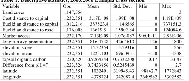
7. Descriptive statistics 7.1Cross Section
The descriptive statistics for the main variables are shown in Tables 1-3. The sample consists
of 1,232,351 one kilometer square cells that cover the entire area of Ethiopia.
The land cover classifications are disaggregated in Table 2. As shown, very little land is
assigned to urban area in the ESA dataset. This is expected because Ethiopia is a primarily rural
country. However, a contributing factor is also the fact that the smaller spatial extent of urban
area introduces higher classification error, leading to underestimation (Bicheron et al., 2008). For
this reason, my analysis focuses on the transition between vegetation (forest, shrubland, and
7.2Expressway
The descriptive statistics for land cover classification in 2009 and 2016 are shown in Table 4.
The sample consists of 487,551 140x140m cells in a 40-km buffer of the Addis Ababa-Adama
expressway. I have excluded any cells missing a land cover classification in one or both years
because of cloud cover, which obscures the image. Figure 5 shows the classified images of land
cover in both 2009 and 2016, with cloud cover a bigger problem in 2009 but still covering less
than 10 percent of the image.
As shown in the Table 4, the majority of land parcels in both 2009 and 2016 are devoted to
agriculture. However, a higher percentage of land is devoted to agriculture in 2009 versus 2016
(79 percent versus 68 percent). Approximately 66 percent of land devoted to non-agriculture in
2009 transitions to agriculture in 2016 while 15 percent of land that was agriculture in 2009
transitions to non-agriculture.
As acknowledged before, there is a degree of error in land cover classification. Since I cannot
physically inspect the land in order to verify and improve my classifications (ground-truthing),
the risk of error is increased. Additionally, the two images that I use (for 2009 and 2016) come
from different Landsat satellite images – Landsat 8 and Landsat 5, which may affect the
detection of surface reflectance and my classification. Therefore, I do not want to over-interpret
the fact that a decline in agriculture is observed between the two periods, since part this result
may be due to classification error. However, assuming that the error is random, I can still
accurately estimate the impact of my treatment variable (the expressway) on land use change
between agriculture and non-agriculture by looking at the spatial distribution of land cover
Descriptive statistics in Table 5 divide observations by their distance to the expressway
(within or outside a 20-km buffer). The table shows that land within the inner buffer of the
expressway is more likely to be agriculture in both 2009 and 2016, as compared to land outside
the inner buffer. Additionally, land closer to the expressway experiences a higher frequency of
transitions in both directions – from non-agriculture to agriculture and vice versa – during the
period of observation. I will explore these relationships further in my estimation, and offer
possible explanations.
8. Results and Discussion
The estimation of 𝛽 is based on equations (7) and (8). Using data on land cover for the whole
of Ethiopia in 2005/2006 and for the change in land cover in a 40-km buffer of the Addis
Ababa-Adama expressway after the expressway was built, between 2009 and 2016, I examine the effect
of distance to road/market on the probability of devoting a land parcel to agriculture.
8.1Cross Section
In my first estimation, I analyze a cross section of Ethiopia as a whole. I report the results
from a multinomial logit model in Tables 6-9, where the largest category (21% of observations),
Mosaic forest or shrubland (50-70%)/grassland (20-50%), is assigned as the base category. The
estimated coefficients in Table 6-9 represent the change in the log-odds of a given land cover
category relative to the base category for a one-unit change in the variable of interest, holding all
other variables constant. Of most interest are the coefficients on the distance variables (distance
Interpreting the results, we see a strong negative effect of an increase in distance to capital or
roads on the log-odds of urban area relative to the base category. Additionally, we see a smaller
negative effect of an increase in distance to capital or road on the log-odds agricultural land
classes relative to the base category. All estimations show a positive effect of market access on
the log-odds of urban area and agricultural land classes relative to the base category. Again, the
effect is stronger for urban areas.
Some categories with smaller numbers of observations shown outsized effects (for instance,
the largest effects in all models, either positive or negative, are on regularly flooded broadleaf
forest, for which there are only 50 observations). I expect that part of the reason for such a strong
effect on this category is because flooded broadleaf forest is heavily concentrated in regions
close to road networks and market for climactic reasons. Controls in the model for soil quality,
elevation, and latitude and longitude are not fully accounting for climactic factors. Thus, in
subsequent estimations, I add a factor variable for 68 administrative zones, in order to control for
unobserved characteristics of regions that will affect the prevalence of different land cover types.
In addition, I aggregate vegetation and agriculture categories, which reduces the problems posed
by small, localized land use categories.
Estimated marginal effects from the logit model are shown in Table 7. My main interest is in
the margins between different economic activities (idle land, agricultural activity, and urban
service or manufacturing). I focus on the margin between vegetation and agriculture because of
the small percentage of urban area in my sample (less than 0.01%) and the systematic
underestimation of urban area due to limitations of the classification methods used by the ESA
The results in Table 11 show statistically significant negative effects of distance to Addis
Ababa and positive effects of market access on the probability of devoting a land parcel to
agriculture across multiple specifications. The effect on log Euclidian distance to the Addis
Ababa shows that a one-percent increase in distance to the capital results in an 12-percent
decline in the probability of a land parcel being devoted to agriculture, on average. A one percent
increase in cost-distance to Addis Ababa leads to an average 15-percent decline in the probability
of agricultural land cover. Finally, a one-percent increase in market access is associated with an
average 5-percent increase in the probability of agricultural activity. Note that these are marginal
effects taken at the mean – as shown in Figure 8, the marginal effects vary depending on the
value of the explanatory variable (and tend to be largest near the mean). However, the signs of
the effects are the same and the effects remain statistically significant across all values. The
results are consistent with the theory developed by von Thünen, which predicts an increase in
agricultural land area at the margins when transportation costs decline.
The estimation results also show an insignificant positive effect of distance to road on
probability of agricultural land cover. This suggests that distance to a road matters less than the
travel costs to market along the road. Therefore, roads are not important in and of themselves,
but in how they reduce travel time to population centers. This result is notable because it is
contrary to the result from prior literature focused on the central and South America, which
found statistically significant negative effects of distance to road on the probability of agriculture
(Nelson and Hellerstein, 1997; Pfaff, 1999). A possible reason for the discrepancy is that
differences in the types of terrain and vegetation in Ethiopia versus central Mexico and the
Brazilian Amazon mean lower travel times in Ethiopia in the absence of roads, so roads make
non-agricultural economic activities nearby, such as residential or industrial uses that are not picked
up by the ESA classification system. It is out of the scope of this paper to test these hypotheses.
The interaction terms that include Euclidian distance to Addis Ababa and another
explanatory variable reveal how distance to the capital influences the magnitude of the reported
effects. The estimated results in Table 11 show a positive coefficient on the interaction between
log Euclidian distance to Addis Ababa and log cost-distance to Addis Ababa. So, at larger
distances from Addis Ababa, the effect from an increase in the cost of distance to market is
larger. Additionally, the coefficient on the interaction term between log market access and log
Euclidian distance to Addis is negative, showing that the effect of an increase in market access is
weaker at greater distances from the capital.
These results can be explained in several ways. First of all, when travel costs are higher, they
matter more to the profitability of farming. Therefore, for land parcels further away from Addis
Ababa (the largest market), travel costs may be more likely to make the difference between
whether agriculture is a profitable or unprofitable land use.
Additionally, closer to Addis Ababa, there are likely more alternative land uses to
agriculture, so that reductions in travel costs may promote expansion in economic activities other
than agriculture. This can be explained by the benefits of agglomeration described in Krugman
(1991): given larger existing manufacturing and service sectors close to Addis Ababa, the
benefits of economies of scale make areas near the capital more attractive for additional
manufacturing and service activities. Therefore, agriculture would tend to concentrate in more
rural areas where alternative economic activities are less viable.
Additionally, both the OLS and probit specifications that include the cost distance to Addis
of Euclidian distance on agricultural land use. This is opposite of the effect found when
Euclidian distance to Addis Ababa is included on its own. Therefore, separating the effect of
distance on increasing the cost of travel to the capital, land farther away from the Addis Ababa is
more likely agricultural. As with the direction of the coefficient on the interaction terms with
Euclidian distance to Addis Ababa, this result can be explained by the benefits of agglomeration
(Krugman, 1991) – a concentration of secondary and tertiary industries near the capital offer
more economic alternatives to agriculture that reduce likelihood of farming regardless of the
road network.
The coefficients on the control variables conform to expectation. Higher precipitation and
soil quality have positive and significant effects on the likelihood of a land parcel being devoted
to agriculture. Meanwhile, greater variation in elevation has a negative effect on the likelihood of
agricultural land cover.
8.2Expressway
In the second part, I estimate equation (8). Across all specifications, the results displayed in
Table 12 show a statistically significant negative average treatment effect on the treated. That is,
being in the treatment group (within an inner 20-km buffer of the expressway) is associated with
a lower probability of agricultural land cover. Additionally, across groups, land parcels with
higher soil quality and a higher neighboring concentration of agricultural activity are associated
with a lower probability of agricultural land cover in the second (treatment) period.
These results are counterintuitive, and contradict the initial theory. However, they are
consistent with the results from the cross-section that found positive, if insignificant, effects of
cross-section using only land parcels within the 40-km buffer of the Addis Ababa-Adama
expressway, I find that proximity to the capital and market access are negatively associated with
agriculture. These are opposite effects from when the model is estimated using the whole sample
of land parcels covering all of Ethiopia. This suggests that there is something unique about the
land surrounding the expressway. A discussion of possible reasons for the unexpected results,
including why land in near the expressway may respond differently to changes in transportation
costs than other land in Ethiopia, follows.
As mentioned in the analysis of the cross-section, one possible explanation for these results is
that agricultural land close to new roads (such as the expressway) is being transformed into
residential or industrial uses. Table 6 disaggregates percentage of agriculture by second-level
administrative region, and shows that the administrative region containing the core of Addis
Ababa is assigned to 28-percent agriculture in 2009 and 25-percent agriculture in 2016.
Therefore, likely some urban/industrial area is being captured in the non-agriculture category,
which would influence the results. Perhaps there is a higher benefit to proximity to roads for
urban/industrial land versus agricultural land and therefore agricultural land in close proximity to
roads is converted to other uses after road construction.
Additionally, the section of road and the surrounding land chosen for this analysis is unique
in several respects. The road is the only expressway in the country and connects the country’s
two largest cities, meaning that urban/industrial economic activity is more concentrated in this
part of the country than in more rural regions. As shown in the cross section, Euclidian distance
to Addis Ababa (the capital city which is included within the 40-km buffer of the expressway) is
associated with smaller positive effects of market access on probability of agriculture and
discussed, the estimating the logit model for the cross-section using only land parcels within a
40-km buffer of the expressway produces results with the opposite sign as when using the entire
sample. Therefore, the estimate treatment effect of road construction on agricultural land cover
may be unique to the area of analysis and not generally applicable across Ethiopia.
Finally, Euclidian distance to road may be a poor measure of transportation costs to market,
the true variable of interest. In the case of the expressway, distance to the road does not take into
account where are the entry points onto the expressway or changes that may have occurred over
the observation period in roads that connect to the expressway or other cities in the region. This
means that being within an inner buffer of the expressway may not be a good indicator of
treatment, if treatment is meant to measure a decline in transportation costs.
The results in Table 12 are only related to the change in the probability of agricultural land
cover, and do not take into account which transitions are taking place. There four possible (non)
transitions over the period: staying agriculture, staying non-agriculture, transitioning from
agriculture to non-agriculture, and transitioning from non-agriculture to agriculture. In Table 13,
I divide land parcels by their original classification in 2009, and look at how being in the
treatment or control group affects the probability of transition. As shown in the table, proximity
to the expressway results in a higher probability of transition both into and out of agriculture.
Therefore, treatment is associated with changes in land cover/use, but not solely in one direction
and overall out of agriculture.
Von Thünen’s theory of agricultural land use, the basis for this paper, can be applied to these
results. Von Thünen proposed that landholders maximize profits by allocating land to the most
cost-effective product, balancing land costs (higher nearer to market) and transportation costs
than grain because of faster spoiling. While Von Thünen’s theory assumes that agriculture is the
only economic activity outside of the city and that soil quality and climate are consistent
everywhere, this is evidently not true in our real-life sample of land surrounding the Addis
Ababa-Adama expressway. Therefore, a reduction in transportation costs changes the balance of
costs and benefits for different land uses – why we see transitions in land use near the
expressway –, but does not mean a transition towards agricultural activity in all cases.
The direction of the transition in land cover will depend on the relative value/cost of soil
quality, transportation, and other unobserved factors to different land uses. Thus, reducing
transportation costs can cause both an absolute increase in economic activity and a change in the
allocation of different types of economic activity across space, whether towards agriculture or
other uses. In this case, we see an increase in land cover transitions in proximity of the new
Addis Ababa-Adama expressway and an overall decline in agricultural activity.
Why do we see this result? Firstly, the estimation results may be due to the unique character
of land near the expressway. A re-analysis of the cross-section using only land parcels within
40-km of the expressway shows that proximity to Addis Ababa and market access are negatively
associated with agricultural land cover, the opposite effect found when using the full sample.
Likely the already highly urbanized nature of the land in this region impacts the response of
landholders to declining transportation costs. We may be seeing an increase in urban/industrial
activity after construction of the expressway that cannot be disaggregated from other
non-agricultural land cover types using the methodology in this paper. Additionally, it is possible that
my treatment variable is not well defined, and that proximity to the expressway is not a good
9. Conclusion
This study has shown that agriculture tends to be concentrated in regions with more access to
market. Using a cross-section of land cover in Ethiopia in 2005/2006, I show that agricultural
land use is more likely in areas with better access to market, after controlling for soil quality,
elevation, latitude and longitude, Euclidian distance to the capital, and administrative zone.
Additionally, I show that the effect of changes in cost distance is stronger for land further away
from the primate capital city (Addis Ababa). Unlike previous studies, I do not find a significant
effect on only distance to roads, ignoring market access.
Using panel data on land cover in a buffer of the Addis Ababa-Adama expressway, I show
that proximity to the expressway increases the likelihood of transitions both into and out of
agriculture. Additionally, I found a negative average treatment effect on land parcels within an
inner buffer of the expressway during the treatment period (after the construction of the
expressway). Proximity to the expressway is therefore associated with a decline in agricultural
activity compared to with land parcels farther away from the new expressway. A re-analysis of
the estimation from the cross-section using only the land parcels in within 40-km of the future
expressway shows a negative effect of proximity to Addis Ababa and market access on
probability of agricultural land cover. This confirming that a decline in transportation costs in
this part of the country does not increase agricultural land cover on average.
The results indicate that reducing transportation costs/increasing market access can play an
important role in spurring economic activity, including an expansion in agricultural land use.
However, the effect is not the same everywhere: reducing travel costs to more rural areas – those
farther away from the densely-populated capital region in Ethiopia – has a greater effect on
means to reduce travel costs, I find that proximity to them, without taking into account other
measures of market access, is in fact associated with a decline in agricultural land use. This
effect is perhaps because of increases in urban/industrial activities near roads, or because of other
unobserved factors.
This study adds to the literature by using a new measure of market access that takes into
account cost-distance to all major markets, and by looking at a wider geographic area (the whole
of Ethiopia) than previous studies. I demonstrate the feasibility of using newly-available
satellite-derived land cover data, such as the European Space Agency dataset, to evaluate
changes in the spatial allocation of economic activity. Additionally, I show that reducing
transportation costs through road construction can be an effective way to grow Ethiopia’s
economy by spurring agricultural activity. However, effects of road construction on agricultural
activity may not be the same across the entire country. Additionally, satellite data is most useful
for analyzing changes in agricultural land cover, since urban/industrial land cover is difficult to
classify and therefore typically under-estimated.
While the focus of this study is on Ethiopia, the same empirical results could be present in
other primarily rural countries experiencing a significant road network expansion. An area of
further research would be to compare the economic benefits of increasing agricultural and other
types of economic activities with the costs of road construction.
Limitations of this study include the systematic underestimation of urban area classified from
satellite imagery and lack of data due to the time-intensive nature of land cover classification
when no pre-classified imagery is available. Future studies should enhance the accuracy of
future studies should compare land cover change after the construction of roads in both urban
and rural areas, in order to determine if different responses occur.
10.References Literature:
Ai, C., & Norton, E.C. (2003). Interaction terms in logit and probit models. Economic Letters,
30, 123-129.
Allen, T. & Arkolakis, C. (2014). Trade and the topography of the spatial economy. The
Quarterly Journal of Economics, 129(3), 1085-1139.
Alonso, W. (1964). Location and land use: Toward a general theory of land rent. Cambridge:
Harvard University Press.
Baum-Snow, N. (2007). Do highways cause suburbanization? The Quarterly Journal of
Economics, 122(2), 775-805.
Bicheron P., Defourny P., Brockmann C., Schouten L., Vancutsem C., Huc M., Bontemps S., Leroy M., Achard F., Herold M., Ranera F., Arino O. (2008). Globcover products description and validation report. Medias France, Toulouse, France. Available online at http://due.esrin.esa.int/files/GLOBCOVER_Products_Description_Validation_Report_I2.1 .1.pdf
Chomitz, K.M. & Gray, D.A. (1996). Land use, and deforestation: A spatial model applied to
Belize. The World Bank Economic Review, 10(3), 487-512.
Dercon, 2004. Growth and shocks: evidence from rural Ethiopia. Journal of Development
Economics, 74(2), 309-329
Dercon, S., Hoddinott, J., & Woldehanna, T. (2012). Growth and chronic poverty: Evidence
from rural communities in Ethiopia. Journal of Development Studies, 48(2), 238–253.
Dercon, S. & Hill, R.V. (2009), Growth from agriculture in Ethiopia: identifying key constraints. Retrieved from: http://users.ox.ac.uk/~econstd/Ethiopia%20paper%203_v5.pdf
Donaldson, D. (in press). Railroads of the Raj: Estimating the Impact of Transportation Infrastructure. American Economic Association.
Donaldson, D., & Hornbeck, R. (2016). Railroads and American economic growth: A “market
Dorosh, P., & Thurlow, J. (2013). Can cities or towns drive African development? Economywide
analysis for Ethiopia and Uganda. World Development, 63, 113-123.
Eaton, J. & Kortum, S. (2002). Technology, geography, and trade. Econometrica, 70(5),
1741-1779.
Embassy of Ethiopia in Beligum (2014). Ethiopia’s first expressway nears completion. Retrieved
from: http://www.ethiopianembassy.be/en/2014/04/14/ethiopias-first-expressway-nears-completion/
Faber, B. (2014). Trade integration, market size, and industrialization: Evidence from China’s
national trunk highway system. Review of Economic Studies, 81, 1046-1070.
Federal Democratic Republic of Ethiopia. (2015). The Second Growth and Transportation Plan.
Addis Ababa: National Planning Commission.
Fenta, K. (2014). Industry and industrialization in Ethiopia: Policy dynamics and spatial
distributions. European Journal of Business and Management, 6(34), 326-344.
Fourie, E. (2015) ‘China’s example for Meles' Ethiopia: when development “models” land.’ The
Journal of Modern African Studies, 53(3), pp. 289–316.
Glaeser, E.L. (2008). Cities, agglomeration and spatial equilibrium. New York: Oxford
University Press.
Fujita, M., Krugman, P., & Venables, A.J. (1999). The spatial economy. Cambridge: MIT Press.
Krugman, P. (1991). Increasing returns and economic geography. Journal of Political Economy,
99(3), 483-499.
Lavers, Tom. (2012) ‘Land grab’ as development strategy? The political economy of agricultural
investment in Ethiopia. The Journal of Peasant Studies, 39(1), 105-132.
Li, B. (2011) The multinomial logit model revisited: A semi-parametric approach in discrete
choice analysis. Transportation Research Part B: Methodological, 45(3), 461-473
Mills, E.S. (1972). Urban economics. Glenview, Illinois: Scott Foresman.
Muth, R.F. (1969). Cities and housing. Chicago: University of Chicago Press.
Natchergaele, F., van Velthuizen, H., Verelst, L., & Wilberg, D. Harmonized World Soil
Database (version 1.2). Rome, Italy: FAO, and Austria: IIASA.
Nelson, G.C. & Hellerstein, D. (1997) Do roads cause deforestation? Using satellite imagines in
econometric analysis of land use. American Journal of Agricultural Economics, 79(1),
Pfaff, A.S.P. (1999). What drives deforestation in the Brazilian amazon? Evidence from satellite
and socioeconomic data. Journal of Environmental Economics and Management, 37, 26-43
Puhani, P.A. (2012). The treatnment effect, the cross difference, and the interaction term in
non-linear “difference-in-difference” models, Economics Letters, 115(1), 85-87.
Roberts, M., Deichmann, U., Fingleton, B. & Shi, T. (2012). Evaluating China’s road to
prosperity: A new economic geography approach. Regional Science and Urban
Economics, 42, 580-594.
Russel, C. (2014). Global land cover mapping: A review and uncertainty analysis. Journal of
Remote Sensing, 6(12), 12070-12093
Shiferaw, A., soderbom, M., Eyerusalem, S., & Alemu, G. (2015). Road infrastructure and
enterprise dynamics in Ethiopia. Journal of Development Studies, 51(11), 1541-1558.
USDA Foreign Agriculture Service (2016). Ethiopia’s agriculture imports continue growing (Report No. ET1634). Retrieved from: https://www.fas.usda.gov/data/ethiopia-ethiopia-s-ag-imports-continue-growing
Worku, I. (2011). Road sector development and economic growth in Ethiopia. Addis Ababa:
Ethiopian Development Research Institute.
World Bank. (2016). Ethiopia’s great run: The growth acceleration and how to pace it.
Washington, DC: World Bank Group.
Table 1: Descriptive statistics, 2005/2006 Ethiopia cross section
Variable Obs Mean Std. Dev. Min Max
Land cover 1,147,556 1 3
Cost distance to capital 1,232,351 3.17E+08 1.99E+08 0 1.19E+09 Euclidian distance to capital 1,012,216 387823.8 146565 0 737151.3 Euclidian distance to road 1,176,008 13619.51 15902.84 0 124084.6 Market access 1,232,170 7.13E-09 3.07e-087 9.60E-11 2.93E-06 long run avg precipitation 1,232,351 816.4738 426.4613 126 1800 elevation stdev 1,232,351 14.32354 15.59316 0 256 elevation mean 1,232,351 1223.103 696.0951 -150 4338 topsoil organic carbon 1,220,520 0.9264244 0.7332208 0.17 33.87 Difference from pH =7 1,223,524 0.7433856 0.5245469 0 2.7 latitude 1,232,351 1032491 319945.43 98842.7 1772843 longitude 1,232,351 4378724 342087.4 3649582 5302582
Land Cover Frequency Percent
Rainfed croplands 30,162 2.45
Mosaic cropland (50-70%)/vegetation (20-50%) 209,492 17 Mosaic vegetation (50-70%)/cropland (20-50%) 181,674 14.74 Closed to open >15% broadleaved evergreen or semi-deciduous forest (>5m) 13,673 1.11 Open (15-40%) broadleaved deciduous for 57,424 4.66 Mosaic forest or shrubland (50-70%)/grassland (20-50%) 258,933 21.01 Mosaic grassland (50-70%)/forest or shrubland (20-50%) 3,074 0.25 Closed to open (>15%) shrubland (<5m) 172,517 14 Closed to open (>15%) herbaceous vegetation 67,332 5.46 Sparse (<15%) vegetation 153,220 12.43 Closed to open (>15%) broadleaved forest regularly flooded 50 0 Closed to open (>15%) grassland or woody vegetation on regularly flooded or
waterlogged soil 2,503 0.2
Urban >50% 137 0.01
Bare areas 74,429 6.04
Water bodies 7,731 0.63
Land Cover Frequency Percent Vegetation 890,464 77.6 Cropland 256,951 22.39 Urban Area 141 0.01 1,147,556 100
Variable Observations Mean Min Max Agriculture in 2009 487,551 0.7852 0 1 Agriculture in 2016 487,551 0.6767 0 1 If agriculture in 2009 157,606 0.6566 0 1 If non-agriculture in 2009 329,945 0.1534 0 1 Agriculture concentration 863,368 0.6873 0 1 Ideal topsoil pH 975,102 0.8094 0 1 Within 20km of expressway 975,102 0.389 0 1