2019_Whitley.pdf

(1)

Multi-Component Diffusion Study and Stability

Analysis

Victoria Whitley

April 8, 2019

Abstract

(2)

1 Introduction

Multi-component diffusive convection, where the flow density depends on more than two components, has applications in many natural fields such as oceanography, geo-physics, environmental engineering, and astrophysics [9],[14]. In the standard con-vection problem, instabilities are driven by density differences between the upper and lower planes bounding the fluid [9]. In thermal convection, a fluid with a higher temperature will be less dense, allowing the parcel of fluid to rise, while colder fluid will fall because it is denser than its surroundings. If the fluid layer in question also has some concentration of another substance dissolved within, there are two destabilizing sources. The most common naturally produced scenario, thermoha-line convection, involves a temperature field and sodium chloride [3]. When there are two effects, with competing stabilizing and destabilizing forces, the convection phenomenon is called double diffusive convection. In double diffusive flows, the two components often have very different molecular diffusivities, which operate on dif-ferent time scales [14]. These differences induce interesting flow phenomena such as salt-fingers and oscillating convection cells within the fluid plane. By introducing a third component, the competing behaviors give rise to many combinations of stabi-lizing and destabistabi-lizing phenomena. Applications of this research include modeling geothermal reservoirs, harnessing the sun’s energy through solar ponds, and under-standing pollution transport [9].

The fingering and oscillation effects usually associated with double diffusion have been recorded in many recent experiments involving the density stratification of corn syrup. To understand if this behavior is connected to multi-component convec-tion or if it is a separate phenomenon, we ran several trials using sharply stratified corn syrup and water mixtures. By analyzing the behavior of these experiments and comparing the results with a stability analysis for multi-component convection, we can better understand the processes at work in these situations.

2 Background

(4)

in an ocean with its upper end in warm, salty water and its lower end in denser, cooler, and fresher water. By pumping fluid from below, through the pipe, the water inside quickly reaches the same temperature as the surrounding ocean outside of the pipe, but this water remains fresh because the salt cannot permeate the pipe walls. This fresh fluid is less dense than the surround water, allowing the water to flow up the pipe. Water from below would continue to move up the pipe until the salinity gradient is gone [3].

Figure 1: A field of salt fingers formed by setting up a stable temperature gradient and pouring a salt and fluorescein solution on top [3], [4].

(5)

and continues to rise. Conversely, a fluid parcel that drops by ∇z, quickly becomes heavier than the surrounding fluid as it loses heat, and it continues to sink [4]. These parcels that quickly sink or rise create long and narrow convection cells, called salt fingers. Figure (1) presents a field of salt fingers contrasted with the surrounding fluid by using fluorescein dye [3]. Stern predicted the scale of these fingers using a linear instability calculation [7].

Figure 2: A series of convecting layers and ’diffusive’ interfaces, formed by heating a gradient ofK2CO3 solution from below [3].

Stern also found through his stability analysis that the opposite situation, with cold, fresh water over warm, salty water, corresponds to oscillatory instability [3]. Considering the same initial perturbation, the lighter fluid parcel moved up by ∇z

(6)

the Rayleigh-Bernard problem [4]. When some critical Rayleigh number is reached, it becomes unstable and a second convecting layer forms above the first [3]. In many cases, the fluid forms several distinct mixed layers as seen in Turner and Stommel’s investigations [3]. Such convecting layers can be seen in Figure (2), where a K2CO3 solution was heated from below.

Veronis [12],[13] realized that the layers and interfaces first studied by Turner and Stommel (1964) could only be explained theoretically by a nonlinear theory [3]. In an extended Rayleigh-Benard problem, Veronis studied the two-dimensional behav-ior of fluid bounded by two horizontal planes, heated and salted from below [3]. By solving the partial differential equations for conservation of momentum, heat, and salt, researchers found two different solutions, a steady, direct case and an oscilla-tory case, corresponding to the observed phenomenon. The stability analysis and experimental results revealed that, under certain conditions and perturbations, the resulting destabilization can create movement and density transfers in ways that are very different from the one-component case.

3 Diffusion Experiments

To study the impact of multi-component or double diffusion on stratified solutions, we conducted a series of experiments, varying the densities of the fluid and the salt involved. The initial experiments mixed Karo corn syrup with water to create ”fresh” fluids varying in densities from 1.20022 to 1.12013 g/cm3. These corresponded to specified ratios of water( ρ ≈ 1g/cm3_{) and corn syrup (}_ρ _≈ ₁_.₃₆_g/cm3_{), From 4} parts water and 2 parts corn syrup (4:2) up to five parts corn syrup (4:5). As the phenomena has been observed more often in viscous Karo experiments and less in water, by taking a range of densities we could estimate a critical density threshold for these phenomena. These solutions were created by adding water to the corn syrup using a magnetic stirrer, until the densities were within 0.0005g/cm3 of the specified amount.

Each density mixture was then split into two 500 mL containers for the stratification. A calculated amount of salt was added to the bottom layer to increase the density by 0.004 g/cm3_, _{as well as two drops of dye, which created a visual difference between} the layers. The bottom layer was mixed for at least twenty minutes, again, using the magnetic stirrer.

(7)

by “floating” the lighter layer on top to maintain an initially sharp stratification. This is done by floating a sponge supported by a highly buoyant material such as styrofoam on the surface of the bottom layer. Filtering the top layer through the sponge disperses the lighter fluid over a broad area, minimizing the mixing between layers. As more fluid is added, the foam allows the sponge to rise with the top layer, allowing the top layer to increase above a sharp stratification.

Once stratified, the four solutions, ranging from the densest at approximately 1.20022

g/cm3 _{to the least dense at 1.12013} _g/cm3 _{were covered with plastic wrap and left} to naturally diffuse. The solutions were left at room temperature, susceptible to any fluctuations. Interval shots were taken with a Nikon D3 camera to visually record the diffusion process. Density, conductivity, and viscosity measurements were taken from the top and bottom layer, 5 mm below the surface and 5 mm above the bottom, be-fore and after the experiment. In later experiments, post-experiment measurements of density, conductivity, and viscosity were also taken at the initial point of stratifi-cation, 45 mm from the bottom. In the final experiments, continuous temperature measurements in the two density extremes were recorded using thermistors placed 10mm below and above the initial point of stratification. For visual reference, see Appendix B for all measured values.

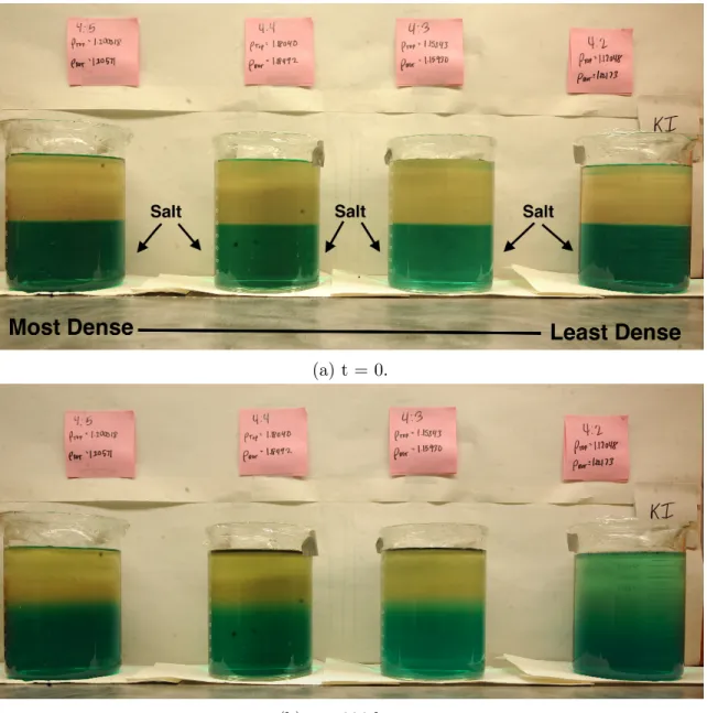
Four salts were used to increase the density within the solution, NaCl, NaI, KCl, and KI. The combination of salts allowed us to look at the differences between a Chloride and Iodide base when combined with Sodium and Potassium. The length of time each experiment lasted varied slightly for each salt because of the longer time it takes some salts to diffuse over others. The experiments were ended when the dye had visually diffused over most of the solution. One such experiment can be seen in Figure (3).

Since NaCl is the substance behind thermohaline convection and previous exper-iments by Valchar [11] had recorded the fingering and oscillatory destabilizations with NaCl, more extended experiments were done using this salt. One “zoomed in” experiment looked at a set of four densities ranging between the two most dense so-lutions that were used in all of the experiments, 1.20022g/cm3 _{and 1.19406} _g/cm3_. Using the water to corn syrup ratio language described earlier, these solutions were

(8)

(a) t = 0.

(b) t = 306 hours.

(9)

4 Results

4.1 Potassium Iodide (KI)

From a visual analysis of the Potassium Chloride or KI experiment, it is immediately clear that no instabilities occur within the given density range. The KI solutions showed no fingering or oscillatory behavior. The least dense solution diffused the fastest. The denser the solution, the longer the dye took to diffuse. Such a correlation can be seen in Figure (3b), where the dye in the least dense (far right) has diffused completely, but the densest has barely changed from the initial stratification.

Comparing the measurements taken before and after the experiment, the density and viscosity changed very little in the top or the bottom for KI. It is clear that some kind of diffusion occurred, though, due to the change in conductivity. The conductivity reading for the top of all four solutions doubled over the course of the experiment, significantly reducing the difference between the top and bottom. Since electrical conductivity is largely influenced by the salt concentration within the solution, this change implies that the salt diffused throughout the mixture over time as one would expect.

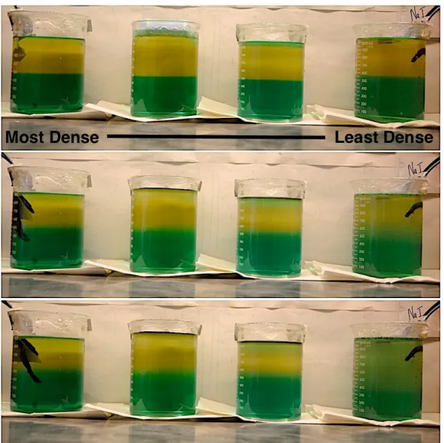
4.2 Sodium Iodide (NaI)

Sodium Iodide or NaI also exhibited no visible signs of oscillatory or fingering behav-ior. Similar to KI, the most dense solution diffused the slowest, with speed inversely related to density, as one would expect in a singular diffusion environment. Figure (4) shows how the dye diffused evenly in this experiment, with images taken at the beginning, middle, and end.

(10)

(11)

Temperature was also measured using four thermistors placed in the two extremes of the densities observed, 10 mm above and below the initial stratification line. Within the first twenty hours there was an initial increase of 1.5 degrees, measured in both the top and the bottom of (4:5) and in the top of (4:2). The bottom of (4:2) measured an initial 1 degree increase. After that, the solutions remained relatively constant, with a small increase of about 0.5 degrees over time in all measured points. This increase did not correspond to any specific visual changes in the dye.

4.3 Potassium Chloride (KCl)

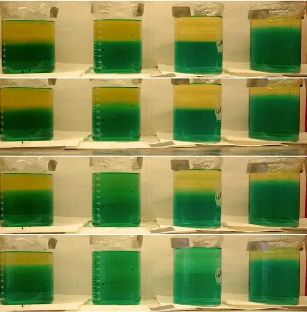
Within minutes of stratifying with Potassium Chloride, or KCl, the denser solutions began to show signs of fingering. First in the most dense (ρ4:5T op = 1.20005g/cm3) and soon in the next solution (ρ4:4T op = 1.18077g/cm

3_{). In the most dense (4:5)} solution, the fingering effect also involved very short oscillations. This caused the dye to diffuse in very visible spurts or steps. After forty hours, the dye hit some kind of barrier halfway up the top part of the stratification and did not diffuse any farther, even though the experiment was left running for another twenty-six hours. In contrast, the second most dense (4:4) quickly formed long fingers which doubled back into oscillation halfway up, overtaking the rest of the solution in the next oscillation or step. This change in the size of the oscillatory layers allowed the dye to be completely uniform throughout within only eleven hours. The next solution (4:3), did show signs a minimal fingering, but mostly looked to diffuse at a normal rate. Within twenty-four hours the dye in the third most dense had diffused uniformly. The results of the least dense solution (4:2) were contaminated due to stratification issues, causing very little convection to take place at all. The final levels of the dye and some of the fingering effect in (4:4) can be seen in Figure (5), where the left most solution is the densest.

As measured, the density in the top and bottom did not change at all. Viscosity in the top increased by 1 mPa*s in the middle two solutions, but the most and least dense saw no change in the top or bottom. The conductivity increased by 500

(12)

(13)

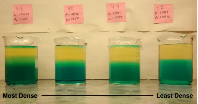
4.4 Sodium Chloride (NaCl)

Figure 6: Fingering effect in NaCl and dye stratified diffusion

As the source of the original observation of this phenomenon, the majority of the experiments were focused on Sodium Chloride’s impact on convection. With two trials using the same density range as the other salts, two looking in depth at the two densest values in the original range, and one looking at denser solutions than the original four, we were able to get a better idea of what factors impact the oscillations and fingering observed.

(14)

though present in the middle two solutions, were smaller, creating the slower steps up the beaker as layers formed. In both cases, after forty-eight hours the dye reached a point it could go past and did not diffuse in the upper third of the beaker. The least dense solution exhibited no oscillatory or fingering behavior. This trial was purely a visual trial and no measurements were taken at the end of the experiment to make comparisons.

Figure 7: Oscillatory Effect in NaCl Stratified Solution

(15)

completely uniform. This allowed the dye in the denser solution to diffuse within fourteen hours, before the less dense ones. By looking at the conductivity measure-ments in the top and bottom, it is clear that the salt also diffused upwards, as the conductivity decreased in the bottom and increased in the top. Over the course of the experiment, the bottom of the (4:4) solution became denser by 0.005g/cm3

and more viscous by 1.17mPa*s, which was the largest increase in both density and viscosity in this experiment. The top also showed increases in viscosity and density. The next solution (4:3) was observed to have some layering creating by oscillations. Though there was very little change in the conductivity, in the conductivity profile, the maximum amount was actually about 30mm from the bottom, still below original stratification line. There was very little change in density, but viscosity increased in both the top and the bottom, where the top actually surpassed the viscosity in the bottom. The least dense solution (4:2) diffused evenly throughout the experiment with no noticeable effects present. The density in the bottom of this solution ex-perienced the largest increase, going from 1.12436g/cm3 _{to 1.13055}_g/cm3_{, while the} density in the top changed very little. The solution became equally more viscous in the top and the bottom, possibly stemming from some form of evaporation. The conductivity measurements show that the salt did diffuse some, but not enough to shorten the difference between the top and bottom by much. Temperature measure-ments were taken in the least (4:2) and most dense (4:5) solutions, 10 mm above and below the interface. In the least dense, the bottom temperature increased by 1.5 degrees in the first ten hours. The warmer top solution only increased by 1 degree within that time frame. The temperature difference remain stable after that point for the rest of the experiment. In the most dense experiment, the bottom layer was actually warmer than the top, creating an unstable gradient. Unfortunately, the when the thermistors separated from the side, the two temperatures quickly reached an equilibrium for the rest of the experiment, and we are unable to tell how the temperature in the bottom layer changed.

(16)

vis-cous over time while the bottom changed very little. These solutions did experience some diffusion, as all showed decreases in conductivity over time in the bottom.

In the second zoomed experiment, the most dense, corresponding to the regular (4:5), exhibited some fingering and the only oscillatory behavior detected was based on the mixed layers of dye that moved up in steps and spurts rather than a steady diffusion. Yet, the conductivity in this solution did not change significantly. The top grew less dense and much less viscous than the start, a decrease of 1.42 mPa*s. The loss of density and viscosity in the top suggests that the salt did not diffuse, but the lighter material rose to the top a one would see in a standard convection problem. The mid-dle two experiments that fell between the usual (4:4) and (4:5) exhibited minimal fingering and never fully diffused over the course of the experiment. Their top layers also became considerably less viscous and less dense. The only difference, seen in (4 : 41₃), was that the bottom density decreased on par with the top, maintaining the change in density over time within this solution. Neither solution showed signif-icant change in conductivity, suggesting that the salt did not diffuse over the course of the experiment. The least dense for this experiment corresponds to the second most dense in the other experiments, that of an equal ratio of water and corn syrup (4:4). In this case, the solution (ρT op4:4 = 1.17987) did not exhibit any fingering, but

immediately started large oscillations, allowing for uniform dye within twenty-four hours. In this solution, you see a similar change in viscosity as in the other solutions, but unlike the others, the density actually increased in both the top and the bottom. The conductivity also increased in the top and decreased in the bottom, showing a good amount of the salt diffused upwards. We were also able to take temperature measurements in this trial, straddling the interface in the least and most dense, (4:4) and (4:5) respectively. In (4:4), there was an intial 0.5 degree difference in the two layers, with warmer fluid on top. Within the first 20 hours, both layers grew warmer by half of a degree, but in the next ten hours the solutions stabilized again, dropping back down to the initial values for the rest of the experiment. In (4:5), the top was only 0.3 degrees warmer than the bottom. This difference remained steady as the temperature increased then decreased by the same 1 degree amount, before reaching a steady temperature.

Finally, we looked at denser, more viscous solutions than the original experiments ranging from (ρ_4:51

2T op = 1.20901) to (ρ4:4

3

(17)

solu-tions, diffused farther, about halfway up the top stratification layer, but then they also stopped. Yet, the conductivity profiles show a smooth transition from the top to the bottom, indicating that the salt diffused when the dye did not. The bottom density and viscosity did not change much, but the top grew considerably less dense and less viscous over time. Looking at temperature measurements in (4 : 51₂), the top started off as only .2 degrees warmer than the bottom, but in the first twenty hours, the temperature in the top increased by 1.5 degrees while the bottom increased by only 1 degree, these values remained stable for the rest of the experiment. In (4 : 43₄), the bottom was 0.5 degrees warmer than the top, and the solution maintained this difference during the initial 1.5 degree increase and during the stability afterwards.

5 Theory

5.1 Initial Conditions and Governing Equations

To understand the multi-component phenomenon, we must look at the stability of the diffusion problem. Creating a theoretical framework from which we can see if and when these fingering and oscillation behaviors occur will allow us to conjecture on the correlation between the experimental results and the destabilizing forces at play.

Consider a porous material held in a confined horizontal layer. The bottom layer is at z’ = 0 and the top is at z’ = H. The temperature is specified at both boundaries of the solution and the normal component of the velocity, W, is zero. The composition of salt and dye are specified at both boundaries.

T_H0 =TH, CSa0 =C 0

SaH, C 0 d=C

0

dH, W 0

= 0, at z0 =H (1)

T₀0 =T0, CSa0 =C 0

Sa0, C

0 d=C

0

d0, W

0

= 0, at z0 = 0 (2)

(18)

ρ0cp[

∂T0 ∂t0 +U

0_{· ∇}

T0] =k∇2_T0

(3)

∂C_Sa0 ∂t0 +U

0_{· ∇}

C_Sa0 =DSa∇2CSa0 (4)

∂C_d0 ∂t0 +U

0 _{· ∇}

C_d0 =Dd∇2Cd0 (5)

U0 =−Π0

µ ∇p

0

+ρ0(T0, C_Sa0 , C_d0)gkˆ (6)

∇ ·U0 = 0. (7)

The density of the fluid in the gravity term is given by

ρ0(T0, C_Sa0 , C_d0) =ρ0[1−αSa(CSa0 −CSa0)−αd(C

0

d−Cd0) +β(T

0 ₋

T0)]. (8)

The composition dependence of the density is only included in the gravity term, and all other appearances are assumed to be the reference density,ρ0, at the position z’ = 0. Additionally, cp is the specific heat per mass, k is the thermal conductivity, and Di is the solute diffusivity for substance i. Π0 is the permeability of the porous medium,µthe fluid viscosity,g is the gravitational acceleration, ˆkthe unit vector in the vertical direction, and αi and β are solutal and thermal expansion coefficients. Due to the sign convention chosen in the density equation, if α >0 and β >0 the density increases with concentration and decreases with temperature

5.2 Non-dimensional Equations

Now, normalizing the above equations, lengths are scaled with the layer thickness

H, time with H_κ2, and velocity with _Hκ (where κ = _ρk

0cp is the thermal diffusivity). We can also make temperature dimensionless withT = T0−TH

T0−TH, such that ifT 0 ₌_T

H, then T = 0, and if T0 = T0, then T = 1. Similarly for concentration i = Sa, d

Ci =

C_i0−C_iH Ci0−CiH.

Dimensionless pressure is given by

p= Π0

κµp

0

(9)

(19)

∂T

∂t +U · ∇T =∇

2_T ₍₁₀₎

∂CSa

∂t +U · ∇CSa=

1

LeSa ∇2_C

Sa (11)

∂Cd

∂t +U · ∇Cd=

1

Led

∇2Cd (12)

∇ ·U = 0. (13)

U =−∇p+ [−G+RaT(T −1)−RaCSa(CSa−1)−RaCd(Cd−1)]ˆk (14)

subject to the boundary conditions:

T = 0, CSa = 0, Cd= 0, W = 0, at z= 1 (15)

T = 1, CSa = 1, Cd= 1, W = 0, at z= 0 (16)

The dimensionless parameters in the above equations are

G= ρ0gHΠ0

κµ , RaT =

β(T0−TH)ρ0gHΠ0

κµ , RaCi =

αi(Ci0−CiH)ρ0gHΠ0

κµ , Lei =

κ Di,

for i = Sa and d.

The Lewis numberLei represents the ratio of thermal (κ) to solutal diffusivity (Di), and is typically much greater than one. G is a dimensionless parameter representing the ratio of hydrostatic pressure ρ0gH to the viscous pressure scale and will only influence the base state pressure. The Rayleigh numbers, RaCi represent solutal buoyancy in the different solutes and RaT represents thermal buoyancy. Assuming positive α and β, one would expect destabilizing scenarios when RaT > 0, corre-sponding to warm fluid under colder fluid (T0 > TH), and RaCi <0, corresponding to fresh fluid near the bottom layer and salty, dyed or more sugary fluid at the top (C0 < CH).

5.3 Steady Base State

(20)

U =0, TB(z) = 1−z, CSaB = 1−z, CdB = 1−z. (17) The pressure in the base state is also only a function of z, and dpB

dz =−G−RaTz+

RaCSaz+RaCdz. In the dimensional form the density gradient has the form

dρB

dz =ρ0

−αSa(CSa0 −CSaH)−αd(Cd0 −CdH) +β(T0−TH)

. (18)

Static stability can be defines as when density decreases with vertical position (dρB dz < 0), ie. heavier fluid over light fluid. The combination of thermal and solutal fields determine this base state density gradient. A specific base state is statically stable with respect to temperature if β(T0−TH) < 0, meaning, if taken alone, the tem-perature field would indicate stability if T0 < TH. Similarly, a specific base state is statically stable with respect to the concentration of a solute ifα(C0−CH)>0. In this system there are 14 basic combinations of the solutal effects.

1. All solutal fields are stabilizing ( warm, fresh fluid over cold, salty, dyed fluid )

2. All solutal fields are destabilizing ( cold, salty, dyed fluid over warm fresh fluid)

3. Some combination of stabilizing and destabilizing agents

For (1) and (2), all agents are promoting the same outcome, making the stability prediction simple, but case (3) lead to competing agendas and an unknown stability outcome, studied in the following section.

5.4 Disturbance Equations

Consider two-dimensional perturbations to the base state solution of the form

T =TB(z) + ˜T(x, z, t), (19)

CSa =CSaB(z) + ˜CSa(x, z, t), (20)

Cd=CdB(z) + ˜Cd(x, z, t), (21)

U =0+ ˜U(x, z, t), (22)

(21)

where ˜U = ( ˜U ,W˜).

Substituting these into the disturbance equations, consider for concentrations i = Sa and d

∇Ci =∇(CiB + ˜Ci)

=∇(1−z+ ˜Ci)

=∂ ˜

Ci

∂x , ∂C˜i

∂z −1

Then,

U · ∇Ci =

_˜

U ,W˜·∂C˜i

∂x , ∂C˜i

∂z −1

= ˜U · ∇Ci−W˜

Finally, since ∇2_C

iB = 0,

∇2_C

i =∇2C˜i

Therefore,

∂Ci

∂t +U· ∇Ci =

1

Lei ∇2_C

n

becomes

∂C˜i

∂t + ˜U · ∇Ci−

˜

W = 1

Lei ∇2C˜i.

For temperature,

∇T =∇(TB+ ˜T)

=∇(1−z+ ˜T)

=∂ ˜

T ∂x,

∂T˜ ∂z −1

(22)

Then,

U · ∇T =U ,˜ W˜·∂T˜

∂x, ∂T˜

∂z −1

= ˜U · ∇T −W˜

Therefore,

∂T

∂t +U · ∇T =∇

2_T

becomes

∂T˜

∂t + ˜U · ∇T −

˜

W =∇2_{T .}_˜

Since dpB

dz =−G−RaTz+RaCSaz+RaCdz,

U =−∇p+−G+RaT(T −1)−RaCSa(CSa−1)−RaCd(Cd−1)

_ˆ

k

=−∇p˜+ [−dpB

dz + (−G+RaT( ˜T −z)−RaCSa( ˜CSa−z)−RaCd( ˜Cd−z))

_ˆ

k

=−∇p˜+

RaTT˜−RaCSaC˜Sa−RaCdC˜d

_ˆ

k

So, the perturbations satisfy the equations

∂T˜

∂t + ˜U· ∇T −

˜

W =∇2_{T ,}_˜ ₍₂₄₎

∂C˜Sa

∂t + ˜U · ∇CSa−W˜ =

1

LeSa ∇2_C_˜

Sa, (25)

∂C˜d

∂t + ˜U· ∇Cd−

˜

W = 1

Led

∇2C˜d, (26)

−∇p˜+RaTT˜−RaCSaC˜Sa−RaCdC˜d

_ˆ

k= ˜U, (27)

∇ ·U˜ = 0. (28)

(23)

curl twice and use the Laplacian relationship, ∇ × ∇ ×U˜ =∇(∇ ·U˜)− ∇2_U˜_{. Due} to equation (28), we have∇ × ∇ ×U˜ =−∇2_U_˜_.

Then,

−∇2_U ₌_{∇ × ∇ ×}

− ∇p˜+RaTT˜−RaCSaC˜Sa−RaCdC˜d

_ˆ

k

=∇ × ∇ ×

− ∂p˜

∂x,− ∂p˜

∂z +RaT

˜

T −RaCSaC˜Sa−RaCdC˜d

=∇ × ∂ ∂z

− ∂p˜

∂x

− ∂

∂x

−∂p˜

∂z +RaT

˜

T −RaCSaC˜Sa−RaCdC˜d

ˆ j =∇ × − ∂

2_p_˜

∂x∂z + ∂2p˜

∂x∂z −RaT ∂T˜

∂x +RaCSa

∂C˜Sa

∂x +RaCd

∂C˜d

∂x ˆ j = RaT

∂2_T_˜

∂x∂z −RaCSa

∂2_C_˜ Sa

∂x∂z −RaCd

∂2_C_˜ d

∂x∂z,

−RaT

∂2_T˜

∂x2 +RaCSa

∂2_C˜ Sa

∂x2 +RaCd

∂2_C˜ d

∂x2

.

So

∇2U˜ =−RaT

∂2_T_˜

∂x∂z +RaCSa

∂2_C_˜ Sa

∂x∂z +RaCd

∂2_C_˜ d

∂x∂z (29)

∇2_W_˜ ₌_Ra T

∂2_T_˜

∂x2 −RaCSa

∂2_C_˜ Sa

∂x2 −RaCd

∂2_C_˜ d

∂x2 . (30)

(24)

∂T˜ ∂t −

˜

W =∇2_T_˜ ₍₃₁₎

∂C˜Sa

∂t −

˜

W = 1

LeSa ∇2_C_˜

Sa (32)

∂C˜d

∂t −

˜

W = 1

Led ∇2_C_˜

d (33)

∇2_W_˜ ₌_Ra T

∂2_T_˜

∂x2 −RaCSa

∂2_C_˜ Sa

∂x2 −RaCd

∂2_C_˜ d

∂x2 (34)

where ˜T = ˜CSa = ˜Cd= ˜W = 0 on z = 0,1.

We want solutions to the disturbance equations in the form of

˜

T = ˆT(z)eσt+iax+c.c. (35)

˜

CSa = ˆCSa(z)eσt+iax+c.c. (36)

˜

Cd= ˆCd(z)eσt+iax+c.c. (37)

˜

W = ˆW(z)eσt+iax+c.c.. (38)

whereσis the growth rate and a is horizontal wave number. We can then substitute these into the disturbance equations. Using

∂C˜ ∂t =σ

ˆ

C(z)eσt+iax, ∇2_C_˜ _{= (} ∂ 2

∂z2 −a

2_{) ˆ}_C₍_z₎_eσt+iax_, ∂ 2_C_˜

∂x2 =−a

2_C_ˆ₍_z₎_eσt+iax_,

(32) and (33) can be reduced to

σCˆ(z)eσt+iax−Wˆ(z)eσt+iax = 1

Le ∂2

∂z2 −a 2_ˆ

C(z)eσt+iax

σCˆ(z)−Wˆ(z) = 1

Le ∂2 ∂z2 −a

2_ˆ

C(z)

σCˆ = 1

Le ∂2

∂z2 −a 2_ˆ

(25)

(31) to

∂T˜

∂t −W˜ =∇

2_T_˜

σTˆ(z)eσt+iax−Wˆ(z)eσt+iax = ∂ 2

∂z2 −a 2_ˆ

T(z)eσt+iax

∂2

∂z2 −a 2_ˆ

T + ˆW =σT ,ˆ

and (34) to

∂2 ∂z2 −a

2_ˆ

W(z)eσt+iax =

RaT −a2Tˆ(z)

−RaCSa −a 2_C_ˆ

Sa(z)

−RaCd −a 2_C_ˆ

d(z)

eσt+iax

( ∂ 2

∂z2 −a

2_{) ˆ}_W ₌_a2 ₋_Ra

TTˆ+RaCSaCˆSa+RaCdCˆd

.

Therefore the reduced system with the solutions in the form of equations (35) - (38) is,

∂2

∂z2 −a 2_ˆ

T + ˆW =σT ,ˆ (39)

1

LeSa

∂2

∂z2 −a 2_ˆ

CSa+ ˆW =σCˆSa, (40)

1

Led

∂2

∂z2 −a 2_ˆ

Cd+ ˆW =σCˆd, (41)

and

∂2 ∂z2 −a

2_ˆ

W −a2 −RaTTˆ+RaCSaCˆSa+RaCdCˆd

= 0 (42)

subject to the following conditions atz = 0,1 :

ˆ

T = ˆCSa = ˆCd = ˆW = 0 (43)

(26)

ˆ

T = sin(nπz) (44)

ˆ

CSa = ¯CSasin(nπz) (45)

ˆ

Cd= ¯Cdsin(nπz) (46)

ˆ

W = ¯Wsin(nπz) (47)

wheren = 1,2,3,.... These forms satisfy the boundary conditions, and inserting these into equations (39) - (42) gives us an eigensystem:



  

−Jn−σ 0 0 1

0 −Jn

LeSa −σ 0 1

0 0 −Jn

Led −σ 1

a2RaT −a2RaCSa a 2_Ra

Cd −Jn

        ¯ T ¯ CSa ¯ Cd ¯ W     =     0 0 0 0     . (48)

where Jn =n2π2+a2.

Taking the determinant of this matrix and setting it equal to zero, we get,

−Jn(σ+Jn) +a2RaT −a2RaCSa

(Jn+σ) ( Jn

LeSa +σ)(1−φSa)

−a2RaCd

(Jn+σ) (Jn

Led +σ)(1−φd) = 0

(49)

Rewritten as,

−Jn(σ+Jn)(

Jn

LeSa

+σ)( Jn

Led

+σ) +a2RaT(

Jn

LeSa

+σ)( Jn

Led +σ)

−a2RaCSa(Jn+σ)(

Jn

Led

+σ)−a2RaCd(Jn+σ)(

Jn

LeSa

+σ) = 0

(50)

5.5 Stability Analysis

5.5.1 Two components

Taking (50) and reducing it to the two component case, we can set one of the RaC terms to zero. Then (Jn+Led) factors out such that you are left with an equation in terms of only temperature and one other component.

(27)

Letσ=α+iβ,then you can split the above equation into its real and imaginary parts.

−J_n3−a2JnLeRaC +a2JnRaT +JnLeβ2

+ (−J_n2(1 +Le)−a2LeRaC+a2LeRaT)α−JnLeα2 = 0 (52)

and

β −J_n2(1 +Le)−a2Le(RaC−RaT)−2J Leα

= 0 (53)

Case 1:β = 0.

From equation (53) we find that the factor β gives one zero of the solution. Then the real equation becomes,

−J_n3−a2JnLeRaC +a2JnRaT

+ (−J_n2(1 +Le)−a2LeRaC+a2LeRaT)α−JnLeα2 = 0 (54)

This is a quadratic in terms of α: (RaT, RaC) +B(RaT, RaC)α+Cα2 = 0. From the quadratic formula, we know that

α= −B ±

√

B2₋₄_AC 2C

Since α is the real component of the eigenvalue, σ, √B2₋₄_AC _{must be real for it} to be an eigenvalue. Looking at the discriminant, B2 ₋₄_AC_{, we can determine the} regions of validity.

B2−4AC =J_n4(Le−1)2+a4Le2(RaC−RaT)2−2a2Jn2(Le−1)Le(RaC+RaT) (55)

This is a quadratic in terms of RaC, such that when its discriminant is less than zero, the quadratic is non-zero.

16a6J_n2Le3(Le−1)RaT =

16a6J_n2Le3(Le−1)

RaT <0 (56)

Case 1a: RaT < 0 Therefore, when RaT < 0, the discriminant is non-zero. By picking a point where RaT <0, (RaT, RaC) = (−1,1) we can check the sign of the discriminant in this case.

(B2−4AC)(−1,1) =Jn4(Le−1) 2

(28)

Therefore when RaT < 0 the discriminant is > 0 and all roots of α are allowed eigenvalues. The stability of this situation depends on the sign of α.

Therefore, for (B2₋₄_AC₎_>_{0, the solution is unstable for} _α₌ −B±√B2₋₄_AC

2C >0.

From (54), we also know thatC < 0, reducing the inequality to two subcases,B >0 and B <0.

ForB >0,

−B

2C >0, and √

B2₋₄_{AC >}_{0 implies} _B2 _>₄_AC_{. So,} _B2 _{> B}2₋₄_AC_.

Therefore, when B >0,α is always unstable. This can be written as,

B =−J_n2(1 +Le)−a2LeRaC +a2LeRaT >0

RaT −RaC >

J2 n

a2( 1

Le+ 1) (58)

ForB <0,

−B

2C < 0, and the negative square root will correspond to stable solutions. Looking at the positive square root, −B+

√

B2₋₄_AC

2C >0 corresponds to unstable situations.

Then,

−B +√B2 ₋₄_AC _≥₀

√

B2 ₋₄_AC _≥_B

B2 −4AC ≥B2

−4AC ≥0

since C <0 and B <0, A must be >0 for instabilities. This can be written as

A=−J_n3−a2JnLeRaC+a2JnRaT >0 (59)

RaT −LeRaC >

J_n2

a2 (60)

(29)

to zero.

0 =J_n4(Le−1)2+a4Le2(RaC −RaT)2−2a2Jn2(Le−1)Le(RaC+RaT) (61)

RaC = 1

a4_Le2

a2J_n2(Le−1)Le+a4Le2RaT ±2

p

a6_J2

n(Le−1)L3RaT

(62)

Off of these curves, either the discriminant is strictly greater than or less than zero. Choosing a point inside these curves, let (RaT, RaC) = (140,60), then the discrim-inant < 0. Choosing a point outside these curves, let (RaT, RaC) = (175,70), then the discriminant > 0.

Therefore, whenRaT >0 eigenvalues are allowed everywhere except inside the curves give in equation (62).

So the solutions found inCase 1aextend to when whenRaT >0, except where equa-tion (62) interferes. So direct instabilities, corresponding to a purely real eigenvalue are given by

RaT −LeRaC >

J_n2

a2 (63)

and

RaT −RaC >

J2 n

a2( 1

Le + 1), (64)

and when RaT > J

2

n (1−1

Le)a2 ,

RaC < 1

a4_Le2

a2J_n2(Le−1)Le+a4Le2RaT −2

p

a6_J2

n(Le−1)Le3RaT

(65)

These curves intersect at the point

J2

n (1− 1

Le)a

2,

J2

n Le(1−Le)a2

. Before this point, the

boundary given by (64) is less than that of (63). After this point, (63) and (64) are less than (65). Therefore, we can reduce these instability requirements to

RaT −LeRaC >

J2 n

a2 (66)

and when RaT > J2

n (1−_Le1 )a2,

RaC < 1

a4_Le2

p

a6_J2

n(Le−1)Le3RaT

(30)

Case 2: β 6= 0.

When the eigenvalue has an imaginary component, then the zeros of the imaginary equation depend on,

−J_n2(1 +Le)−a2Le(RaC −RaT)−2J Leα= 0 (68)

By solving forα you get,

α= −J 2

n(1 +Le) +a2Le(RaT −RaC) 2JnLe

(69)

As before, unstable solution correspond to where α >0 which can be written as

RaT −RaC >

J2 n

a2(1 + 1

Le) (70)

This solution is the same as (58) and represents an oscillatory mode since the eigen-value is complex. Furthermore, by plugging (69) into the real equation, we get a

0 = 1

4JnLe

J_n4(Le−1)2+a4Le2(RaC−RaT)2+2Jn2Le 2Leβ

2₋_a2₍_Le₋₁₎₍_Ra

C+RaT)

(71) By solving this forβ2 we get a boundary on where we can have oscillations.

0< β2 =− 1

4J2 nLe2

J_n4(Le−1)2+a4Le2(RaC−RaT)2−2a2Jn2(Le−1)Le(RaC+RaT)

(72) As β approaches zero, we can find the curves under which there is no oscillatory mode.

RaC = 1

a4_Le2

a2J_n2(Le−1)Le+a4Le2RaT ±2

p

a6_J2

n(Le−1)L3RaT

(73)

Therefore the final solutions for oscillatory instabilities are,

RaT −RaC >

J2 n

a2( 1

Le + 1), (74)

whereRaT > J

2

n (1−1

Le)a2 and

RaC > 1

a4_Le2

p

a6_J2

n(Le−1)Le3RaT

(31)

There is no oscillatory mode below this value.

Then the total solution set for instabilities is given by

RaT −LeRaC >

J_n2

a2 (76)

and

RaC < 1

a4_Le2

p

a6_J2

n(Le−1)Le3RaT

(77)

OR

RaT −RaC >

J_n2 a2(

1

Le + 1), (78)

and

RaC > 1

a4_Le2

p

a6_J2

n(Le−1)Le3RaT

(79)

Looking at the first node, n = 1, the minimum value of right hand side of (78) and (76) with respect to the wave number, a, is π, such that Jn2

a2 = 4π2. Substituting

these values into our set of equations, we get a set of inequalities outlining where the system is unstable.

RaT −LeRaC >4π2. (80)

and

RaC <2π2−2 √

2πpRaT +RaT (81)

OR

RaT −RaC >4π2( 1

Le + 1) (82)

and

RaC >2π2−2 √

2πpRaT +RaT (83)

The neutral stability for this case, given by α = 0, can be graphed as lines in the

RaC, RaT plane, below which gives positive eigenvalues corresponding to instability. If we letLe = 2 we get the following equation for direct instability,

RaT −2RaC >4π2 (84)

(32)

Figure 8: Stability of Two-Component System, no oscillations (β = 0).

(33)

Figure 9: Full Instability Plot of Two-Component System.

When β >0 you can also have oscillatory instabilities within the range,

2π2−2√2πpRaT +RaT < RaC < RaT −6π2 (85)

as β approaches zero, RaT∗ = 8π2 and RaC∗= 2π2 correspond to the point on the neutral stability line where this unstable region is no longer oscillatory. Along with the previous graph showing direct and static instability, when β > 0, Figure (9) shows this oscillatory region. This occurs below the red dashed line and above the orange line, in the blue region. Oscillations only occur when equation (85) holds, so before the red point (2π2,8π2), there are no oscillations. It is also interesting to note that the orange lower boundary is asymptotically parallel to the upper boundary red line, both with a slope of one.

(34)

equation (52) and solving for β2_{. From this they get,}

β2 =π2 RaT(1− 1

Le)−2

>0 =⇒RaT > 4π2 1− 1

Le

. (86)

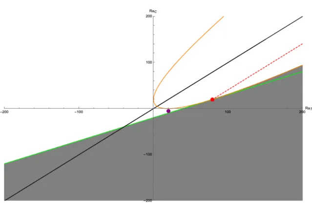
Figure 10: Showing point (175, 70) in purple between the oscillatory and direct instability regions.

(35)

equation (69) forα, derived directly from the imaginary equation,

α= −J 2

n(1 +Le) +a2Le(RaT −RaC) 2JnLe

≈11.45 (87)

and plugging this into the real equation (52) we get β2 _{≈ −}₁₀₈_._{9, which is not an} allowable value for eigenvalues, since β is real by definition. By using our second boundary on oscillatory behavior from equation (85), we see that

2π2−2√2πpRaT +RaT = 2π2−2 √

2π√175 + 175 ≈77.19>75 =RaC (88)

This implies that it is below the allowable oscillatory region, given by the orange curve in Figure (10) but within the directly unstable regime. Therefore, the complete two-dimensional stability analysis needs all restrictions given above to give a true picture of what happens in double diffusion. This complete solution can be extended into the third dimension when you add a third component.

5.5.2 Interpretation of Two-Dimensional Stability Plot

Understanding the physical interpretation of the two dimensional case, we can expand the results to see what occurs when another component is added.

Case (1): In the case where hot, salty fluid is on top of cold, fresh fluid, the experiment lies within the bottom left quadrant. If the solution is stably stratified from a static stand point, then it would lie above the black line in Figure (9). Since the thermal diffusivity is much larger than the solute diffusivity, as a fluid parcel is displaced upwards, it would quickly equilibrate to the surrounding temperature of the stable thermal field, yet still remain fresh, allowing it to continue upwards towards even warmer fluid. This is the direct mode of instability between the green and black lines.

(36)

the orange line, the solution becomes directly unstable. This suggests that there is a small region where the stability of the salt is not strong enough to create oscillations, allowing the thermal field to control the unstable behavior.

Case(3): For most of the statically stable situations, especially those that lie within Quadrant 2, the solution is both thermally and solutably stable. Therefore there are no oscillation or fingering behaviors. This would be the case where cold, salty fluid is under warmer fresh fluid.

5.5.3 Three components

Returning to the three-component case with equation (50), let σ = α+iβ. Then (50) can be split into real and imaginary parts. Where the real equation is

Jnαa2

Led RaCd−RaT

+LeSa RaCSa−RaT

+LeSaLed RaCSa+RaCd

+J_n2

a2 LeSaRaCSa +LedRaCd−RaT

+ LeSa+Led+LeSaLed

(α2−β2)

+JnαLeSaLed(α2−3β2) +Jn4+J 3

n 1 +LeSa+Led

α

+a2LeSaLed RaCSa +RaCd−RaT

(α2−β2) = 0

(89)

and the imaginary

0 =β

J_n3 1+LeSa+Led

+2J_n2 LeSa+Led+LeSaLed

α+2a2LeSaLed RaCSa+RaCd−RaT

α

+Jnα a2

Led RaCd−RaT

+LeSa RaCSa−RaT

+LeSaLed RaCSa+RaCd

+LeSaLed(3α2−β2)

!

(90)

Solving these equations, gives us direct and oscillatory regions in the three-dimensional (RaT, RaCSa, RaCd).

Case 1: β = 0 The factor β gives one zero of the solution. Then the equation for neutral stability becomes

RaT −RaCSaLeSa−RaCdLed=

J2 n

(37)

This solution reduces to the two-dimensional case discussed in the previous section, but understanding the stability of the rest of the system, requires solving for the cubic roots of α. We can find these using the analytical formula for cubic roots created by Tartaglia and Cardano. By finding where these roots are positive and real with respect to the parameter space, we can find the regions of direct instability. In order to simplify this calculation, the horizontal wavenumber was set toπ, as was derived in the two-component case. We will not show that this is the minimum wave number for the three-component case, but will use it as a placeholder for farther analysis. By setting a to π and therefore, Jn to 2π2 in the first node, we can reduce the equations considerably. We also chose values for the Lewis numbers, such that

LeSa = 2 (the same as used in the two-component case) and Led = 3. Then we are only solving,

12π2α3+ 44π4+ 6π2(RaCSa +RaCd −RaT)

α2 + 16π8+ 8π6RaCSa + 12π6RaCd−4π

6_Ra

T + 48π6+ 16π4RaCSa+ 18π 4_Ra

Cd−10π 4_Ra

T

α = 0 (92)

(38)

(39)

Algorithm 1 Algorithm for Direct Instabilities

1: Set β = 0 in Equation (92)).

2: Set parameters values for Jn, a, LeSa, and Led. (Values used for this analysis shown below.)

Jn= 2π2(minimum value)

a=π (minimum value)

LeSa = 2

Led= 3

3: Set precision,ε, for finding roots. (Value used for this analysis shown below.)

ε= 10−20

4: Solve Equation (92) for 3 α roots: Root1[RT, R1, R2], Root2[RT, R1, R2], Root3[RT, R1, R2]

5: for (RT, R1, R2) in Range[ -n, n , h] do

6: if Abs Im(Root[RT, R1, R2])< ε and Re(Root[RT, R1, R2]) > εthen

7: Point is unstable =⇒ Append (RT, R1, R2) to list

8: else

9: Point is stable =⇒ Continue 10: end if

(40)

(a)RaCd =−5. (b)RaCd = 5.

(c) RaCd =−20. (d)RaCd = 20.

(e) RaCd =−50. (f) RaCd = 50.

Figure 12: Perturbed RaCd values using Three-Component Direct Instability Algo-rithm.

(41)

solved for the β2 _{term within. Using the same variables as above,}

β2 = 48π6 + 16π4RaCSa + 18π 4_Ra

Cd−10π 4_Ra

T

+ 88π4+ 12π2(RaCSa +RaCd −RaT)

α+ 36π2α2 >0 (93)

This gives a quadratic in terms of α that must be greater than zero for oscillatory modes of instability. Solving this with the quadratic formula, we get two roots. Let

Ra= (RaCSa+RaCd−RaT),then,

α=−72π4

22π2+ 3Ra±

q

52π4_{+ 9}_Ra2₋₆_π2₍₂_Ra

CSa + 5RaCd−7RaT)

(94)

If you plug in the equation for β2 into the real equation (89), you get a cubic n terms of α. Solving these roots as we did for the direct case, we can again check to see where they are real valued and positive. Because of the second condition, though, oscillations only occur whenβ2¿ 0. Since these are both equations in terms of the parameters, we can loop through within a given range to find the oscilla-tory range.Either the discriminant is positive or if negative other conditions must be applied. In equation (93), the leading term is positive, which indicates that the quadratic is concave up. Therefore, when the discriminant is positive, the two roots given by equation (94) are ordered such that the positive square root is always larger than the negative. Then we can check to see if the cubic root ofαis greater than the larger β root or smaller than the smaller one. This along with ensuring that α and the discriminant are real-valued and positive, gives a set of Rayleigh values where oscillatory behavior occurs.

For example, consider the point (RaT, RaCSa, RaCd) = (130,50,0), which, from the two-component case, we know lies in the blue oscillatory region. By graphing β2

(42)

(a) Oscillatory: (RaT, RaCSa, RaCd) = (130, 50,0).

(b) Not Oscillatory: (RaT, RaCSa, RaCd) = (135, 50,0).

(c) Oscillatory: (RaT, RaCSa, RaCd) = (135, 50,3).

(43)

Figure 14: Three-component script reduced to two-component case for oscillatory instability.

This was done using a Mathematica script following Algorithm 2, as shown in Appendix C. These parameters can then be plotted in three-dimensions. If we reduce to the two dimensional case by setting RaCd = 0, we rediscover the two-component oscillatory instability region. Using Algorithm 2 we can look at perturbed values of

(44)

Algorithm 2 Algorithm for Oscillatory Instabilities

1: Create function for Equation (93) and (89))

2: Set parameters values for Jn, a, LeSa, and Led. (Values used for this analysis shown below.)

Jn = 2π2

a=π LeSa = 2

Led= 3

3: Set precision,ε, for finding roots. (Value used for this analysis shown below.)

ε= 10−20

4: Solve Equation (89) for 3 α roots: Root1[RT, R1, R2], Root2[RT, R1, R2],

Root3[RT, R1, R2]

5: Solve Equation (93) for 2 α roots: βRoot+[RT, R1, R2], βRoot−[RT, R1, R2] 6: Find discriminant of Equation (93): disc[RT, R1, R2]

7: for (RT, R1, R2) in Range[ -n, n, h] do

8: if Abs (Im (Root[RT, R1, R2]) ) < ε and Re(Root[RT, R1, R2])> ε then 9: Point is unstable =⇒ Continue

10: if disc[RT, R1, R2]< ε then

11: Point is Oscillatory =⇒ Append (RT, R1, R2) to list 12: else if disc[RT, R1, R2]< ε then

13: if βRoot+[RT, R1, R2]< Re(Root[RT, R1, R2]) then 14: Point is Oscillatory =⇒Append (RT, R1, R2) to list 15: else if βRoot−[RT, R1, R2]> Re(Root[RT, R1, R2]) then

16: Point is Oscillatory =⇒Append (RT, R1, R2) to list

17: else

18: Point is not Oscillatory =⇒ Continue

19: end if

20: end if 21: else

22: Point is Stable =⇒Continue 23: end if

(45)

6 Discussion

In diffusion experiments set up as these experiments were, with fresh fluid strati-fied over dyed, salty fluid, one would expect the salt and dye to diffuse upwards to the lower concentration gradient in the fresh fluid. This would cause the density and viscosity to increase in the top and decrease in the bottom. The experiments measuring temperature over time, show that the temperature consistently rose by at least a degree in the top and the bottom over time. A temperature increase causes the density to drop much more than the slower, upward diffusion of salt causes it to increase. This is seen in both the extended and the zoomed in NaCl experiments. It is also a factor in the NaI experiments, except that the salt did not diffuse. While most experiments had a stable system of warm fluid over cold fluid, there were a few cases where the opposite held, but there was not enough data to show if this unstable regime changed the outcome of the stability. In any case, one can see that temperature is a strong factor in determining the outcome of the diffusion.

The second component of the diffusion, the dye, can visually be seen diffusing quickly throughout the solution. The dye is what we use to visualize the fingering and os-cillations. While the dye does appear with these instabilities, a study by Camassa, McLaughlin, and Valchar found this fingering effect to happen without dye, and when dye was added to either the top or the bottom layer [11]. This suggests that this component is not crucial to the instability regime. The dye must be impacted by some other diffusing factor affecting the flux within the solution and creating the fingering and oscillatory behavior.

(46)

(a)RaCd =−5. (b)RaCd = 5.

(c) RaCd =−20. (d)RaCd = 20.

(47)

Sodium and Potassium Iodide have densities of 3.67 and 3.12 g/cm3 _{respectively,} compared to the Chloride based salts which range from 1.98 to 2.16 g/cm3. This might indicate it is hard for small parcels of the denser salts to break away from the whole to allow the fingering or oscillatory behavior. Since Iodide based salts are denser, it takes less salt mass added to create the same density stratification. Fewer salt particles diffused within the bottom layer could change the way that the diffusion occurs.

(48)

Figure 16: Periodic Table with Studied Elements in Red [6].

One such alternative could be the impact of Chlorine on dye. Chlorine is often used to strip color from things such as hair or clothing. It is possible that there is some reaction between the dye and the Chlorine that causes the instabilities we see. Bendig, Maier, and Vetter [2] explain that Bromine, directly below Chlorine on the periodic table (see Figure (16)), is used to make brominated vegetable oil, an emulsifying agent in many soft drinks. With a density of 1.33 g/cm3, it mixes with less dense dye or flavor oil to produce an oil with the same density as the environment, in this case the water in soda. As Bromine is the Halogen directly between Chlorine and Iodine, it stand to reason that some of these chemical qualities that allow the Bromine to react with the dye could also be present in Chlorine based salts. On the other hand, it could be Iodine which is similar to Bromine, explaining why the fingering of the dye does not occur with KI, or why the diffusion process takes so much longer than with NaCl and KCl.

(49)

been recorded. While more experimentation would have to be done to show any true range, very rarely were oscillatory and fingering behavior observed in solutions where the top density was less than 1.18 g/cm3_{. Since very little oscillatory and fingering} behavior was observed in the extended NaCl trial, we can also conjecture an upper bound around 1.20g/cm3. Within this range, instabilities were not guaranteed, but most often occurred with varying intensity.

7 Conclusion

The stability analysis shows that while there are regions where oscillations and fin-gering occur, the absence of an adverse gradient implies that there must be another factor involved in the salt-stratified experiments. For future work, it would be best to study the other cases of diffusion outlined in Section 6.5.3 to see if they align more closely with the theoretical results, and explore other salts such as Bromine. There was no clear correlation within the studied density ranges corresponding to greater intensity or frequency of unstable behavior, but the solutions exhibiting oscillations or fingering largely fell between ρT op = 1.18g/cm3 and ρT op = 1.20g/cm3. More experiments could better understand the presence and occurrence of the observed behavior over time. There also needs to be a more in depth study into the stability of the three-dimensional case as well as looking into the math involved in the true fluid regime. Most interestingly, we found results that were slightly different from those presented in previous work, including a larger region for direct instabilities and a smaller region for oscillatory instabilities. The results in this analysis and set of ex-periments show that there may be a larger problem behind the observed instabilities, but without farther research we can only conclude that multi-component diffusive convection cannot be the only root of the problem.

References

[1] Anderson, D. (2016) Double diffusive convection in a porous layer. Notes on Industrial Mathematics (Math 680). George Mason University. 149-156. [2] Bendig, P., Maier, L., Vetter, W. (2012) Brominated vegetable oil in soft drinks

– an underrated source of human organo-bromine intake. Food Chem. 133.3, 678-682.

(50)

[4] Mei, C.C. (2002) Notes on 1.63 Advanced Environmental Fluid Mechanics.

[5] Nield, D. and Bejan, A. (2013) Double Diffusive Convection. Convection in a Porous Media. Springer 4, 425-468.

[6] Periodic Table of Elements. (2019) Science Notes and Projects.

[7] Stern, M. E. (1960) The ‘salt fountain’ and thermohaline convection. Tellus 12, 172-175.

[8] Stommel, H., Arons, A.B. and Blanchard,D. (1956) An oceanographers curios-ity: the perpetual salt fountain. Deep-Sea Res. 3, 152-153.

[9] Straughan, B. (2004) Multi-Component Convection Diffusion. The Energy Method, Stability, and Nonlinear Convection.Springer, 238-268.

[10] Tracey. J. (1996) Multi-component convection-diffusion in a porous medium. Thesis for Department of Mathematics, U of Glasgow.

[11] Camassa, R., McLaughlin, R. ,Valchar, K., Stratified diffusion experiments. Joint Applied Math and Marine Science Fluids Lab.

[12] Veronis G. (1965) On finite amplitude instability in thermohaline convection.

J. Mar. Res. 23, 1-17.

[13] Veronis G. (1968) Effect of a stabilizing gradient of solute on thermal convec-tion. J. Fluid Mech. 34, 315-336.

(51)

Appendices

A

Diffusion Experiments by Camassa et al. [11]

(52)

B

Experimental Measurements and Plots

B.1 KI

(53)

B.2 NaI

(54)

B.3 KCl

(55)

B.4 NaCl

(56)

(57)

(58)

(59)

(60)

ThreeComponents

rel=J4+a2J2L1 R1+a2J2L2 R2-a2J2RT+J3α+J3L1α+J3L2α+a2J L1 R1α+

a2_{J L1 L2 R1}_α₊_a2_{J L2 R2}_α₊_a2_{J L1 L2 R2}_α_-_a2_{J L1 RT}_α_-_a2_{J L2 RT}_α₊_J2_L1_α2₊

J2_L2_α2₊_J2_{L1 L2}_α2₊_a2_{L1 L2 R1}_α2₊_a2_{L1 L2 R2}_α2_-_a2_{L1 L2 RT}_α2₊_{J L1 L2}_α3_-_J2_L1_β2

-J2_L2_β2_-_J2_{L1 L2}_β2_-_a2_{L1 L2 R1}_β2_-_a2_{L1 L2 R2}_β2₊_a2_{L1 L2 RT}_β2_-_{3 J L1 L2}_{α β}2

J4₊_a2_J2_{L1 R1}₊_a2_J2_{L2 R2}_-_a2_J2_RT₊_J3_α₊_J3_L1_α₊_J3_L2_α₊_a2_{J L1 R1}_α₊_a2_{J L1 L2 R1}_α₊

a2_{J L2 R2}_α₊_a2_{J L1 L2 R2}_α_-_a2_{J L1 RT}_α_-_a2_{J L2 RT}_α₊_J2_L1_α2₊_J2_L2_α2₊

J2_{L1 L2}_α2₊_a2_{L1 L2 R1}_α2₊_a2_{L1 L2 R2}_α2_-_a2_{L1 L2 RT}_α2₊_{J L1 L2}_α3_-_J2_L1_β2

-J2_L2_β2_-_J2_{L1 L2}_β2_-_a2_{L1 L2 R1}_β2_-_a2_{L1 L2 R2}_β2₊_a2_{L1 L2 RT}_β2_-_{3 J L1 L2}_{α β}2

img=J3β+J3L1β+J3L2β+a2J L1 R1β+a2J L1 L2 R1β+a2J L2 R2β+

a2_{J L1 L2 R2}_β_-_a2_{J L1 RT}_β_-_a2_{J L2 RT}_β₊_{2 J}2_L1_{α β}₊_{2 J}2_L2_{α β}₊_{2 J}2_{L1 L2}_{α β}₊

2 a2_{L1 L2 R1}_{α β}₊_{2 a}2_{L1 L2 R2}_{α β}_-_{2 a}2_{L1 L2 RT}_{α β}₊_{3 J L1 L2}_α2_β_-_{J L1 L2}_β3_{  β} 1

β J

3_β₊_J3_L1_β₊_J3_L2_β₊_a2_{J L1 R1}_β₊_a2_{J L1 L2 R1}_β₊_a2_{J L2 R2}_β₊

a2_{J L1 L2 R2}_β_-_a2_{J L1 RT}_β_-_a2_{J L2 RT}_β₊_{2 J}2_L1_{α β}₊_{2 J}2_L2_{α β}₊_{2 J}2_{L1 L2}_{α β}₊

2 a2_{L1 L2 R1}_{α β}₊_{2 a}2_{L1 L2 R2}_{α β}_-_{2 a}2_{L1 L2 RT}_{α β}₊_{3 J L1 L2}_α2_β_-_{J L1 L2}_β3_

FindingUnstableValuesforDirectMode

Collect[rel/.{β → 0, R2→ 0},α]

J4₊_{2 a}2_J2_R1_-_a2_J2_RT₊__{6 J}3₊_{8 a}2_{J R1}_-_{5 a}2_{J RT}_{ α}₊__{11 J}2₊_{6 a}2_R1_-_{6 a}2_RT_{ α}2₊_{6 J}_α3

dirR[RT_, R1_, R2_] =Collect[rel/.β → 0/.{J→2*Pi^2, a→Pi, L1→ 2, L2→ 3},α]

16π8+8π6R1+12π6R2-4π6RT+48π6+16π4R1+18π4R2-10π4RT α+

44π4+6π2R1+6π2R2-6π2RT α2+12π2α3

αRootsofdirectmode

dirRoot1[RT_, R1_, R2_] =α/. Solve[dirR[RT, R1, R2]⩵0,α][[1]];

Whentheαrootsarepositiveandreal,thesystemisdirectlyunstable:

n=200;(*checking values in the range of this n3 space*)

h = 1;(*stepping by h*)

r =Range[-n, n, h];

r1vals2D = {};

Do[rt = r[[j]];

r1 = r[[k]];

If[Abs[Im[N[dirRoot1[rt, r1, 0]]]] <10^-16 && Re[N[dirRoot1[rt, r1, 0]]] >10^-16,

(61)

Checking2Dcaseforeachroot

r =Range[-n, n, h];

r1vals2D = {};

Do[rt = r[[j]];

r1 = r[[k]]; If[Abs[Im[N[dirRoot1[rt, r1, 0], 40]]] <10^-20 &

Re[N[dirRoot1[rt, r1, 0], 40]] >10^-20, AppendTo[r1vals2D,{rt, r1}],

Continue],{j, 1, Length[r], 1},{k, 1, Length[r], 1}]

r =Range[-n, n, h];

Do[rt = r[[j]];

r1 = r[[k]]; If[Abs[Im[N[dirRoot2[rt, r1, 0], 40]]] <10^-20 &&

r =Range[-n, n, h];

Do[rt = r[[j]];

r1 = r[[k]]; If[Abs[Im[N[dirRoot3[rt, r1, 0], 40]]] <10^-20 &

2019_Whitley.pdf

Multi-Component Diffusion Study and Stability

Analysis

Victoria Whitley

April 8, 2019

Contents

1

Introduction

2

Background

3

Diffusion Experiments

4

Results

4.1

Potassium Iodide (KI)

4.2

Sodium Iodide (NaI)

4.3

Potassium Chloride (KCl)

4.4

Sodium Chloride (NaCl)

5

Theory

5.1

Initial Conditions and Governing Equations

5.2

Non-dimensional Equations

5.3

Steady Base State

5.4

Disturbance Equations

5.5

Stability Analysis

6

Discussion

7

Conclusion

References

Appendices

A

Diffusion Experiments by Camassa et al. [11]

B

Experimental Measurements and Plots

B.1

KI

B.2

NaI

B.3

KCl

B.4

NaCl