TarekZikry_SeniorHonorsThesis.pdf

(1)

(2)

Abstract

(4)

Acknowledgments

(5)

Introduction

Live cell imaging is a technique for the observation of living cells using time-lapse microscopy. It allows the study of individual and population cellular dynamics and as such, has revealed a staggering complexity and heterogene-ity of cellular processes. For example, cells can be studied for characteristics such as the abundance of proteins affecting stem cell fates [23] or activity of proteins marking quiescence [20]. With recent advancements in microscopy technology, time-lapse data can be gathered at higher volumes than ever before [6]. However, a severe bottleneck has emerged in the difficulty in pro-cessing the increasing amount of cellular data due to a lack of automated live cell image analysis algorithms. Through the application of machine learn-ing tools, the efficiency of image analysis can be improved upon and the throughput of live-cell data can be increased.

Kinases are enzymes responsible for the phosphorylation of other proteins. They play a crucial role in the regulation of cellular signal processing [12]. When a cell is perturbed, functional information such as stimulus intensity and frequency can be encoded in a temporal kinase activation pattern, mak-ing kinases a crucial point of research in modern biology [16]. Within an isogenic cell line, individual cells can have different responses to stimuli, re-sulting in divergent kinase behaviors within neighboring cells, underscoring a need to track kinases at the single-cell level [16].

(6)

types of CDKs serve as markers for stages of the cell cycle. For example, increases in CDK2 indicate that a cell is getting ready to begin a new cycle. Conversely, suppression of CDK2 activity indicate that a cell is entering a quiescent, or G0-like state. When CDK2 is not active, there is no phos-phorylation of marker DNA helicase B fused to yellow fluorescence protein mCherry (DHB-mCherry), and the fluorescence signal remains localized in the nucleus. When CDK2 becomes active, phosphorylation of DHB-mCherry occurs and the signal becomes localized only in the cytoplasm of the cell [20]. Therefore, the cytoplasmic-to-nuclear ratio Cyt/Nucl obtained from DHB-mCherry fluorescence can be used to determine CDK-based transition states in a cell.

In order to accurately quantify Cyt/Nucl ratio, the nuclear region of each cell must be segmented; that is, the boundary of the nuclear must be delineated. The standard way to segment nuclei is using a constantly expressed nuclear reporter. This could be a protein that is omnipresent in the nucleus, such as proliferating cell nuclear antigen (PCNA), or a fluorescent stain called DAPI could be used, which requires cells to be fixed. The nuclear region is then segmented through time-consuming processes that involves waterhsedding and thresholding using software such as CellProfiler [5]. To use signals from these markers requires the addition of a specific fluorescence channel in live cell microscopy. A general maximum of three channels can be added, as with each channel added, more light is exposed to the cells, and they can become damaged and even killed.

However, by tracking CDK2 activity alone, it should be possible to seg-ment cellular nuclei without the use of a nuclear marker. As CDK2 becomes active and localizes in the cytoplasm, it leaves a ‘hole’ in the nucleus observ-able visually through the kinase signal. Through the use of machine learning, it should be possible to teach a computer to segment the nucleus only based on the kinase signals, simultaneously reducing phototoxicity, freeing fluores-cence channels for live-cell imaging, and fully automating the segmentation of cellular nuclei.

(7)

are clustering, regression, and classification. However, every machine learn-ing algorithm needs the same components to function. You must have a data to train your algorithm, a model to represent your data, an objective func-tion to evaluate predicfunc-tion accuracy, and an optimizafunc-tion algorithm to tune your model parameters and reduce the objective function with the ultimate goal of generalizing your model for further usage [7].

A subfield of machine known as “deep learning” focuses on learning stract data representations on multiple levels [2]. “Deep” refers to the ab-stract notion of forming an understanding of an advanced concept through stacking simpler representations atop each other. These stacks are referred to as the hidden layers mapping the input to the output, with each layer rec-ognizing a more complicated feature [19]. Through the backpropagation of model error, deep learning tunes these internal model parameters, or weights, which are then used to find complex patterns within a dataset and relate one layer to the next [13]. Deep learning achieved a significant breakthrough in 2012 Large Scale Visual Recognition Challenge (LSVRC). Researchers Alex Krizhevsky, Ilya Sutskever, and Geoffrey E. Hinton from the University of Toronto used the 15 million image dataset ImageNet to create a new deep con-volutional neural network that would later be called AlexNet. AlexNet took advantage of graphical processing units (GPUs) for training of the model. The added power and capability of the GPUs allowed for the creation and training of deeper models which were able to exploit the breadth of training data. This, in addition to other now-crucial operations such as the novel Rectified Linear Units (ReLU) in their architecture, led the team to reduce classification error 10.8% over the next best competitors [11].

(8)

recog-nition [9] to robotics [17]. CNNs are especially apt at image classification and object recognition tasks. Convolution filters are ideal for recognizing localized spatial features and have the added benefit of reducing trainable parameters from one layer to another, reducing computation time to allow for longer training. Neural networks can recognize common features through the identification of complex linking patterns autonomously. The more labelled pictures the network is given, known as supervised learning, the better the network will become at identifying these features. For instance, in order to teach a deep CNN to recognize a picture of a car in a parking lot, the first layer might recognize the horizon in the background. Next, it might distin-guish the parking lot from the car and then move on to recognizing patterns within the car itself: the hood, wheels, windows, and trunk. Eventually, the understanding of each individual feature, or layer, will form a hierarchy for the basis of machine learning for the network to be able to recognize and isolate a car.

In 2015, the CNN framework U-Net was created for biomedical image segmentation. By upsampling the data into higher resolution outputs, U-Net expands the captured context from the fully-convolutional pooling to enable higher localization accuracy [18]. Due to this uniquely symmetric architecture between the encoding and decoding channels, the U-Net archi-tecture won the ISBI Cell Tracking Challenge 2015, the 2015 EM Segmen-tation Challenge and more recently, the 2018 Data Science Bowl. Further comparisons show that U-Net is faster and more accurate than another CNN DeepCell, while widening the gap between processing methods such as Cell-Profiler [4]. U-Net has already been used in various biomedical image seg-mentation applications such as brain tumor detection [8] and knee cartilage segmentation [14].

(9)

Materials and Methods

4.1 Microscopy

The cell line RPE-DHB was a generous gift from Juanita Limas of the Jean Cook Lab at UNC-Chapel Hill. RPE-hTert cells were obtained from the American Type Culture Collection (ATCC) then authenticated by STR pro-filing and confirmed to be mycoplasma free. Cells were then passaged in Dul-becco’s modified Eagle’s medium (DMEM, Sigma) and supplemented with 10% fetal bovine serum (FBS, Sigma), 1x Pen/Strep, and 4mM L-glutamine and incubated at 37◦C in 5% CO2. First, PCNA-mTurq was transduced in RPE1-hTERT cells virally, then sorted for medium expression, next DHB-mCherry [20] was added and selected with Zeocin.

To prepare for imaging, cells were plated on glass-bottom plates (Cellvis #1.5) before the experiment began. Cells were washed with PBS, fixed with 4% paraformaldehyde (Electron Microscopy Sciences) for 15 minutes at room temperature and stained with DAPI. Imaging was performed using a Nikon Ti Eclipse inverted microscope using Plan Apochromat dry objective lenses 20x (NA 0.75). Images were recorded using an Andor Zyla 4.2 sCMOS detector with 12-bit resolution and converted to 8 bit resolution before the analysis. All filter sets were from Chroma: DAPI - 395/25 nm; 425 nm; 460/50 nm (excitation; beam splitter; emission filter), mCherry - 560/40 nm; 585 nm; 630/75 nm.

4.2 Dataset

(10)

4.3 MB. To create the binary ground truth segmentation masks, the DAPI images were watershedded and opened using the SciKit-Image (Skimage) im-age processing packim-age, version 0.13.1 in Python 3.6. Then using Imim-ageJ, the masks were compared to the DAPI stain and any merged masks were man-ually corrected through separation with a black line. All images were then tiled into four 1024x1024 images to counteract memory issues with the GPU. In total, we had 544 original training pairs consisting of a DHB-mCherry im-age and the corresponding ground truth nuclear segmentation mask. This data was later supplemented through data augmentation. Original training images and masks were morphologically transformed with rotations, mirrors, and light zooms, shears and skews using the Python image augmentation library Augmentor to create 80 randomly chosen 2048x2048 images and sub-sequently 320 tiled images as additional training pairs, resulting in a total training set of 864 images. Each operation was assigned a probability of be-ing used and a range of values. Rotations were assigned an 80% probability with a range of [-5,5]. Horizontal and vertical flips were assigned probabil-ities of 40%. Random zooms were assigned a probability of 50% with area coverage of 95%. Shears had a 20% probability with range of values in [-8,8] for left-right shears. Skews were assigned a 20% probability with a maximum magnitude of 0.15.

4.3 Model and training

(11)

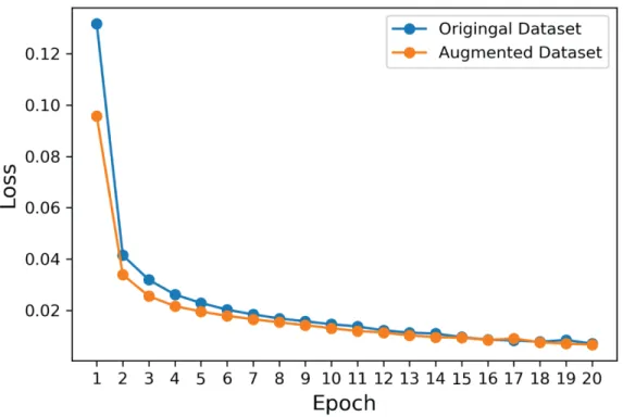
1 hour and 45 minutes over the original dataset and approximately 3 hours over the augmented dataset.

Figure 4.1: Loss function changes during training.

4.4 Evaluation of segmentation

J(A, B) = |A∪B |

|A∩B |

Figure 4.2: Jaccard index between two sets A and B.

(12)

(FN). A true positive is defined as the number of prediction-target mask pairs above the specified Jaccard threshold. A false positive is defined as a predicted mask with no ground truth object and a false negative is a ground truth mask with no predicted mask. Recall and precision (formulas shown in Figure 4.3) parameters were calculated for each Jaccard index threshold value. In the analysis of recall and precision, the objects were stratified based on CDK2 sensor ratio values defined for true positive objects (in ground truth mask for recall analysis and in model output mask for precision analysis).

P recision= T P

T P +F P Recall=

T P T P +F N

Figure 4.3: Precision and recall definitions.

(13)

Results

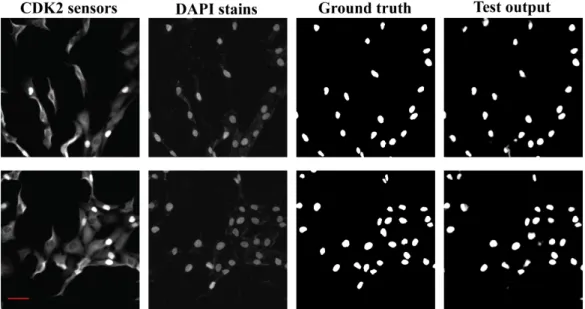
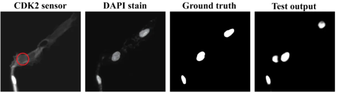
Figure 5.1: Two examples of fluorescent images (DAPI and CDK2 sensor) together with the comparison of ground truth segmentation masks and model output for the same fields of view. Scale bar = 50 µm.

(14)

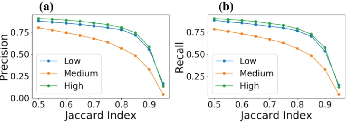
Figure 5.2: Precision and recall rates calculated based on increasing Jaccard index threshold values for cells with low, medium, and high CDK2 activity levels.

(15)

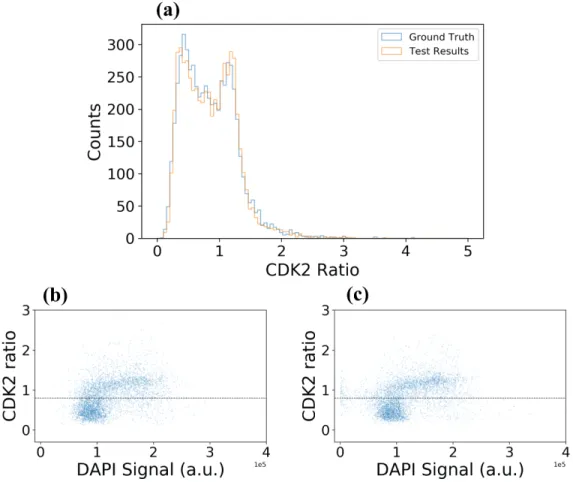
Figure 5.3: a. Comparison of CDK2 ratio distributions based on ground truth and model output masks. b, c. Total DAPI signal vs. CDK2 ratio for ground truth (b) and predicted nuclear regions (c). Vertical lines indicate arbitrary threshold (at the level of 0.8) between cells positioned early or late in the cell cycle.

(16)

(17)

Discussion

We have shown in this thesis that a U-Net type neural network can be trained to successfully segment nuclear regions based on images of a translocating biosensor. Most notably, the achieved quality of segmentation enables us to calculate the correct distribution of CDK2 activity among cells in a het-erogeneous population. This success may be attributed to the fact that the majority of segmentation errors occur in the population of cells with the intermediate CDK2 activity levels. In these cells, the biosensor is equally distributed between the nucleus and the cytoplasm, providing little contrast for the proper segmentation. Yet consequently, the lack of contrast in this population also results in a limited measurement error of the CDK2 activity, even in case of significant segmentation errors.

(18)

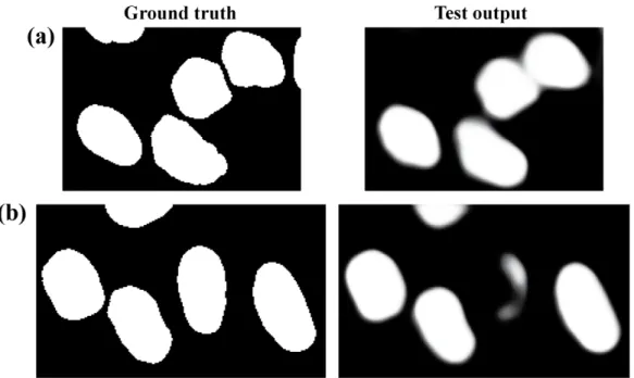
Figure 6.1: Common segmentation errors. a. Example case of merged cells. b. Example case of missed cell in test output.

In order to encourage a network to find the missing thin boundaries, the training could be performed using masks with differentially weighted pix-els. In such prepared masks, boundaries of close objects should be assigned higher weights than the interior pixels of objects, as implemented in the original U-Net report [7]. Moreover, weighted masks could also be utilized to specifically improve the segmentation of the nuclei of cells with interme-diate CDK2 activity and little contrast. Assigning larger weights to pixels belonging to regions with little contrast would effectively force the network to learn how to better segment those regions.

(19)

Figure 6.2: Missed DAPI signal causing erroneous missed cell in ground truth.

In the future, a more thorough vetting of the ground truth segmentation images is necessary to avoid this kind of error compromising the training and confounding the interpretation of the results. Another direction for fu-ture improvement of the segmentation results is fine tuning and estimation of hyperparameters in neural network training, for example annealing of the learning rate during training or testing different loss functions. We were successful in improving the performance of the network by using data aug-mentation and adding transformed images to our training set. This approach could be exploited further and multiple transformations could be added to the training set.

(20)

Conclusion

(21)

Bibliography

[1] Alom, M. Z., Taha, T. M., Yakopcic, C., Westberg, S., Hasan, M., Van Esesn, B. C., Awwal, A. A. S., and Asari, V. K. The history began from alexnet: A comprehensive survey on deep learning approaches. arXiv preprint arXiv:1803.01164 (2018).

[2] Bengio, Y., Courville, A., and Vincent, P.Representation learn-ing: A review and new perspectives. IEEE transactions on pattern anal-ysis and machine intelligence 35, 8 (2013), 1798–1828.

[3] _bvezilic. Nuclei-segmentation. https://github.com/bvezilic/ Nuclei-segmentation, 2018.

[4] Caicedo, J. C., Roth, J., Goodman, A., Becker, T., Karhohs, K. W., Broisin, M., Csaba, M., McQuin, C., Singh, S., Theis, F., et al. Evaluation of deep learning strategies for nucleus segmenta-tion in fluorescence images. BioRxiv (2019), 335216.

[5] _{Carpenter, A. E., Jones, T. R., Lamprecht, M. R., Clarke,} C., Kang, I. H., Friman, O., Guertin, D. A., Chang, J. H., Lindquist, R. A., Moffat, J., et al. Cellprofiler: image analysis software for identifying and quantifying cell phenotypes. Genome biology 7, 10 (2006), R100.

[6] Coutu, D. L., and Schroeder, T. Probing cellular processes by long-term live imaging–historic problems and current solutions. J Cell Sci 126, 17 (2013), 3805–3815.

(22)

[8] Dong, H., Yang, G., Liu, F., Mo, Y., and Guo, Y. Automatic brain tumor detection and segmentation using u-net based fully convo-lutional networks. Inannual conference on medical image understanding and analysis (2017), Springer, pp. 506–517.

[9] Graves, A., and Schmidhuber, J. Offline handwriting recognition with multidimensional recurrent neural networks. InAdvances in neural information processing systems (2009), pp. 545–552.

[10] jvanvugt. pytorch-unet. https://github.com/jvanvugt/ pytorch-unet, 2019.

[11] Krizhevsky, A., Sutskever, I., and Hinton, G. E. Imagenet classification with deep convolutional neural networks. In Advances in neural information processing systems (2012), pp. 1097–1105.

[12] Kudo, T., Jekni´c, S., Macklin, D. N., Akhter, S., Hughey, J. J., Regot, S., and Covert, M. W. Live-cell measurements of kinase activity in single cells using translocation reporters. Nature protocols 13, 1 (2018), 155.

[13] LeCun, Y., Bengio, Y., and Hinton, G. Deep learning. nature 521, 7553 (2015), 436.

[14] Norman, B., Pedoia, V., and Majumdar, S. Use of 2d u-net convolutional neural networks for automated cartilage and meniscus segmentation of knee mr imaging data to determine relaxometry and morphometry. Radiology 288, 1 (2018), 177–185.

[15] Osadchy, M., Cun, Y. L., and Miller, M. L. Synergistic face detection and pose estimation with energy-based models. Journal of Machine Learning Research 8, May (2007), 1197–1215.

[16] _{Purvis, J. E., and Lahav, G.} Encoding and decoding cellular infor-mation through signaling dynamics. Cell 152, 5 (2013), 945–956.

(23)

[18] Ronneberger, O., Fischer, P., and Brox, T. U-net: Convo-lutional networks for biomedical image segmentation. In International Conference on Medical image computing and computer-assisted inter-vention (2015), Springer, pp. 234–241.

[19] Schmidhuber, J. Deep learning in neural networks: An overview. Neural networks 61 (2015), 85–117.

[20] Spencer, S. L., Cappell, S. D., Tsai, F.-C., Overton, K. W., Wang, C. L., and Meyer, T. The proliferation-quiescence decision is controlled by a bifurcation in cdk2 activity at mitotic exit. Cell 155, 2 (2013), 369–383.

[21] Taigman, Y., Yang, M., Ranzato, M., and Wolf, L. Deep-face: Closing the gap to human-level performance in face verification. In Proceedings of the IEEE conference on computer vision and pattern recognition (2014), pp. 1701–1708.

[22] _{Turaga, S. C., Murray, J. F., Jain, V., Roth, F.,} Helm-staedter, M., Briggman, K., Denk, W., and Seung, H. S. Convolutional networks can learn to generate affinity graphs for image segmentation. Neural computation 22, 2 (2010), 511–538.