Available online at www.cuijca.com
International Journal of Computational Analysis
Vol (3), No. (2), pp. 36-47
A FRACTIONAL MODEL FOR DIFFUSION EQUATION USING GENERLIZED FICK’S LAW: EXACT SOLUTION WITH LAPLACE TRANSFORM
Nadeem Ahmad Sheikh1*, Dennis Ling Chuan Ching1, Ilyas Khan2, Afnan Ahmad3 and Syed Ammad3
1Fundamental and Applied Science Department, Universiti Teknologi PETRONAS, Perak 32610, Malaysia 2Department of Mathematics, College of Science Al-Zulfi, Majmaah University, Al-Majmaah 11952, Saudi Arabia. 3Civil and Environmental Engineering Department, Universiti Teknologi PETRONAS, Perak 32610, Malaysia
Keywords:
Caputo fractional derivatives Concentration equation Laplace transformation Fourier sine transformation Exact solutions
ABSTRACT
Fractional calculus is the generalization of classical calculus. Many researchers have used different definitions in their studies. The most common definition is Caputo fractional derivatives operator. In this article the concentration equation is converted to fractional form using the generalized Fick’s law. The fractional partial differential is then transformed with an appropriate transformation. The Laplace and Fourier sine transformations are jointly used to solve the equation. The impact of fractional parameter and Schmidt number is checked on the concentration profile and presented in graphs and tabular form. The results show that diffusion is decreasing with increasing values of Schmidt number.
1 Introduction
Differentiation and integration are often considered discrete operations, in the logic that we differentiate or unify functions once, twice or many times. However, in some cases, it is useful to evaluate derivatives of non-integer order. The idea of fractional calculation is not new. Leibniz raised the possibility of requiring differentiation operations in non-whole orders, in a letter to L'Hospital in 1695[1]. But it was contributed by Liouville, Abel, Heaviside and Riemann, who developed the theory of fractional derivative [2-5]. In many areas, such as chemistry, mechanics and bioengineering, fractional calculations provide a more general and accurate model of the physical system than ordinary calculation [6-9]. Fractional derivatives are also used in electrical circuits, electromagnetic theory and fractal theory for mathematical modeling [10, 11]. Bagley and Torvik [12] gave an early review of taxpayers to the application of fractional calculation to viscoelastic. In the last decade, different techniques have been used to solve fractional differential equations, fractional partial differential equations, fractional whole differential equations and dynamic systems containing fractional derivatives, such as the Adomian decomposition method [13-17], He's variational iteration method [18-20], homotopy perturbation method [21-23], Laplace transform method
[24-26] and other methods [27-29]. Recently, researchers have been trying to reexamine all the classic problems of fluid dynamics, using a fractional calculation approach. However, due to the type of fluid model, especially the Newtonian fluid model, it is not an easy task. In mathematical physics, it is found that special functions are very important for solving solutions of partial differential equations and fractional differential equations, which control the problems of initial value and limit. Many of the special functions of fractional calculations play a very interesting and important role in solving fractional differential equations, such as the Fox’s-H function, the Mittag-Leffler and Wright functions. Wright's functions have been widely used to solve partial differential equations. For the first time it was presented in [30, 31]. Many studies have carried out in the field of fractional calculus, like, Aman et al. [32] studied the fractional model for the graphene based nanofluid and discussed its applications in Solar energy systems. Ali et al. [33] studied the Casson fluid model, using the Caputo fractional derivatives. They have found the closed form solutions and presented the results in terms of special functions. The entropy generation in nanofluids is studied by Saqib et al. [34] using the concept of fractional derivatives. Saqib et al. [35], studied the fractional model for the flow of nanofluid using sodium Alginate as a base fluid. In this paper the effect of different shapes of nanoparticles is discussed in detail. Khan et al. [36] discussed the generalized model for the flow of water based carbon-nanotubes nanofluid. Sheikh et al. [37] presented the comparative study of two fractional derivative operators in their study. The idea of fractional operators is applied to generalize the Casson fluid model in this article. In another paper, Sheikh et al. [38], generalized the model of nanofluid and found the exact solutions. They have discussed the applications in solar collectors. Atangana and Baldik [39], analyzed the ground water flow using the concept of fractional derivatives. Abro et al. [40], studied the MHD flow of nanofluid past a porous medium. They have used the two fractional derivatives approaches to fractionalize the nanofluid models. Saqib et al. [41] discussed the fractional model for the flow of blood with magnetic dusty particles. They have generalized the Brinkman-type fluid model for this analysis.
Mass transfer phenomenon can also be seen in enormous fields of industry, particularly in separation techniques, mass transfer that converts the mixture of substances into the mixtures of distinctive products, which make up the vast majority of industrial production processes, are determined by the physics of mass transfer and their design and operation rest with confidence to a worth considering degree on the knowledge in this field [42, 43]. Heat and mass transfer together are useful in distinctive processes and mechanisms. In engineering, for example, heat and mass transfer is seen in various physical phenomenon including convective and diffusive transport of chemical species within the system.
Keeping in mind the above literature, the idea of fractional derivative with new transformation and using the generalized Fick’s is applied to the concentration equation. The fractional equation with Caputo derivative is then solved by joint application of the Laplace and Fourier sine transformations.
2 Mathematical Formulation
The flow of fluid with mass transfer in a vertical channel is considered. The flow is taken along the x -direction. The y -axis is taken normal to the plate. Initially, the fluid and plates are at rest with uniform concentration C1 respectively. At
0
t , the plate starts motion in its own plane. Atyd, the plate concentration levels raised to C1
C2C g t1
with time t.
The concentration is the functions of (y t, ) only, the equation for mass transfer is given by following partial differential equations [44, 45]:
( , ) ( , ) ,
C y t j y t
t y
(1)
( , )
( , ) C y t ,
j y t D
y
(2)
with the initial and boundary conditions:
1 1
1 2 1
( , 0) , (0, ) ,
( , ) ,
C y C
C t C
C d t C C C g t
(3)
where C is the Concentration, andD is the mass diffusivity.
Introducing the following dimensionless variables:
2 1
2
2 1 2 1
, , C C , , ( ) .
y jd d
t g g t
d d C C D C C
In to Eqs. (1)-(3), we get:
( , ) 1 ( , )
,
Sc
(4)
( , )
( , ) ,
(5)
( , 0) 0,
(0, ) 0, ,
(1, ) g( ),
(6)
where Sc D is the Schmidt number.
2.1.Fractional Model
To develop a fractional model for the mentioned flow problem, the generalized Fick’s is used as under:
1 ( , )
( , ) C ; 0 1,
(7)
01
( , ) ( , )( )
1
( ) * ( , ); 0 1, t
C
tr y t r y s t s ds
t r y t
(8) Here
( ) 1 t t is the singular Power law kernel. Furthermore,
1 1 0 1 1 1 1 1( ) , * 1, ( ) 1,
( ) 1 ( ),
L t t t L
s s
t L t
(9)
here L
. is the Laplace transform, (.)is the Dirac’s delta function and sis the Laplace transform parameter. Using the above properties and the second form Eq. 8, it is convenient to show that0
( , ) ( , ) ( , 0),
C
tr y t r y t r y
(10)
1 ( , )
( , ) C
t
r y t r y t
t
. (11)
Utilizing the definition of Caputo time fractional operator form Eq. (8), we arrived at:
2 1
2
( , ) 1 ( , )
, C t Sc
(12)
To obtain the more suitable form of the last two equation we recall the time fractional integral operator
11
0
1
( , ) * ( ) ( , )( ) ,
t
t r y t r t r y s t s ds
(13)This is the inverse operator of the derivative operatorCt
. . Using the properties from Eq. (9) we have
1
1
, , * *
* * 1* ( ) ( , ) ( , 0),
C C
t r y t t r y t r t
r t r t r y t r y
(14)
t C
r y t
, r y t( , ) if r y
, 0
0. (15)Using the property, 1t r y t
, *r ( )t C tr y t
, ,
Eqs. (12) can be written as:
2 2
1 ( , )
( , ) , C Sc
3 Solution of the Problem 3.1.Concentration Field Using the following transformation
,
,
g
, (17)
Eq. (16) takes the form
2 2
1 ( , )
( , ) ( ) ,
C C
g
Sc
(18)
With the corresponding initial and boundary conditions as ( , 0) 0, (0, ) 0, (1, ) 0.
(19)
Applying the Laplace and Fourier sine transform, we get
12
1
( , ) ( ) ,
n F
s n s sg s
n n
s
Sc
(20)
Inverting the integral transformations of Eq. (20), we have
2, 1
1 0
1 sin
( , ) 2 ,
n
n
n n
g t E t dt
n Sc
(21)The final solution for the concentration equation is
,
,
g
, (22)
4 Results and Discussion
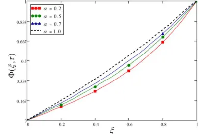
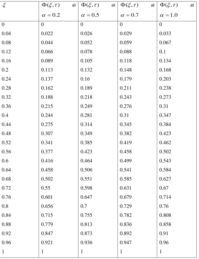
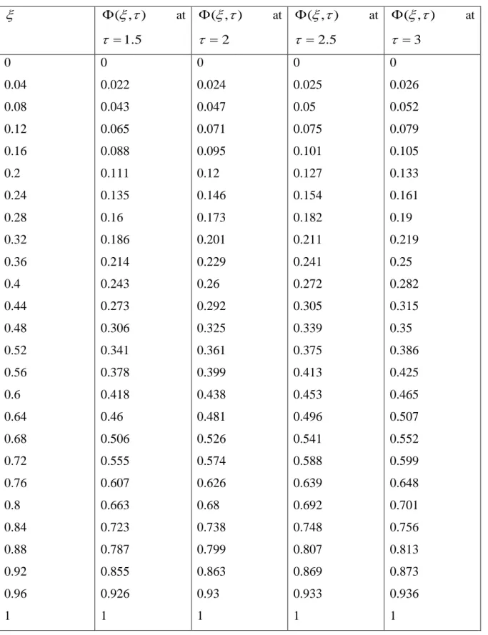
The Caputo time fractional derivative approach is used to generalize the concentration equation and then solved for exact solution using the integral transformed. The impact of different parameters is shown in figures and tables. The impact of fractional parameter is shown in Fig. 1 and Table 1. It is noticed that the concentration of mass particle is increasing with the increasing values of fractional parameter. And is higher for the classical case. Both the figure and table show that the imposed boundary conditions are verified. In order to show the effect of Schmidt number, Fig. 2 and Table 2 are presented, the concentration of mass is decreasing function of Schmidt number. This is because Schmidt number is the ratio of viscosity to mass diffusivity. The variations in concentration profile due to time parameter is shown in Fig. 3 and Table 3. It is noticed that concentration of mass is increasing with increasing time.
5 Conclusion
The Caputo time fractional derivative approach is used to generalize the concentration equation and then solved for exact solution using the integral transformed. The impact of different parameters is shown in figures and tables. The following are the main points extracted from the present study:
1. Concentration is the increasing function of fractional parameter.
2. The higher values of Schmidt number decrease the concentration of mass. 3. The new transformation is more reliable for the exact solutions.
4.
Fig 1: Variations in Concentration profile against for different values of .
Fig 2: Variations in Concentration profile against for different values of Sc.
Table 1: Variations in concentration profile against g( ) 1 for different values of .
( , ) at0.2 ( , ) at 0.5 ( , ) at 0.7 ( , ) at 1.0 0 0.04 0.08 0.12 0.16 0.2 0.24 0.28 0.32 0.36 0.4 0.44 0.48 0.52 0.56 0.6 0.64 0.68 0.72 0.76 0.8 0.84 0.88 0.92 0.96 1 0 0.022 0.044 0.066 0.089 0.113 0.137 0.162 0.188 0.215 0.244 0.275 0.307 0.341 0.377 0.416 0.458 0.502 0.55 0.601 0.656 0.715 0.779 0.847 0.921 1 0 0.026 0.052 0.078 0.105 0.132 0.16 0.189 0.218 0.249 0.281 0.314 0.349 0.385 0.423 0.464 0.506 0.551 0.598 0.647 0.7 0.755 0.813 0.873 0.936 1 0 0.029 0.059 0.088 0.118 0.148 0.179 0.211 0.243 0.276 0.31 0.345 0.382 0.419 0.458 0.499 0.541 0.585 0.631 0.679 0.729 0.782 0.836 0.892 0.947 1 0 0.033 0.067 0.1 0.134 0.168 0.203 0.238 0.273 0.31 0.347 0.384 0.423 0.462 0.502 0.543 0.584 0.627 0.67 0.714 0.76 0.808 0.858 0.91 0.96 1
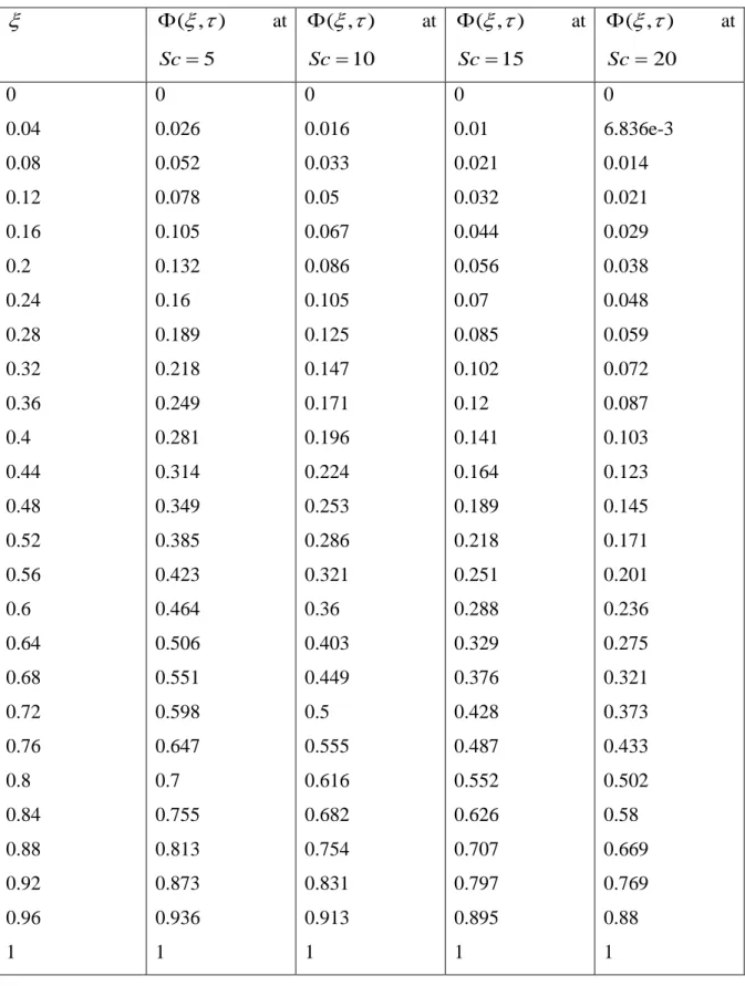
Table 2: Variations in concentration profile against g( ) 1 for different values of Sc.
( , ) at5 Sc ( , ) at 10 Sc ( , ) at 15 Sc ( , ) at 20 Sc 0 0.04 0.08 0.12 0.16 0.2 0.24 0.28 0.32 0.36 0.4 0.44 0.48 0.52 0.56 0.6 0.64 0.68 0.72 0.76 0.8 0.84 0.88 0.92 0.96 1 0 0.026 0.052 0.078 0.105 0.132 0.16 0.189 0.218 0.249 0.281 0.314 0.349 0.385 0.423 0.464 0.506 0.551 0.598 0.647 0.7 0.755 0.813 0.873 0.936 1 0 0.016 0.033 0.05 0.067 0.086 0.105 0.125 0.147 0.171 0.196 0.224 0.253 0.286 0.321 0.36 0.403 0.449 0.5 0.555 0.616 0.682 0.754 0.831 0.913 1 0 0.01 0.021 0.032 0.044 0.056 0.07 0.085 0.102 0.12 0.141 0.164 0.189 0.218 0.251 0.288 0.329 0.376 0.428 0.487 0.552 0.626 0.707 0.797 0.895 1 0 6.836e-3 0.014 0.021 0.029 0.038 0.048 0.059 0.072 0.087 0.103 0.123 0.145 0.171 0.201 0.236 0.275 0.321 0.373 0.433 0.502 0.58 0.669 0.769 0.88 1
Table 3: Variations in concentration profile against g( ) 1 for different values of .
( , ) at
1.5 ( , ) at 2 ( , ) at 2.5 ( , ) at 3 0 0.04 0.08 0.12 0.16 0.2 0.24 0.28 0.32 0.36 0.4 0.44 0.48 0.52 0.56 0.6 0.64 0.68 0.72 0.76 0.8 0.84 0.88 0.92 0.96 1 0 0.022 0.043 0.065 0.088 0.111 0.135 0.16 0.186 0.214 0.243 0.273 0.306 0.341 0.378 0.418 0.46 0.506 0.555 0.607 0.663 0.723 0.787 0.855 0.926 1 0 0.024 0.047 0.071 0.095 0.12 0.146 0.173 0.201 0.229 0.26 0.292 0.325 0.361 0.399 0.438 0.481 0.526 0.574 0.626 0.68 0.738 0.799 0.863 0.93 1 0 0.025 0.05 0.075 0.101 0.127 0.154 0.182 0.211 0.241 0.272 0.305 0.339 0.375 0.413 0.453 0.496 0.541 0.588 0.639 0.692 0.748 0.807 0.869 0.933 1 0 0.026 0.052 0.079 0.105 0.133 0.161 0.19 0.219 0.25 0.282 0.315 0.35 0.386 0.425 0.465 0.507 0.552 0.599 0.648 0.701 0.756 0.813 0.873 0.936 1
REFERENCES
[1]. G. W. Leibnitz, "Letter from hanover, germany, september 30, 1695 to ga l’hospital. Leibnizen Mathematische Schriften," ed: Olms Verlag, Hildesheim, Germany, 1962.
[2]. M. Axtell and M. E. Bise, "Fractional calculus application in control systems," in IEEE Conference on Aerospace and Electronics, 1990, pp. 563-566: IEEE.
[3]. K. Oldham and J. Spanier, The fractional calculus theory and applications of differentiation and integration to arbitrary order. Elsevier, 1974.
[4]. S. G. Samko, A. A. Kilbas, and O. I. Marichev, Fractional integrals and derivatives. Gordon and Breach Science Publishers, Yverdon Yverdon-les-Bains, Switzerland, 1993.
[5]. S. Das, Functional fractional calculus. Springer Science & Business Media, 2011. [6]. R. L. Magin, Fractional calculus in bioengineering. Begell House Redding, 2006.
[7]. Y. A. Rossikhin and M. V. Shitikova, "Applications of fractional calculus to dynamic problems of linear and nonlinear hereditary mechanics of solids," Applied Mechanics Reviews, vol. 50, no. 1, pp. 15-67, 1997.
[8]. A. Carpinteri and F. Mainardi, Fractals and fractional calculus in continuum mechanics. Springer, 2014.
[9]. J. T. Machado, V. Kiryakova, F. J. C. i. n. s. Mainardi, and n. simulation, "Recent history of fractional calculus," vol. 16, no. 3, pp. 1140-1153, 2011.
[10]. B. Mandelbrot, "The fractal geometry of nature," Earth Surface Processes and Landforms, vol. 44, no. 12, pp. 406-406, 1982.
[11]. I. Petráš, Fractional-order nonlinear systems: modeling, analysis and simulation. Springer Science & Business Media, 2011.
[12]. R. L. Bagley and P. Torvik, "A theoretical basis for the application of fractional calculus to viscoelasticity," Journal of Rheology, vol. 27, no. 3, pp. 201-210, 1983.
[13]. S. Momani and N. Shawagfeh, "Decomposition method for solving fractional Riccati differential equations," Applied Mathematics Computation, vol. 182, no. 2, pp. 1083-1092, 2006.
[14]. S. Momani and M. A. Noor, "Numerical methods for fourth-order fractional integro-differential equations," Applied Mathematics Computation, vol. 182, no. 1, pp. 754-760, 2006.
[15]. V. Daftardar-Gejji and H. Jafari, "Solving a multi-order fractional differential equation using Adomian decomposition," Applied Mathematics Computation, vol. 189, no. 1, pp. 541-548, 2007.
[16]. S. S. Ray, K. Chaudhuri, and R. Bera, "Analytical approximate solution of nonlinear dynamic system containing fractional derivative by modified decomposition method," Applied mathematics computation, vol. 182, no. 1, pp. 544-552, 2006.
[17]. Q. Wang, "Numerical solutions for fractional KdV–Burgers equation by Adomian decomposition method," Applied Mathematics Computation, vol. 182, no. 2, pp. 1048-1055, 2006.
[18]. M. Inc, "The approximate and exact solutions of the space-and time-fractional Burgers equations with initial conditions by variational iteration method," Journal of Mathematical Analysis Applications, vol. 345, no. 1, pp. 476-484, 2008.
[19]. S. Momani and Z. Odibat, "Analytical approach to linear fractional partial differential equations arising in fluid mechanics," Physics Letters A, vol. 355, no. 4-5, pp. 271-279, 2006.
[20]. Ζ. Odibat and S. Momani, "Application of variational iteration method to nonlinear differential equations of fractional order," International Journal of Nonlinear Sciences Numerical Simulation, vol. 7, no. 1, pp. 27-34, 2006.
[21]. S. Momani and Z. Odibat, "Homotopy perturbation method for nonlinear partial differential equations of fractional order," Physics Letters A, vol. 365, no. 5-6, pp. 345-350, 2007.
[22]. N. Sweilam, M. Khader, and R. Al-Bar, "Numerical studies for a multi-order fractional differential equation," Physics Letters A, vol. 371, no. 1-2, pp. 26-33, 2007.
[23]. Z. Odibat and S. Momani, "Modified homotopy perturbation method: application to quadratic Riccati differential equation of fractional order," Chaos Solitons and Fractals, vol. 36, no. 1, pp. 167-174, 2008.
[24]. H. Qi and H. Jin, "Unsteady rotating flows of a viscoelastic fluid with the fractional Maxwell model between coaxial cylinders," Acta Mechanica Sinica, vol. 22, no. 4, pp. 301-305, 2006. [25]. T. Wenchang, P. Wenxiao, and X. Mingyu, "A note on unsteady flows of a viscoelastic fluid
with the fractional Maxwell model between two parallel plates," International Journal of Non-Linear Mechanics, vol. 38, no. 5, pp. 645-650, 2003.
[26]. N. A. Shah, D. Vieru, and C. Fetecau, "Effects of the fractional order and magnetic field on the blood flow in cylindrical domains," Journal of Magnetism Magnetic Materials, vol. 409, pp. 10-19, 2016.
[27]. F. Liu, V. Anh, and I. Turner, "Numerical solution of the space fractional Fokker–Planck equation," Journal of Computational Applied Mathematics, vol. 166, no. 1, pp. 209-219, 2004. [28]. S. B. Yuste, "Weighted average finite difference methods for fractional diffusion equations,"
Journal of Computational Physics, vol. 216, no. 1, pp. 264-274, 2006.
[29]. S.-Y. Lee, H. Ke, and Y. Kuo, "Analysis of non-uniform beam vibration," Journal of Sound Vibration, vol. 142, no. 1, pp. 15-29, 1990.
[30]. E. M. Wright, "On the coefficients of power series having exponential singularities," Journal of the London Mathematical Society, vol. 1, no. 1, pp. 71-79, 1933.
[31]. E. Wright, "The generalized Bessel function of order greater than one," The Quarterly Journal of Mathematics, vol. 11, no. 1, pp. 36-48, 1940.
[32]. S. Aman, I. Khan, Z. Ismail, M. Z. Salleh, and I. Tlili, "A new Caputo time fractional model for heat transfer enhancement of water based graphene nanofluid: An application to solar energy,"
Results in Physics, vol. 9, pp. 1352-1362, 2018.
[33]. F. Ali, N. A. Sheikh, I. Khan, and M. Saqib, "Solutions with Wright function for time fractional free convection flow of Casson fluid," Arabian Journal for Science Engineering, vol. 42, no. 6, pp. 2565-2572, 2017.
[34]. M. Saqib, F. Ali, I. Khan, N. A. Sheikh, and A. Khan, "Entropy Generation in Different Types of Fractionalized Nanofluids," Arabian Journal for Science and Engineering, vol. 44, no. 1, pp. 531-540, 2018.
[35]. M. Saqib, I. Khan, and S. Shafie, "Shape Effect in Magnetohydrodynamic Free Convection Flow of Sodium Alginate-Ferrimagnetic Nanofluid," Journal of Thermal Science and Engineering Applications, vol. 11, no. 4, 2019.
[36]. I. Khan, M. Saqib, and A. M. Alqahtani, "Channel flow of fractionalized H2O-based CNTs nanofluids with Newtonian heating," Discrete & Continuous Dynamical Systems - S, vol. 0, no. 0, pp. 769-779, 2018.
[37]. N. A. Sheikh et al., "Comparison and analysis of the Atangana–Baleanu and Caputo–Fabrizio fractional derivatives for generalized Casson fluid model with heat generation and chemical reaction," Results in physics, vol. 7, pp. 789-800, 2017.
[38]. N. A. Sheikh, F. Ali, I. Khan, M. Gohar, and M. Saqib, "On the applications of nanofluids to enhance the performance of solar collectors: A comparative analysis of Atangana-Baleanu and Caputo-Fabrizio fractional models," The European Physical Journal Plus, vol. 132, no. 12, 2017. [39]. A. Atangana and N. Bildik, "The use of fractional order derivative to predict the groundwater
flow," Mathematical Problems in Engineering, vol. 2013, 2013.
[40]. K. A. Abro, A. D. Chandio, I. A. Abro, and I. Khan, "Dual thermal analysis of magnetohydrodynamic flow of nanofluids via modern approaches of Caputo–Fabrizio and Atangana–Baleanu fractional derivatives embedded in porous medium," Journal of Thermal Analysis and Calorimetry, vol. 135, no. 4, pp. 2197-2207, 2018.
[41]. M. Saqib, I. Khan, and S. Shafie, "Generalized magnetic blood flow in a cylindrical tube with magnetite dusty particles," Journal of Magnetism and Magnetic Materials, vol. 484, pp. 490-496, 2019.
[42]. Z. Shao, N. A. Shah, I. Tlili, U. Afzal, and M. S. Khan, "Hydromagnetic free convection flow of viscous fluid between vertical parallel plates with damped thermal and mass fluxes," Alexandria Engineering Journal, 2019.
[43]. A. Hussanan, Z. Ismail, I. Khan, A. G. Hussein, and S. Shafie, "Unsteady boundary layer MHD free convection flow in a porous medium with constant mass diffusion and Newtonian heating,"
The European Physical Journal Plus, vol. 129, no. 3, p. 46, 2014.
[44]. A. Khan, D. Khan, I. Khan, F. Ali, F. U. Karim, and M. Imran, "MHD Flow of Sodium Alginate-Based Casson Type Nanofluid Passing Through A Porous Medium With Newtonian Heating,"
Sci Rep, vol. 8, no. 1, p. 8645, Jun 5 2018.
[45]. A. Khalid, I. Khan, A. Khan, and S. Shafie, "Unsteady MHD free convection flow of Casson fluid past over an oscillating vertical plate embedded in a porous medium," Engineering Science and Technology, an International Journal, vol. 18, no. 3, pp. 309-317, 2015.