Optimum Selection of Modes Set for Adaptive
Modulation and Coding based on Imperfect
Channel State Information
Mehrdad TakiDepartment of Electrical Engineering University of Qom
Qom, Iran E-mail: [email protected]
Reza Mahin Zaeem
- Tehran, Iran
E-mail: [email protected]
Received: September 28, 2016- Accepted: December 19, 2016
Abstract—Complexity issues and limited feedback rate strictly constrain the number of transmission modes in discrete
link adaptation. A new algorithm is designed for selecting an optimum set of modes out of all the possible transmission modes based on the link’s characteristics and the constraints, meanwhile, imperfect channel state information (CSI) is available. The design goal is to maximize the average spectral efficiency and the selection is done using a combination of nonlinear quantization and integer programming. As numerical evaluations for adaptive LDPC or convolutional coded, QAM modulated transmission show, performance of the proposed scheme is considerably improved in comparison with the benchmark schemes.
Keywords-component; Link Adaptation; Adaptive Modulation and Coding; Integer programming
I. INTRODUCTION
Link adaptation is an efficient tool to conquest multipath fading in wireless communication systems where transmission rate is adapted based on the received SNR [1]. In practice, a limited set of modes may be utilized where each mode is implemented with a modulation and a coding scheme resulting in a specific transmission rate, i.e., adaptive modulation and coding (AMC). Obviously, the more the number of transmission modes are, the better the performance of the system would be. However, the implementation of each mode requires the use of appropriate hardware/software in the transmitter and the receiver while the hardware complexity and processing capability are limited especially in user end systems. In addition, another obstacle in which practical systems may be confront is that adapting rate based on perfect
channel state information (CSI) is impossible. That CSI is not existing because of error in channel estimation and time variant essence of channels.
Eventually, the index of appropriate mode must be sent back to the transmitter, as regards, increasing the number of modes would increase the feedback rate, so limited number of transmission modes must be considered.
AMC is implemented in IEEE 802.11 [2] and DVB [3] standards. Not only it is shown that the performance of different systems is improved by using AMC with perfect CSI [4]-[13], but also it can be observed that AMC increase system's performance with imperfect CSI [14]-[15]. In the mentioned articles, a limited number of transmission modes are selected randomly and the selected set remains unchanged, although, by the change of the link’s characteristics or constraints. Based on the author's knowledge, no
method has been presented yet for optimum selection of modes set for AMC transmission.
In this article a new method is presented in which a set with 𝑀 members is optimally selected from all the available transmission modes (a set with 𝑁 modes) to maximize the average spectral efficiency (ASE) of the link. The selection is done based on the PDF of channel’s SNR and the BER constraint. Design is done using a combination of nonlinear quantization and integer programming. At the beginning of the communication, modes set is selected and contracted between the receiver and the transmitter. After that, only the appropriate mode's index will send back to the transmitter. In this case, the required feedback rate is ⌈log2𝑀⌉. In comparison with random selection of the modes or the case where the modes set is unchanged by the link’s characteristics, numerical evaluations indicate that the performance is considerably improved. In the following, in section II, the scheme for optimum selection of modes set is presented. In section III, performance of the proposed scheme is examined using numerical evaluations. Benchmarks are set up as comparison basis to show the efficiency of the proposed algorithm. Finally the paper will be concluded in section IV.
II. OPTIMIZED SELECTION OF MODES SET The goal is to design a scheme for selecting a subset with 𝑀 members (ℳ̃ = {𝑅̃1< 𝑅̃2< ⋯ < 𝑅̃𝑀}) out of all available transmission modes with 𝑁 members (𝒩 = {𝑅̂1< 𝑅̂2< ⋯ < 𝑅̂𝑁}) to maximize ASE of the link. The instantaneous BER, 𝑝𝑒(𝛾̌, 𝑘), is constrained to 𝐵0. If 𝑘 and 𝛾̌, respectively, show the instantaneous rate and perfect SNR of the link, the problem can be formulated as follows,
ℳ̃ = {𝑅̃1, 𝑅̃2, … , 𝑅̃𝑀} =
arg max
ℳ={𝑅1,𝑅2,…,𝑅𝑀}⊂𝒩
𝐴𝑆𝐸 = 𝐸{𝑘}, 𝑘 ∈ ℳ Subject to: {C(1): ‖ℳ‖ = 𝑀
C(2): 𝑝𝑒(𝛾̌, 𝑘) ≤ 𝐵0
1
where ‖ℳ‖ represents the number of the members in the set ℳ. The above problem is a constrained discrete optimization problem that its solution is not straightforward. In the following, after description of channel model and imperfect CSI, at first 1, is reformulated based on the BER constraint. Next, an equivalent continuous problem is solved to obtain insight and compute the upper bound of performance. Finally, the solution of the reformulated problem will be presented.
A. Channel Model and Imperfect CSI
The communication system consists of a single input single output model over a Nakagami flat fading channel. As we supposed to available CSI is not perfect, so the estimated imperfect instantaneous SNR in the receiver would be 𝛾. These two SNRs have a conditional distribution function with a correlation coefficient. Assuming a Nakagami flat fading channel of order 𝜇, the conditional distribution can be stated as follows [13],
𝑓𝛾̌|𝛾= (𝛾̌
𝜌𝛾)
𝜇−1
2 1
𝛤exp (− 𝜌(𝛾+𝛾̌) 𝛤(1−𝜌)) 𝐼𝜇−1(
2
𝛤(1−𝜌)√𝜌𝛾𝛾̌ )
2
where 𝜇 is Nakagami order, 𝛤 represents the average of SNRs (𝛤 = 𝐸{𝛾} = 𝐸{𝛾̌}), 𝜌 = 𝐽02(2𝜋𝑓𝑑𝑇𝑑) is correlation between 𝛾 and 𝛾̌, 𝐽0(. ) is Bessel function of the first type and zero order, 𝑓𝑑 is the Doppler frequency and 𝑇𝑑 is the round trip time of the channel and 𝐼𝜇−1(. ) shows the modified Bessel function of the first type and order of 𝜇 − 1.
B. Problem Reformulation based on the BER constraint for imperfect CSI
In general, to guarantee the BER constraint with perfect CSI, i.e., 𝑝𝑒(𝛾̌, 𝑘) ≤ 𝐵0, it is required that 𝛾̌ ≥
𝑔𝐵0(𝑘) where 𝑔𝐵0(. ) is a function of utilized coding
and modulation scheme [14]. As it is discussed in [14] with imperfect CSI, we just may limit the probability of violation of BER from the required constraint, as follows,
𝑃𝑟𝑜𝑏{(𝑝𝑒(𝛾̌, 𝑘) > 𝐵0)|𝛾} ≤ 𝐵𝑣 3 However, just (1 − 𝐵𝑣) part of this transmission rate is reliable and is considered in the performance evaluation. To this end, it is required that,
𝑔𝐵0(𝑘) ≤ (𝑄1√𝛾 − 𝑄2)2 4
where 𝑄1= 𝜌, 𝑄2= √−(1 − 𝜌) ln(2𝐵𝑣) [14]. The
𝛾𝑚 in 𝑔𝐵0(𝑅𝑚) ≤ (𝑄1√𝛾𝑚− 𝑄2) 2
is the minimum required SNR to satisfy the BER constraint when rate is 𝑅𝑚, 1 ≤ 𝑚 ≤ 𝑀.
With modes set ℳ = {𝑅1< 𝑅2< ⋯ < 𝑅𝑀}, and their corresponding thresholds as 𝛾1< 𝛾2< ⋯ < 𝛾𝑀, ASE is computed as follows,
𝐴𝑆𝐸 = ∑ 𝑔𝐵0−1((𝑄 1√𝛾𝑚− 𝑀
𝑚=1
𝑄2) 2
) ∫ 𝑓𝛾(𝛾)𝑑𝛾 𝛾𝑚+1
𝛾𝑚
5
where 𝑓𝛾(. ) is the probability density function (PDF) of imperfect SNR and 𝑔𝐵0
−1(. )
is the inverse function of 𝑔𝐵0(. ).
There are 𝑁 thresholds corresponding to 𝑁 possible transmission rates as follows,
𝛤̂ = {𝛾̂1< ⋯ < 𝛾̂𝑁}, (𝑄1√𝛾̂𝑛− 𝑄2) 2
= 𝑔𝐵0(𝑅̂𝑛), 1 ≤ 𝑛 ≤ 𝑁; 𝑅̂𝑛∈ 𝒩
6
Thus, 1 may be reformulated as, 𝛤̃ = arg max
Γ={𝛾1<𝛾2<⋯<𝛾𝑀}⊂ Γ̂
𝐴𝑆𝐸(𝛾1, … , 𝛾𝑀) 7 where C(1) in 1 is now considered in the number of selected thresholds and C(2) is provisioned in the relation between the thresholds and the rates as in 4. Problem 7, is an unconstrained discrete optimization that may be solved by checking all the possible answers and select the best one. The number of possible subsets of 𝛤̂ with 𝑀 members is 𝑁!
𝑀!(𝑁−𝑀)!; clearly, complexity of exhaustive search becomes too high when 𝑁 is large.
In the next section, the equivalent continuous optimization problem is solved to obtain analytical insights and in the section after next, solution of 7 is presented.
C. Performance analysis considering continuous form of the optimization problem
In this section, to obtain analytical insight we assume that the modes set in Problem 7 could contains any 𝑀 real values and its members are not obliged to be selected from 𝛤̂ in 6. To solve the equivalent optimization problem. At first step, we need a closed form function for 𝑔𝐵0(. ), then we present the solution.
1) A closed form function to estimate 𝑔𝐵0
The function 𝑔𝐵0(. ) may be computed by analytical performance analysis of the utilized coding and modulation schemes [16]. As the presented analytical bounds are not precise enough, we numerically evaluate the 𝑔𝐵0(𝑅̂𝑛) values by
simulation of the link’s performance. Then, with the help of curve fitting, a continuous function is fit for computing 𝑔𝐵0
−1(𝛾̌)
in a form of 𝐴 ln(𝐵𝛾̌ + 𝐶), where 𝐴, 𝐵 and 𝐶 are constants depending on 𝐵0. The function 𝑔𝐵−10(𝛾̌) shows the maximum transmissible rate which satisfies the BER constraint. We compute 𝑔𝐵0
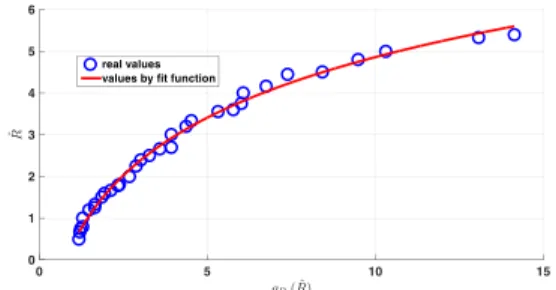
−1(𝛾̌) for different set of rates ( 𝒩 ) with convolutional or LDPC coded QAM modulated modes. In Figures 1 and 2, the values of 𝑅̂𝑛 versus 𝛾̂𝑛 and 𝑔𝐵−10(𝛾̌) are plotted for two selected sets. Evidently, the approximate functions are precise enough. Note that in this stage estimation of 𝑔𝐵0(. ) is based on perfect CSI.
2) Solution of the continuous form of the optimization problem
If rates weren't discrete and instantaneous transmission rate was continuously adapted versus SNR, ASE of continuous rate adaptation based on 5 and 4 would be,
𝐴𝑆𝐸𝑐𝑜𝑛𝑡_𝑟𝑎𝑡𝑒_𝑎𝑑𝑝= (1 −
𝐵𝑣) ∫ 𝐴 ln(𝐵(𝑄1√𝛾 − 𝑄2)2+ ∞
max (1−𝐶𝐵 ,0)
𝐶) 𝑓𝛾(𝛾)𝑑𝛾
8
In 7, if just the number of transmission modes was limited, a candidate set for optimum values of the thresholds would be obtained by solving 𝛻⃗ 𝐴𝑆𝐸(𝛾1, … , 𝛾𝑀) = 0, where 𝛻⃗ denotes the gradient of 𝐴𝑆𝐸. This leads to the following system of equations with 𝑀 equations 𝑀 unknowns (1 ≤ 𝑚 ≤ 𝑀).
𝛻⃗ 𝐴𝑆𝐸(𝛾1, … , 𝛾𝑀) = 0 ⇒
𝜕𝐴𝑆𝐸 𝜕𝛾𝑚
= 0
⇒
𝑄1−
𝑄2
√𝛾𝑚∗
(𝑄1√𝛾𝑚∗ − 𝑄2) 2
+𝐶𝐵
∫ 𝑓𝛾(𝛾)𝑑𝛾 𝛾𝑚+1∗
𝛾𝑚∗
= 𝑓𝛾(𝛾𝑚∗) ln (
(𝑄1√𝛾𝑚∗ − 𝑄2) 2
+𝐶𝐵 (𝑄1√𝛾𝑚−1∗ − 𝑄2)
2
+𝐶𝐵 )
𝛾0∗= max (
1 − 𝐶
𝐵 , 0), 𝛾𝑀+1
∗ = ∞
9
For a general Nakagami-m fading model, it could be shown that the hessian of 𝐴𝑆𝐸(𝛾1, … , 𝛾𝑀) with respect to the thresholds, −𝛻2𝐴𝑆𝐸(𝛾
1, … , 𝛾𝑀), is positive semi-definite and thus 𝐴𝑆𝐸(𝛾1, … , 𝛾𝑀) is a
concave function of the thresholds (note to Appendix I).
According to the computed thresholds, ASE with optimized quantization is obtained as,
𝐴𝑆𝐸𝑜𝑝𝑡_𝑞𝑢𝑎𝑛𝑡 = (1 −
𝐵𝑣) ∑ 𝐴 ln (𝐵(𝑄1√𝛾𝑚∗ − 𝑄2) 2
+
𝑀 𝑚=1
𝐶) ∫ 𝑓𝛾(𝛾)𝑑𝛾 𝛾𝑚+1∗
𝛾𝑚∗
10
This is a kind of purpose driven nonlinear quantization.
To show the efficiency of the mentioned quantization, we consider the most intuitive solution in which the range of 𝛾 is partitioned by the thresholds 𝛾1𝑢, … , 𝛾𝑀𝑢 into 𝑀 intervals with the same probability of
1
𝑀. The ASE with equal probability quantization is labeled as 𝐴𝑆𝐸𝑒𝑞𝑢_𝑝𝑟𝑜𝑏_𝑞𝑢𝑎𝑛𝑡 and is computed as follows,
𝐴𝑆𝐸𝑒𝑞𝑢_𝑝𝑟𝑜𝑏_𝑞𝑢𝑎𝑛𝑡= (1 −
𝐵𝑣) ∑ 𝐴 ln (𝐵(𝑄1√𝛾𝑚𝑢− 𝑄2) 2
+
𝑀 𝑚=1
𝐶) ∫ 𝑓𝛾(𝛾)𝑑𝛾 𝛾𝑚+1𝑢
𝛾𝑚𝑢
11
In Fig. 3, the values of 𝐴𝑆𝐸𝑒𝑞𝑢_𝑝𝑟𝑜𝑏_𝑞𝑢𝑎𝑛𝑡 are compared with 𝐴𝑆𝐸𝑜𝑝𝑡_𝑞𝑢𝑎𝑛𝑡 for a selected set. As shown a considerable outperformance by the purpose driven optimized quantization is achieved.
D. Solution of discrete optimization problem 7
Not only the number of transmission modes is limited, but also transmission rates are to be selected from 𝒩 = {𝑅̂1, 𝑅̂2, … , 𝑅̂𝑁} and thresholds are to be selected from Γ̂ = {𝛾̂1, 𝛾̂2, … , 𝛾̂𝑁}. To solve 7, the results of 9 can be rounded to the closest values in Γ̂. However, this might not necessarily lead to satisfaction of the problem's constraints and might be far from the optimum condition. All of these issues are considered by using integer programming methods like as the branch-and-bound method [17].
By the branch-and-bound method, optimum values of the thresholds are set from 𝛾̃𝑀 to 𝛾̃1. To set 𝛾̃𝑀, at first, the system of equations in 9 is solved to find {𝛾1∗, … , 𝛾𝑀∗}. Next, two consecutive member in 𝛤̂ are found such that 𝛾̂𝑖< 𝛾𝑀∗ < 𝛾̂𝑖+1 . Then, ASE is computed for the two set of thresholds, {𝛾1∗, … , 𝛾M−1∗ , 𝛾̂𝑖} and {𝛾1∗, … , 𝛾M−1∗ , 𝛾̂𝑖+1}. Finally, 𝛾̃𝑀 is set to each of 𝛾̂𝑖 and 𝛾̂𝑖+1which leads to the more ASE. To set 𝛾̃𝑀−1, the system of equations in 9 is resolved in which 𝛾𝑀 is fixed to 𝛾̃𝑀. After finding
𝛾1∗, … , 𝛾M−1∗ , two consecutive member in 𝛤̂ are found such that 𝛾̂𝑖< 𝛾𝑀−1∗ < 𝛾̂𝑖+1. Then, 𝛾̃𝑀−1 is set to each of 𝛾̂𝑖 and 𝛾̂𝑖+1which leads to the more ASE. Step by step, the same approach is followed to set all of the thresholds.
The proposed algorithm to find the optimum set of thresholds (Γ̃ = {𝛾̃1, 𝛾̃2, … , 𝛾̃𝑀}) is summarized as follows:
1) Input: Initiate 𝐵𝑣 and determine channel characteristics.
2) Solve system of equations in 9,
𝛻⃗ 𝐴𝑆𝐸(𝛾1, 𝛾2, … , 𝛾𝑀) = 0 and compute
{𝛾1∗, 𝛾2∗, … , 𝛾𝑀∗}.
3) Find two consecutive members of 𝛤̂, 𝛾̂𝑖+1, 𝛾̂𝑖∈ 𝛤̂ such that 𝛾̂𝑖< 𝛾𝑀∗ < 𝛾̂𝑖+1.
4) If 𝐴𝑆𝐸(𝛾1∗, … , 𝛾𝑀−1∗ , 𝛾̂𝑖+1) >
𝐴𝑆𝐸(𝛾1∗, … , 𝛾𝑀−1∗ , 𝛾̂𝑖) then 𝛾̃𝑀= 𝛾̂𝑖+1 else 𝛾̃𝑀=
𝛾̂𝑖
5) For 𝑘 = 1: 𝑀 − 1, do:
a. Resolve system of equations in 9 when 𝛾𝑀−𝑘+1, … , 𝛾𝑀 are fixed to 𝛾̃𝑀−𝑘+1, … , 𝛾̃𝑀 with 𝑀 − 𝑘 equations and 𝑀 − 𝑘 unknowns, i.e.,
𝛻⃗ 𝐴𝑆𝐸(𝛾1, 𝛾2, … , 𝛾𝑀−𝑘, 𝛾̃𝑀−𝑘+1, … , 𝛾̃𝑀) = 0, and find newly values of 𝛾1∗, 𝛾2∗, … , 𝛾𝑀−𝑘∗ . b. Find two consecutive members of 𝛤̂ ,
𝛾̂𝑖+1, 𝛾̂𝑖𝜖𝛤̂ such that 𝛾̂𝑖< 𝛾𝑀−𝑘∗ ≤ 𝛾̂𝑖+1. c. If 𝐴𝑆𝐸(𝛾1∗, … , 𝛾̂𝑖+1, 𝛾̃𝑀−𝑘+1, … , 𝛾̃𝑀) >
𝐴𝑆𝐸(𝛾1∗, … , 𝛾̂𝑖, 𝛾̃𝑀−𝑘+1, … , 𝛾̃𝑀) then 𝛾̃𝑀−𝑘=
𝛾̂𝑖+1 else 𝛾̃𝑀−𝑘= 𝛾̂𝑖.
6) Output: Γ̃ = {𝛾̃1, 𝛾̃2, … , 𝛾̃𝑀} and 𝐴𝑆𝐸𝐵𝐵=
𝐴𝑆𝐸({𝛾̃1, 𝛾̃2, … , 𝛾̃𝑀})
III. NUMERICAL EVALUATIONS
To evaluate the proposed scheme, two sets of transmission modes are considered. The first set is generated by various convolutional codes and QAM modulations. One of the best convolutional codes with the rate of 𝑅 =1/2, memory length of 6 and the code generator 𝐺 = [133 171]𝑜𝑐𝑡is used and making use of different puncturing patterns, twelve new codes with rates 1/2, 1/3, 3/4, 4/5, 5/6, 6/7, 7/8, 8/9, 9/10, 10/11, 11/12, 12/13, are produced [18]. Then, by using QAM modulation, BPSK-4QAM-8QAM-16QAM-32QAM-64QAM, 𝑁 = 72 transmission modes are created.
The second set includes 𝑁 = 33 modes whose coding and modulation schemes are extracted from the DVBS2 standard where a combination of LDPC and interleaving BCH codes are used with rates 1/4, 1/3, 2/5, 1/2, 3/5, 2/3, 3/4, 4/5, 5/6, 8/9, 9/10, and the modulations are 4QAM-16QAM and 64QAM [3].
Fig. 1 and Fig.2 show the performance of the first and the second set of modes. The values of 𝑅̂𝑛 are plotted versus 𝑔𝐵0(𝑅̂𝑛). As evident the fit function, 𝑔𝐵0
−1(𝛾), has an acceptable precision.
Fig. 3 is devoted to numerically evaluate the computations in section II-C-2; for different number of modes from DVBS2 standard the ASE of optimized quantization, 𝐴𝑆𝐸𝑜𝑝𝑡_𝑞𝑢𝑎𝑛𝑡 is compared with ASE of continuous rate adaptation, 𝐴𝑆𝐸𝑐𝑜𝑛𝑡_𝑟𝑎𝑡𝑒_𝑎𝑑𝑝 in 8, and ASE when the range of SNR is quantized into equal probability intervals, 𝐴𝑆𝐸𝑒𝑞𝑢_𝑝𝑟𝑜𝑏_𝑞𝑢𝑎𝑛𝑡 in 11. As shown, 𝐴𝑆𝐸𝑜𝑝𝑡_𝑞𝑢𝑎𝑛𝑡 has a considerable
outperformance in comparison with
𝐴𝑆𝐸𝑒𝑞𝑢_𝑝𝑟𝑜𝑏_𝑞𝑢𝑎𝑛𝑡 . This shows the efficiency of purpose driven quantization.
To evaluate the efficiency of the proposed scheme for the selection of modes set, two benchmarks are setup for comparison. In the first one, the range of SNR is partitioned into 𝑀 intervals such that probability of each interval is 1/𝑀. One threshold is selected from each interval. This is the most intuitive solution for the
mode selection. The resulting ASE by the mentioned scheme is named as 𝐴𝑆𝐸𝑒𝑞𝑢_𝑝𝑟𝑜𝑏 _𝑝𝑎𝑟𝑡. The second scenario is considered to investigate the importance of selecting modes set based on the link’s characteristics where the modes set which is optimized for the case with average SNR of 0 dB is used for all SNRs.
In Fig. 4, the first set of modes are used and the number of selected modes is ‖ℳ‖ = 3. It is assumed that 𝐵0= 10−4 and order of Nakagami-m fading is
𝜇 = 1. The normalized values of 𝐴𝑆𝐸 (ratio of ASE to ASE of continuous rate adaptation) are plotted versus various average SNRs. Three scenarios are compared with each other; optimum mode selection, selection from equal probability intervals and using a fixed modes set (modes set which is optimized for average SNR of 0𝑑𝐵) for all average SNRs.
In Fig. 5, normalized ASE is plotted versus number of selected modes for different orders of Nakagami-m fading, 𝜇 = 1 or 3. The second set of modes are utilized with average SNR, 𝐸{𝛾} = −1𝑑𝐵. It is assumed that 𝐵0= 10−5.
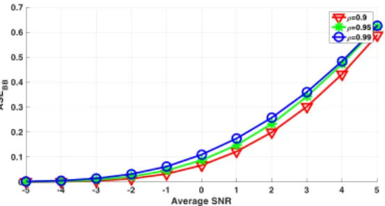
In Fig. 6, 𝐴𝑆𝐸𝐵𝐵 is plotted versus average SNR of the link for three different values of 𝜌. It is assumed that 𝜇 = 1 and the first set of modes are utilized with 𝐵0= 10−5.
Noting figures 4, 5 and 6 the following noticeable observations are made:
The ASE is considerably improved with the proposed optimum mode selection algorithm compared to the case in which modes are selected from equal probability intervals. The mentioned bench mark is the most intuitive scenario however with low average SNR, it may not be possible to find proper modes in the intervals, although with powerful LDPC codes.
The ASE by the proposed scheme is considerably improved in comparison to the case in which modes set is fixed by changing the link’s characteristics.
IV. CONCLUSION
A new algorithm was designed for optimal selection of modes set for an adaptive modulation and coding transmission, while, imperfect channel state information is available. The selection was done based on the statistics of SNR and the BER constraint. The selected modes set is used after codifying an agreement between the receiver and the transmitter at the beginning of the communication. After determining the modes set, only the index of appropriate mode is computed and sent back to the transmitter. Numerical evaluations indicate that with the proposed algorithm the performance may be considerably improved in comparison with other benchmarks, meanwhile imperfect CSI does not cause to restrict this algorithm to find best set of modes.
APPENDIX I
To proof that 𝐴𝑆𝐸 in 8 is a concave function of the thresholds, it should be shown that determinate of Hessian matrix (𝐻̃𝑀×𝑀) always is non-positive. We have:
𝐻̃𝑀×𝑀=
[
ℎ11 ℎ12 … ℎ1,𝑀
ℎ21 ℎ22 . . . ℎ2,𝑀
… ℎ𝑀,1
… ℎ𝑀,2
… …
… ℎ𝑀,𝑀
] , ℎ𝑖,𝑗= 𝜕2𝐴𝑆𝐸
𝜕𝛾𝑖𝜕𝛾𝑗 12
where the elements of this matrix (ℎ𝑖,𝑗) are obtained by 8 and 9 as follows,
ℎ𝑖,𝑗=
{
𝐴𝑓𝛾(𝛾𝑗) 𝛾𝑖+𝐵𝐶
𝑖 = 𝑗 − 1
𝐴𝑓𝛾(𝛾𝑖)
𝛾𝑗+𝐶𝐵 𝑖 = 𝑗 + 1
0 other wise
, 1 ≤ 𝑖, 𝑗 ≤ 𝑀 13
It can be shown easily that |𝐻̃𝑀×𝑀| is always non-positive.
REFERENCES
[1] S. T. Chung and A. J. Goldsmith, “Degrees of freedom in adaptive modulation: A unified view,” IEEE Trans. Commun., vol. 49, no. 9, pp. 1561–1571, Sep. 2001.
[2] Part 11: Wireless LAN Medium Access Control (MAC) and Physical Layer (PHY) Specifications, IEEE Std. 802.11a-1999, 1999.
[3] Digital Video Broadcasting (DVB) Second generation framing structure for broadband satellite applications, EN 302 307 V1.1.1, 2005.
[4] M. Taki, M. Sadegi, “Joint Relay Selection and Adaption of Modulation, Coding and Transmit Power for Spectral Efficiency Optimization in Amplify- Forward Relay Network”, IET Transaction on communications, Vol. 8, No. 11, pp. 1955-1964, 2014.
[5] M. Taki, F. Lahouti, “Spectral Efficiency Optimization for an Interfering Cognitive Radio with Adaptive Modulation and Coding”, IEEE Transaction on wireless communications, Vol. 10, No. 9, pp. 2929-2939, 2011.
[6] J. W. Hwang, and M. Shikh-Bahaei, “Packet error rate-based adaptive rate optimisation with selective-repeat automatic repeat request for convolutionally-coded M-ary quadrature amplitude modulation systems”, Communications, IET, Vol. 8, No. 6, pp. 878-884, 2014.
[7] J. Tang and X. Zhang, “Quality-of-service driven power and rate adaptation over wireless links,” IEEE Trans. on Wireless Commun., vol. 6, no. 8, pp. 3058–3068, Aug. 2007.
[8] A. Olfat and M. Shikh-Bahaei, “Optimum power and rate adaptation for MQAM in Rayleigh flat fading with imperfect channel estimation,” IEEE Trans. Veh. Technol., vol. 57, no. 4, pp. 2622–2627, Jul. 2008.
[9] Qian, Chuyi, Yi Ma, and Rahim Tafazolli, “Adaptive modulation for cooperative communications with noisy feedback,” Wireless Communications and Mobile Computing Conference (IWCMC), 2011 7th International. IEEE, 2011. [10] W.-L. Li, Y. J. Zhang, A.-C. So, and M. Win, “Slow adaptive
OFDMA systems through chance constrained programming, ”IEEE Trans. Signal Process., vol. 58, no. 7, pp. 3858–3869, Jul. 2010.
[11] L. Toni and A. Conti, “Does fast adaptive modulation always outperform slow adaptive modulation,” IEEE Trans. Wireless Commun., vol. 10, no. 5, pp. 1504–1513, May 2011. [12] L. Musavian, T. Le-Ngoc, “QoS-based power allocation for
cognitive radios with AMC and ARQ in Nakagami‐m fading channels,” Transactions on Emerging Telecommunications Technologies, vol. 27, pp. 266-277, February 2014.
[13] N. C. Beaulieu, G. Farhadi, and Y. Chen, “Amplify-and-forward multihop relaying with adaptive M-QAM in Nakagami-m fading,” in Proc. IEEE Global Telecommun. Conf., Dec. 2011.
[14] M. Taki, R. Mahin Zaeem, and M. Heshmati. “Throughput optimized error-free transmission using optimum combination of AMC and ARQ based on imperfect CSI.” Information and Communication Technology Research (ICTRC), 2015 International Conference on. IEEE, May 2015, pp. 182-185.
[15] M. Taki, M. Rezaiee, M. Guillaud, “Adaptive Modulation and Coding for Interference Alignment with Imperfect CSIT”, IEEE Transaction on wireless communications, Vol. 13, No. 9, pp. 5264-5273, 2014.
[16] S. Lin and D. J. Costello, “Error Control Coding: Fundamentals and Applications,” Englewood Cliffs, NJ: Prentice-Hall, 1983. [17] Rao, S. Singiresu, and S. S. Rao Engineering optimization:
theory and practice. John Wiley Sons, 2009.
[18] Y. Yasuda, et. al, “High rate punctured convolutional codes for soft decision Viterbi decoding, ” IEEE Transactions on Communications, vol. COM-32, No. 3, pp. 315–319, 1984.
Fig. 1. 𝑅̂𝑛 versus 𝑔𝐵0( 𝑅̂𝑛), 1 ≤ 𝑛 ≤ 𝑁 = 72; for the first set
of modes
Fig. 2. 𝑅̂𝑛 versus 𝑔𝐵0( 𝑅̂𝑛), 1 ≤ 𝑛 ≤ 𝑁 = 33; for the second
set of modes
Fig. 3. Comparison of ASE versus number of modes for different scenarios (8, 10 and 11); The second set of modes are utilized, Nakagami-m fading model with 𝜇 = 4 and average SNR of 0𝑑𝐵; 𝜌 = 0.95 and 𝐵0= 10−5
Fig. 4. Normalized 𝐴𝑆𝐸 (ASE divided to 𝐴𝑆𝐸𝑜𝑝𝑡_𝑞𝑢𝑎𝑛𝑡 in 11) versus the average SNR, comparison of different scenarios; first set of modes; Nakagami-m fading model with
𝜇 = 1; 𝐵0= 10−4; 𝜌 = 0.95 and number of modes 𝑀 = 3
Fig. 5. 𝐴𝑆𝐸 versus the number of modes for different order of Nakagami-m fading 𝜇 = 1 𝑜𝑟 3; optimum mode selection in comparison with selection from equal probability intervals; first set of modes; 𝜌 = 0.99 and 𝐵0= 10−4.
Fig. 6. 𝐴𝑆𝐸𝐵𝐵 for three different values of 𝜌; first set of modes, 𝜇 = 1 and 𝐵0= 10−5
Mehrdad Taki received the B.S.
degree from the University of Tehran, Tehran, Iran, in 2002, the M.S. degree from Iran University of Science and Technology, Tehran, in 2005, and the Ph.D. degree from the University of Tehran, in 2011, all in electrical communication engineering. He is currently an Assistant Professor at the University of Qom, Qom, Iran. His current research interests include communication theory, wireless multimedia communication, video and image processing and stochastic programming.
Reza Mahin Zaeem was born in 1989. He received his Bachelor and Master in Electrical engineering from Islamic Azad University Karaj branc and University of Isfahan in 2012 and 2015, respectively. From 2015, he focuses on "In-Bulding Solutions
and Telecommunication
Infrastructures". His research interests include “Cross Layer Design, Linear Block Codes, Multi-Hop Relaying and MIMO systems”.