Training Arti
fi
cial Neural Networks:
Backpropagation via Nonlinear
Optimization
Jadranka Skorin-Kapov
1and K. Wendy Tang
21W.A. Harriman School for Management and Policy, State University of New York at Stony Brook, Stony Brook, USA 2Department of Electrical and Computer Engineering, State University of New York at Stony Brook, Stony Brook, USA
In this paper we explore different strategies to guide backpropagation algorithm used for training artificial neural networks. Two different variants of steepest descent-based backpropagation algorithm, and four dif-ferent variants of conjugate gradient algorithm are tested. The variants differ whether or not the time component is used, and whether or not additional gradient information is utilized during one-dimensional optimization. Testing is performed on randomly generated data as well as on some benchmark data regarding energy prediction. Based on our test results, it appears that the most promissing backpropagation strategy is to initially use steepest descent algorithm, and then continue with con-jugate gradient algorithm. The backpropagation through time strategy combined with conjugate gradients appears to be promissing as well.
Keywords: Artificial intelligence: backpropagation in neural networks, Nonlinear unconstrained programming: conjugate gradient method, steepest descent method
1. Introduction
One of the key issues when designing a par-ticular neural network is to calculate proper weights for neuronal activities. These are ob-tained from the training process applied to the given neural network. To that end, a training sample is provided, i.e. a sample of observa-tions consisting of inputs and their respective outputs. The observations are ‘fed’ to the net-work. In the training process the algorithm is used to calculate neuronal weights, so that the squared error between the calculated outputs and observed outputs from the training set is minimized. Such an approach gives rise to an unconstrained nonlinear minimization problem, which can be solved with a number of existing
methods. First order methods (such as
steep-est descent) sometimes lack fast convergence,
while second order methods (e.g. Newton’s
method) are computationally expensive 3, 4].
Johansson et al. 6]compare the use of
conju-gate gradient method in backpropagation with conventional backpropagation and steepest de-scent.(Conventional backpropagation refers to
steepest descent with constant learning rate, i.e. step size, instead of using line search to get step sizes for each iteration.) For the data tested
(three, four and five bit parity problems) the
authors report that conjugate gradient backprop-agation is much faster than conventional back-propagation. Mangasarian7]discusses the role
of mathematical programming, particularly lin-ear programming, in training neural networks, and demonstrates it on the system developed for breast cancer diagnosis.
Our study is motivated by neuro-control appli-cations in complex systems. As neural networks are originally inspired by the human brain, one of the ultimate goals of neural network research is to demonstrate possible “brain-like" intelli-gence in the control area15]. To this end,
Wer-bos has summarized the pros and cons of five major neuro-control strategies 16]. Of these
strategies, backpropagation of utility is capable of controlling a complex system to maximize a utility function. Tang and Pingle 11] have
However, the success of the algorithm hinges upon sufficient training of a neural network to emulate the dynamic system.
In this paper we show that combined steepest descent and conjugate gradient methods offer advantages regarding neural network training over both of those methods if taken separately. Our task is to decide on the most appropriate strategy utilizing a combination of steepest de-scent and conjugate gradients for solving some randomly generated, as well as some bench-mark data sets. In addition, we stress the im-portance of the above neural network training in a more complex system with application to neuro-control(e.g. robotic arm training).
The neural network training process is undoubtly one of the most challenging tasks when design-ing a neural network. Moreover, it is a nat-ural task for utilizing mathematical program-ming theory. In the sequel we elaborate further on this issue. Specifically, the process of ob-taining appropriate weights in a neural network design utilizes two sets of equations. First, the feedforward equationsare used to calculate the error function, i.e. the objective function to be minimized. This is a differentiable function. The feedback equations are next used to cal-culate the gradient vector, which is then used for defining search directions in order to mini-mize the error function. Well known methods from unconstrained nonlinear minimization of differentiable functions include steepest descent and conjugate gradient methods. An efficient method should be stable and should converge fast. The gradient direction is the direction of steepest descent. The conjugate directions in-troduce certain modifications in directions in order to speed up the convergence. (In
partic-ular, for a positive definite quadratic function ofnvariables, the convergence is achieved inn iterations.) In Section 2 we outline the
back-propagation algorithm. Section 3 presents our computational results. Finally, in Section 4 the conclusions and directions for further research are presented. The Appendix contains our com-putational results in tabular form.
2. Backpropagation Algorithm
The backpropagation algorithm for training neu-ral networks has been discussed in many papers
(e.g. in Werbos13]). The work in this paper
is a continuation of the work by Tang and Chen
10]where the authors compare basic
backprop-agation versus backpropbackprop-agation through time al-gorithms. They presented a set of feedforward and feedback equations used for training neural networks. For completeness we briefly restate them.
Let us assume a neural network architecture with two hidden layers and withminputs,n out-puts,H1 hidden nodes in the first hidden layer, andH2 hidden nodes in the second hidden layer. For each input node there is a training sample consisting of T (m + n)-dimensional vectors
(Xi(t) Yj(t)), where (Xi(t) i = 1 ::: m) is a
set of input values, and(Yj(t) j=1 ::: n)the
set of corresponding outputs. The basic idea is to train the network so that given a set of inputs Xi(t), i = 1 ::: m, the network produces the
set of outputs Yj(t), j = 1 ::: n, which is as
close as possible to its desired(or true) set of
outputs Yj(t), j = 1 ::: n. In the sequel, Wl
will denote the weight of network nodel, and s(z) = 1=(1+e
;z
) will denote the sigmoidal
transferfunction.
In the basic backpropagation algorithm, the feedforward equations used to calculate the er-ror function are given as follows14]:
hid1h1(t)=
m
X
i=1
W(h1;1)m+i Xi (t)
h1=1 ::: H1; t=1 ::: T (1)
z1h1(t)=s(hid1h1(t))
h1=1 ::: H1; t=1 ::: T (2)
hid2h2(t)=
H1
X
h1=1
WH1m+(h2;1)H1+h1 z1h1 (t)
h2=1 ::: H2; t=1 ::: T (3)
z2h2(t)=s(hid2h2(t))
h2=1 ::: H2; t=1 ::: T (4)
netj(t)=
H2
X
h2=1
WH1m+H1H2+(j;1)H2+h2 z2h2 (t)
j=1 ::: n; t=1 ::: T (5)
Yj(t)=s(netj(t))
j=1 ::: n; t=1 ::: T (6)
E=
T
X
t=1
E(t)=
T
X
t=1
n
X
j=1
0:5Yj(t);Yj(t)]
2
(7)
This is an unconstrained minimization prob-lem with differentiable function of weightsWl,
l=1 ::: H1 m+H1 H2+H2 n.
There-fore, in order to minimize it we need to calculate its gradient, i.e. grad Wl. This is achieved via feedback equations as follows. For thetransfer function s(z) = 1=(1+e
;z
), its derivative is
s0
(z)=s(z) (1;s(z)). Then,
grad netj(t)=(Yi(t);Yi(t)) s 0
(netj(t))
j=1 ::: n (8)
grad hid2h2(t)=
n
X
j=1
W(H1m+H1H2+(j;1)H2+h2
grad netj(t)] s 0
(hid2h2(t))
j=1 ::: n; t=1 ::: T (9)
grad hid1h1(t)=
H2
X
h2=1
WH1m+(h2;1)H1+h1
grad hid2h2(t)] s 0
(hid1h1(t))
h1=1 ::: H1; t=1 ::: T (10)
grad W(h1;1)m+i =
T
X
t=1
grad hid1h1(t) Xi(t)
h1=1 ::: H1; i=1 ::: m (11)
grad WH1m+(h2;1)H2+h1
=
T
X
t=1
grad hid2h2(t) s 0
(hid1h1(t))
h1=1 ::: h1; h2 =1 ::: h2 (12)
grad Wh1m+H1H2+(j;1)H2+h2
=
T
X
t=1
grad netj(t) s 0
(hid2h2(t))
h2=1 ::: H2; j=1 ::: n (13)
New weights are iteratively obtained as
Wnew
l =Wl;αl grad Wl
l=1 ::: H1 m+H1 H2+H2 n (14)
where αl is the learning rate. In this paper,
we use Jacobs’ Delta-Bar-Delta5]method for
updatingαl.
In order to enhance the basic backpropagation algorithm, Werbos13, 14]proposed the
back-propagation through time algorithm, which in-corporates limited memory from past time peri-ods. This is achieved via a second set of weights W0
, added to each hidden and output node. (See,
for example, Tang and Chen10])
2.1. Steepest Descent Versus Conjugate Gradient Algorithm
When minimizing an objective function, we want to find directions of steepest decrease in functional values. One can pose the follow-ing problem: For all directions y with some bounded length, find the direction of steepest descent in functional value off at a given point x0, for which
rf(x
0
) 6= 0. This is a nonlinear
problem and its solution states that the steepest descent is the direction of the negative gradi-ent. The steepest descent method is an iterative method moving from an initial point through a sequence of points in directions of negative gradients. At each iteration the step size is either obtained via one-dimensional optimiza-tion, or it is given in advance as a parameter
(in the neural network vocabulary, this strategy
corresponds to the basic backpropagation). For
a quadratic function, a convergence of steepest descent method depends highly on the condition number of the quadratic matrix, which in turn depends on the difference between the smallest and largest eigenvalue of the matrix: if there is a big difference, the contours of the quadratic function are cigar shaped elipsoids around the minimal point. This results in poorer conver-gence, especially closer to the minimal point.
(For a non-quadratic function the idea is to use
the Hessian of the objective at the solution point as if it were the quadratic matrix of a quadratic problem.)
Tang and Chen 10] studied backpropagation
between steepest descent and conjugate gradi-ent. To that end, we briefly summarize the main idea behind a conjugate gradient algorithm. Suppose we have f : Rn
7! R, where f is
a twice continuously differentiable function. When minimizing a function, we want to have a descent method (like the steepest descent),
but also a method that converges fast, say in a finite number of steps (unlike the steepest
de-scent), when applied to the quadratic function.
(It is reasonable to assume that a nonlinear
func-tion can be reasonably well approximated by a quadratic function in the neighborhood of a min-imal point.) The method of conjugate gradients
combines descent property and a finite conver-gence for the quadratic case. The method pro-ceeds iteratively as follows. Start withx0. At iteration k let the new point xk be obtained as
xk
= x
k;1 +αkz
k, where zk is the direction of
the move, andαkis the step size. For a given
di-rectionzk,α
kis obtained by minimizingf along
zk. Namely, let F
(α
k
) = f(x
k;1 +αkz
k
), and
letα
k denote the minimum ofF. Therefore
@F(α
k) @αk
=z
kT
rf(x
k;1
+α
kzk)
=z
kT
rf(x
k
)=0: (15)
In the case of a quadratic function, we can get an explicit representation of α
k. Let f(x) =
a+b
Tx
+
1
2xTQx, whereQis annnpositive
definite matrix. Then,rf(x
k
)=b
T
+Qx
k, so
α
k =;
zkTrf(x
k;1 )
zkT
Qzk : (16)
For a method to be descent, we need to have f(x
k;1
) ; f(x
k
) > 0, which by rearranging
terms and using(16)translates toz
kT
rf(x
k;1 )
6= 0. (I.e. for having a descent method, the
only requirement is that the direction in k-th iteration, zk, is not orthogonal to the gradient at preceding point, rf(x
k;1
). The next
ques-tion is: which direcques-tions are good with respect to convergence? The conjugate directions are defined as follows.
DefinitionTwo vectorsx 2R
n y
2R
nare said
to be conjugate directions with respect to an nn symmetric positive definite matrix A if
xTAy
= 0. (IfA I, conjugate directions are
standard orthogonal directions.)
Conjugate gradientsare extensions of conjugate directions for differentiable functions. The con-jugate gradient algorithm due to Fletcher and Reeves2]runs as follows:
1. Selectx0 2R
n, the initial or starting solution.
2. Evaluaterf(x
0
), and letz
1
=;rf(x
0
).
3. Generate x1, x2,
:::, x
n by minimizing f
along the directions z1 z2 ::: z
n,
respec-tively, where xk+1
= x
k
+ α
k+1
zk+1, and α
k+1
minimizes f(x
k
+ αk +1z
k+1
). (It is
found, e.g., by line search). Define
zk+1
=;rf(x
k
)+
rf(x
k
)
T
rf(x
k
)
rf(x
k;1 )
T
rf(x
k;1 )
zk:
(17)
The first part ofzk+1
corresponds to steepest de-scent, and the second part is the “modification" introduced to speed up the convergence, based on conjugate directions.
Ifrf(x
k
)rf(x
k
) , where is a small
tol-erance, the algorithm will stop, since it will as-sumerf(x
k
)=0. Otherwise, for quadraticf it
will stop afterniterations. If the function is not quadratic, the convergence innsteps is not guar-anteed. Polak-Ribi`ere-Polyak(see e.g. Avriel
1])proposed the version of conjugate gradient
algorithm wherezk+1
= ;rf(x
k
)+βkz
k k
=
1 2 ::and
βk =
rf(x
k
);rf(x
k;1 )]
T
rf(x
k
)
rf(x
k;1 )
T
rf(x
k;1 )
: (18)
Global convergence holds if the method is peri-odically restarted. For example, if everynsteps we choosezk+1
= ;rf(z
k
) k = n 2n 3n ::: (which corresponds to the steepest descent
di-rection). The convergence of conjugate
gra-dient algorithm strongly depends on the initial point. If relatively ‘far away’ from the mini-mum, the approximation with a quadratic func-tion will not be accurate(which is a prerequisite
for the success of conjugate gradient strategy),
2.2. Conjugate Gradient Algorithm Applied to Backpropagation in Neural Networks
First, the feedforward equations are used to cal-culate the objective function (a differentiable
function of weights) to be minimized. Then,
the feedback equations lead to the gradient cal-culation. Those subroutines are used in the conjugate gradient algorithm employing Polak-Ribi`ere-Polyak(PRP)strategy.
One-dimensio-nal subproblems (to get the right step size in
each iteration) employ line search
minimiza-tion. One-dimensional minimization was per-formed using parabolic interpolation and Brent’s method(see, e.g. Vetterling et al. 12]). Brent’s
method can be implemented so that it optionally utilizes the derivative information available for one-dimensional problems. In the next section we compare different backpropagation strate-gies.
3. Computational Results
Our approach of combining steepest descent and conjugate gradients was first tested on randomly generated data for the sinus function.The net-work has one input node (m = 1), one
out-put node (n = 1), and 20 hidden nodes
ar-ranged in two hidden layers each having 10 nodes. We generated twenty pairs (T = 20)
of (Xi Yi = sin(Xi)) points and ‘fed’ it to the
network. By adjusting the weights, the task was to minimize the sum of squared errors between valuesYi(which the network would output)and
the true valuesYi. The program was written in
C and conjugate gradient routines from Vetter-ling et al. 12] were used. The testing was
performed on a Sun SPARC 2 workstation. The following versions of backpropagation stra-tegy were tested:
1. BBSD(Basic backpropagation with
steep-est descent);
2. BTSD (Backpropagation through time
with steepest descent);
3. BBCG (Basic backpropagation with
con-jugate gradients);
4. BTCG (Backpropagation through time
with conjugate gradients);
5. BBCGD(Basic backpropagation with
con-jugate gradients using derivatives for one-dimensional optimization);
6. BTCGD (Backpropagation through time
with conjugate gradients using derivatives for one-dimensional optimization);
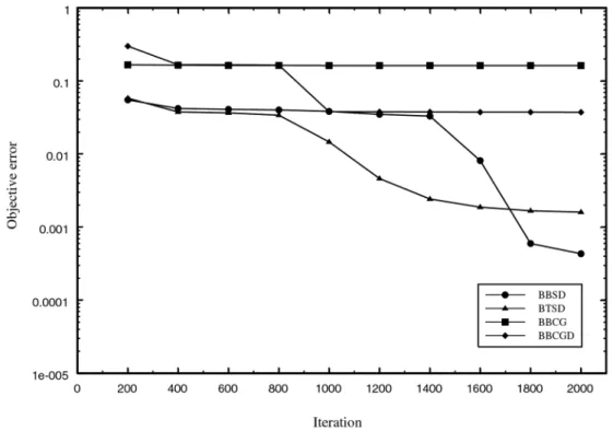
Fig. 2.Sine Data with Initial Weights after 2000 iteration of BBSD
BBSD and BTSD strategies were implemented using the same parameters, and delta-bar-delta rule as in Tang and Chen 10], so we will not
elaborate it further. In the BTSD algorithm, the time component was introduced after 100 iterations of BBSD, since the preliminary test-ing suggested that a delay in introductest-ing the time component results in more robust algo-rithm. (One iteration is one run over the
com-plete training set.)
We first ran 2000 iterations of each of the six dif-ferent strategies with randomly generated ini-tial weights (from the interval-0.1,0.1]). The
results are displayed in Figure 1. The ver-sions BTCG and BTCGD did not show con-vergence, hence we omitted them from display. The tabular displays accompanying the figures and showing computational times are presented in the Appendix.
If the criterionrf(x
k
)
T
rf(x
k
)is achieved,
the conjugate gradient algorithm stops. In our implementation = 10e;8 is the prescribed
tolerance. From the results, it appears that for a small number of iterations BBSD works better than other variants. (For an extended number
of iterations, BTSD outperforms the basic back-propagation, but the convergence overall is slow compared with the convergence obtained when
conjugate gradients are introduced.) Therefore,
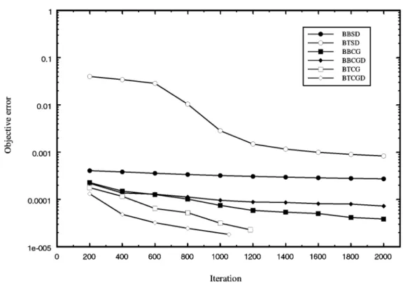
we decided to save in a file the weights obtained after 2000 iterations of BBSD, and use them as initial weights for the next round of testing. The results are displayed in Figure 2.
It is clear that, closer to the minimal point, the conjugate gradient strategy outperforms steep-est descent. It is more computationally inten-sive and requires more computing time, but the quality of the solution is one order of magnitude better.(An iteration of steepest descent requires
approximately 0.03 seconds, while an iteration of conjugate gradient method requires aproxi-mately 0.14 seconds.) The time component
in-troduced in backpropagation(backpropagation
through time)adds to solution quality, without
adding extra computational time. Utilization of derivatives in one-dimensional optimizations
(to obtain the best step size for moving along
the given direction)adds to expensiveness of the
algorithm, with marginal increase in the quality of the solution. (An iteration of conjugate
gra-dient with derivatives requires approximately 0.22 seconds.) On the basis of tested problems,
we therefore suggest to use the backpropagation through time conjugate gradient variant without derivatives, i.e. the version BTCG.
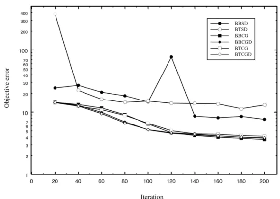
con-Fig. 3.Energy Prediction Data with Random Initial Weights
sumption in a building. It is part of a set of benchmark problems calledProben11for ANN learning 8]. In 8], Prechelt has included 15
benchmarking data sets from 12 different do-mains for ANN prediction and classification ap-plications. All but one of the database are data from real experiments. The building energy prediction database is one of the 15 datasets available.
This dataset was created based on a bench-mark problem of “The Great Energy Predictor Shootout – the first building data analysis and prediction problem" contest, organized in 1993 for theAmerican Society of Heating, Refrigerat-ing, and Air-Conditioning Engineers (ASHRSE) meeting in Denver, Colorado. The contest task was to predict the hourly consumption of elec-trical energy, hot water, and cold water based on the date, time of day, outside temperature, outside air humidity, solar radiation, and wind speed. Complete hourly data for 88 consecutive days were given for training.
The inputs to the neural networks including date, hour, weather-related parameters(
temper-ature, humidity, solar radiation and wind speed)
are encoded intom=14 parameters. There are
n = 3 outputs, the predicted hourly
consump-tion of electrical energy, hot water and cold wa-ter. The dataset consists of 88 days of hourly data. With the exception of the first day(resp.,
the last day), which only has 22 hours(resp., 18
hours)of data, all 24-hours are available, hence
a total ofT = 2104 samples. We initially ran
200 iterations of each of the algorithms, and the results are displayed in Figure 3.
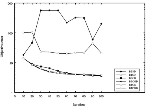
Backpropagation through time variants was in-troduced after 10 iterations. The iterations of steepest descent variants require less cpu time than the iterations of conjugate gradients ver-sions, but the convergence is slower. Based on the experience with randomly generatedsinus data, we saved the weights obtained after 200 it-erations of steepest descent algorithm BBSD. In the next round of testing, we ran 100 iterations of the algorithms starting with weights gener-ated from BBSD. The results are displayed in Figure 4, with better presentation of conjugate gradient variants repeated on a larger scale in Figure 5.
Similarly as in the case of randomly gener-ated data, it seems that the best strategy is to initially run backpropagation based on
Fig. 4.Energy Prediction Data with Initial Weights after 200 Iterations of BBSD
est descent, followed by the conjugate gradient version of backpropagation. In this way, com-parable results can be obtained much faster, due to ‘cheaper’steepest descent initial itera-tions. When the search comes closer to a minimal point, the conjugate gradient strategy provides much better convergence. The conju-gate gradient versions which employ derivatives for one-dimensional optimization (i.e.
algo-rithms BBCGD nd BTCGD) take much more
time than the basic conjugate gradient versions,
without improving the convergence. Regarding the convergence and speed, the backpropagation through time strategy combined with conjugate gradients provides similar results as the basic backpropagation. Hence, as in the case of ran-domly generated sinus data, it seems that the best backpropagation strategy is to initially run steepest descent, and then conjugate gradient algorithm.
In sum, from this study we confirmed our intu-ition that backpropagation with steepest decent
combined with conjugate gradient offers a pow-erful tool for training neural network.
4. Conclusions and Directions for Further Research
In this paper we studied the benefits of com-bining steepest descent and conjugate gradient algorithms as strategies to guide backpropaga-tion when training artificial neural networks. A neural network architecture with 2 hidden lay-ers(each with 10 hidden nodes)was trained on
randomly generated data for the sinus function,
as well as some benchmark data corresponding to energy prediction in applications from con-struction industry. The results suggest that with the combined strategy (start with steepest
de-scent, then switch to conjugate gradient)one is
able to achieve better accuracy in training than it would be achieved with separate strategies. The next task is to utilize the gained knowl-edge in a more complex learning systems, and in neural networks with more complex structure
(in terms of input, output, and hidden nodes).
From this study, we believe that steepest decent combined with conjugate gradient will offer a fast alternative in training such neural network.
4.1. Appendix: Tabulated Data
iter BBSD BTSD
obj. value time(sec) obj. value time(sec)
200 5.51918e-02 5.89 5.84926e-02 6.15
400 4.20617e-02 11.86 3.77279e-02 12.48
600 4.09564e-02 17.77 3.67574e-02 18.83
800 4.02316e-02 23.73 3.40680e-02 25.16
1000 3.84569e-02 29.70 1.47054e-02 31.48
1200 3.49867e-02 35.66 4.61972e-03 37.81
1400 3.31051e-02 41.63 2.43466e-03 44.11
1600 8.13298e-03 47.60 1.87984e-03 50.41
1800 5.96908e-04 53.57 1.67619e-03 56.68
2000 4.32921e-04 59.54 1.60801e-03 62.98
Table 1.Steepest descent strategy with random initial weights applied to randomly generated sinus data withm=1,
n=1,T=20
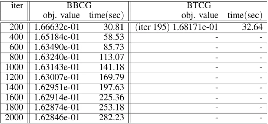
iter BBCG BTCG
obj. value time(sec) obj. value time(sec)
200 1.66632e-01 30.81 (iter 195)1.68171e-01 32.64
400 1.65184e-01 58.53 -
-600 1.63490e-01 85.73 -
-800 1.63240e-01 113.07 -
-1000 1.63143e-01 141.18 -
-1200 1.63007e-01 169.79 -
-1400 1.62951e-01 197.63 -
-1600 1.62914e-01 225.36 -
-1800 1.62874e-01 253.18 -
-2000 1.62846e-01 282.23 -
-Table 2.Conjugate gradient strategy with random initial weights applied to randomly generated sinus data with
iter BBCGD BTCGD
obj. value time(sec) obj. value time(sec)
200 2.99806e-01 45.91 (iter 136)2.80799e-01 41.37
400 1.67681e-01 90.59 -
-600 1.66815e-01 129.10 -
-800 1.64857e-01 169.27 -
-1000 3.79787e-02 210.03 -
-1200 3.78247e-02 247.07 -
-1400 3.76944e-02 283.25 -
-1600 3.75606e-02 320.24 -
-1800 3.74953e-02 356.84 -
-2000 3.72957e-02 393.61 -
-Table 3.Conjugate gradient using one-dimensional derivatives strategy with random initial weights applied to randomly generated sinus data withm=1,n=1,T =20
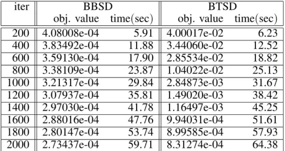
iter BBSD BTSD
obj. value time(sec) obj. value time(sec)
200 4.08008e-04 5.91 4.00017e-02 6.23
400 3.83492e-04 11.88 3.44060e-02 12.52
600 3.59130e-04 17.90 2.85534e-02 18.82
800 3.38109e-04 23.87 1.04022e-02 25.13
1000 3.21317e-04 29.84 2.84873e-03 31.67
1200 3.07937e-04 35.81 1.49020e-03 38.42
1400 2.97030e-04 41.78 1.16497e-03 45.25
1600 2.88016e-04 47.76 9.94031e-04 51.61
1800 2.80147e-04 53.74 8.99585e-04 57.93
2000 2.73437e-04 59.71 8.31274e-04 64.38
Table 4.Steepest descent strategy with initial weights obtained after 2000 iterations of BBSD algorithm, applied to randomly generated sinus data withm=1,n=1,T =20
iter BBCG BTCG
obj. value time(sec) obj. value time(sec)
200 2.28338e-04 27.77 1.77901e-04 30.38
400 1.50411e-04 54.82 1.16926e-04 58.28
600 1.27348e-04 81.87 6.44193e-05 85.64
800 1.02013e-04 109.61 5.26974e-05 112.97
1000 7.49826e-05 137.67 3.15274e-05 140.00
1200 5.86813e-05 165.36 (iter 1184)2.28776e-05 165.49
1400 5.37407e-05 191.59 -
-1600 5.04510e-05 218.55 -
-1800 4.16955e-05 246.16 -
-2000 3.87314e-05 273.78 -
iter BBCGD BTCGD
obj. value time(sec) obj. value time(sec)
200 2.20602e-04 38.33 1.32201e-04 51.55
400 1.37276e-04 78.95 4.85593e-05 118.15
600 1.29941e-04 119.54 3.23013e-05 175.94
800 1.12976e-04 157.41 2.45562e-05 232.77
1000 9.62196e-05 193.58 (iter 1053)1.82998e-05 308.86
1200 8.86204e-05 235.02 -
-1400 8.64339e-05 276.85 -
-1600 8.13103e-05 318.90 -
-1800 8.00507e-05 360.81 -
-2000 7.27481e-05 401.32 -
-Table 6.Conjugate gradient using one-dimensional derivatives strategy with initial weights obtained after 2000 iterations of BBSD algorithm, applied to randomly generated sinus data withm=1,n=1,T=20
iter BBSD BTSD
obj. value time(sec) obj. value time(sec)
20 24.519 93.39 380.130 96.83
40 27.016 186.93 22.356 194.59
60 20.885 280.61 16.098 295.65
80 18.322 374.43 14.355 393.37
100 14.581 468.30 15.069 491.11
120 77.067 562.20 13.921 588.94
140 8.628 656.1 13.785 687.00
160 8.120 750.03 13.569 785.08
180 8.536 844.12 11.382 883.06
200 7.667 939.17 13.050 981.01
Table 7.Steepest descent strategy with random initial weights applied to Energy prediction data withm=14,n=3,
T =2104
iter BBCG BTCG
obj. value time(sec) obj. value time(sec)
20 14.323 713.01 14.228 764.33
40 13.267 1371.64 12.443 1417.50
60 11.658 2045.48 10.924 2074.38
80 9.125 2699.71 8.844 2767.23
100 6.446 3340.48 6.619 3457.59
120 4.666 3961.86 5.022 4129.56
140 4.209 4577.71 4.483 5113.05
160 3.965 5165.32 4.403 5424.89
180 3.802 5729.07 4.199 6018.29
200 3.637 6316.07 4.095 6625.64
Table 8.Conjugate gradient strategy with random initial weights applied to Energy prediction data withm=14,
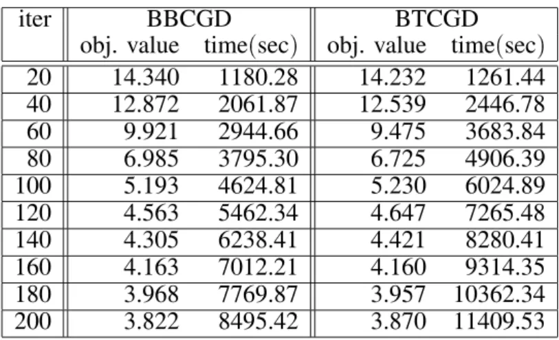
iter BBCGD BTCGD obj. value time(sec) obj. value time(sec)
20 14.340 1180.28 14.232 1261.44
40 12.872 2061.87 12.539 2446.78
60 9.921 2944.66 9.475 3683.84
80 6.985 3795.30 6.725 4906.39
100 5.193 4624.81 5.230 6024.89
120 4.563 5462.34 4.647 7265.48
140 4.305 6238.41 4.421 8280.41
160 4.163 7012.21 4.160 9314.35
180 3.968 7769.87 3.957 10362.34
200 3.822 8495.42 3.870 11409.53
Table 9. Conjugate gradient using one-dimensional derivatives strategy with random initial weights applied to Energy prediction data withm=14,n=3,T =2104
iter BBSD BTSD
obj. value time(sec) obj. value time(sec)
10 18.384 47.15 102.315 48.05
20 46.407 94.19 104.516 96.93
30 567.611 141.36 23.288 146.14
40 567.571 188.54 22.785 197.94
50 566.193 235.71 20.575 248.69
60 221.390 282.94 20.298 300.30
70 324.167 330.18 21.458 350.17
80 315.227 378.23 21.617 399.52
90 59.630 425.51 44.465 450.53
100 202.933 472.65 21.100 501.05
Table 10.Steepest descent strategy with initial weights obtained after 200 iterations of BBSD algorithm, applied to Energy Prediction data withm=14,n=3,T=2104
iter BBCG BTCG
obj. value time(sec) obj. value time(sec)
10 14.086 330.07 14.086 347.16
20 8.925 631.01 8.632 682.67
30 7.487 906.01 6.316 987.66
40 6.515 1184.68 5.073 1291.89
50 5.225 1474.37 4.739 1581.21
60 4.525 1748.22 4.321 1877.69
70 4.124 2017.45 4.214 2159.06
80 3.880 2301.37 4.139 2438.4
90 3.736 2576.11 3.967 2727.34
100 3.628 2852.75 3.804 3033.29
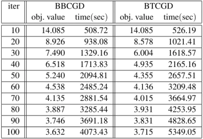
iter BBCGD BTCGD obj. value time(sec) obj. value time(sec)
10 14.085 508.72 14.085 526.19
20 8.926 938.08 8.578 1021.41
30 7.490 1329.16 6.004 1618.57
40 6.518 1713.83 4.935 2165.16
50 5.240 2094.81 4.355 2657.51
60 4.538 2485.24 4.136 3209.48
70 4.135 2881.54 4.015 3664.97
80 3.887 3285.44 3.931 4253.95
90 3.746 3691.18 3.831 4828.65
100 3.632 4073.43 3.715 5349.05
Table 12.Conjugate gradient using one-dimensional derivatives strategy with initial weights obtained after 200 iterations of BBSD algorithm, applied to Energy Prediction data withm=14,n=3,T=2104
Acknowledgement
The research of Jadranka Skorin-Kapov was partially supported by the NSF grants DDM-937417, SBR-9602021 and ANIR-9814014. The research of Wendy Tang was partially sup-ported by the NSF grants 9407363, ECS-9626655, ECS-9700313.
References
1] M. Avriel, 1976.Nonlinear Programming:
Analy-sis and Methods, Prentice-Hall Series in Automatic Computation.
2] R. Fletcher and BC.M. Reeves, 1964. “Function Minimization by Conjugate Gradients,"Computer Journal, 7,149-154.
3] S. Haykin, Neural Networks: A Comprehensive
Foundation, Second Edition, Prentice Hall, 1998.
4] J. Hertz, A. Krogh, and R.G. Palmer,Introduction
to the Theory of Neural Computation, Addison Wesley, 1990.
5] R. Jacobs, “Increased Rates of Convergence Through Learning Rate Adaptation", Neural Net-works, Vol.1, pp. 295-307, 1998.
6] E.M. Johansson, F.U. Dowla and D.M. Goodman, “Backpropagation Learning for Multi- Layer Feed-Forward neural Networks Using the Conjugate Gra-dient Method," Preprint, Lawrence Livermore Na-tional Laboratory, 1992.
7] O.L. Mangasarian, 1993. “Mathematical Program-ming in Neural Networks,"ORSA Journal on Com-puting, 5(4), pp. 349-360, 1993.
8] L. Prechelt, “PROBEN1 - A Set of Neural Network Benchmark Problems and Benchmarking Rules", Technical Report 21/94, Universitat Karlsruhe, Karlsruhe, Germany", September 1994.
9] J. Skorin-Kapov and W. Tang,“On Gradient Based Minimization Used in Backpropagation Method for Training Artificial Neural Networks," TR-770, Col-lege of Engineering and Applied Sciences, State University of New York at Stony Brook, 1999.
10] K.W. Tang and H.-J. Chen, “Comparing Basic Back-propagation and BackBack-propagation Through Time Algorithms" in the1995 World Congress on Neural Networks, Washington. D.C., July 17–21, 1995.
11] K.W. Tang and G. Pingle, “Exploring Neuro-Control with Backpropagation of Utility", Ohio Aerospace Institute Neural Network Symposium and Work-shop, Athens, Ohio, August 21–22, 1995, pp. 107–137.
12] W.T. Vetterling et al.,Numerical Recipes in C: the
art of scientific computing, Cambridge University Press, 1988.
13] P.J. Werbos, “Backpropagation Through Time: What It Does and How to Do It," Proceedings of the IEEE, 78(10), pp.1550-1560, 1990.
14] P.J. Werbos, The Roots of Backpropagation, John Wiley and Sons, Inc., New York, 1994.
15] P.J. Werbos and R. Santiago, “Brain-Like Intelli-gence in Artificial Models: How Can We Really Get There,"Above Threshold, International Neural Network Society, 2(2), pp.8-12, 1993.
Received:August, 1999
Revised:April, 2000
Accepted:May, 2000
Contact address:
Jadranka Skorin-Kapov W.A. Harriman School for Management and Policy State University of New York at Stony Brook Stony Brook, NY 11794-3775 phone:(631)632-7426
e-mail:[email protected] b.ed u
USA K. Wendy Tang Department of Electrical and Computer Engineering State University of New York at Stony Brook Stony Brook, NY 11794-2350 phone:(631)632-8404
e-mail:[email protected]
USA
JADRANKASKORIN-KAPOVreceived her B.Sc.(1977)and M Sc.(1983)
degrees in Applied Mathematics from the University of Zagreb, and her Ph.D.(1987)in Operations Research from the University of British
Columbia, Canada. She is currently a Professor at the W.A. Harriman School for Management and Policy, State University of New York at Stony Brook. Her research interests include combinatorial optimiza-tion, nonlinear programming, and development of solution procedures for difficult optimization problems arising in telecommunications, man-ufacturing, and facility layout and location. She has received five National Science Foundation grants and has published extensively, in-cluding articles in Mathematical Programming, Operations Research Letters, ORSA Journal on Computing, Computers and Operations Re-search, Discrete Applied Mathematics, Telecommunication Systems, Journal of Computing and Information Technology, European Journal of Operational research, and Annals of Operations Research.
K. WENDYTANGreceived her B.Sc.(1986), M Sc.(1988), and Ph.D.
(1991)degrees in Electrical Engineering from the University of
Roches-ter in RochesRoches-ter, New York. She is currently an Associate Professor at the Department of Electrical and Computer Engineering at the State University of New York at Stony Brook. Her research interests include artificial neural networks and communication networks. She is a recip-ient of the IEEE Third Millennium Award(2000), the IEEE Region 1
Award(1998), and the IEEE RAB Achievement Award(1998). She has