Issam Al-Azzoni
College of Engineering, Al Ain University of Science and Technology, Al Ain, United Arab Emirates
An Improved Coloured Petri Net Model
for Software Component Allocation on
Heterogeneous Embedded Systems
We extend an approach to component allocation on heterogeneous embedded systems using Coloured Petri Nets (CPNs). We improve the CPN model for the embedded systems and outline a technique that exploits CPN Tools, a well-known CPN tool, to ef-ficiently analyze embedded system's state space and find optimal allocations. The approach is model-based and represents an advancement towards a model-driv-en model-driv-engineering view of the componmodel-driv-ent allocation problem. We incorporate communication costs be-tween components by extending the CPN formalism with a non-trivial technique to analyze the generated state space. We also suggest a technique to improve the state space generation time by using the branch-ing options supported in CPN Tools. In the evaluation, we demonstrate that this technique significantly cuts down the size of the generated state space and thereby reduces the runtime of state space generation and thus the time to find an optimal allocation.
ACM CCS (2012) Classification: Software and its
en-gineering → Software notations and tools → Context specific languages → Domain specific languages Computer systems organization → Embedded and cy-ber-physical systems → Embedded systems → Em-bedded software
Keywords: component allocation, coloured Petri Nets,
model-driven engineering, embedded systems, hetero-geneous systems
1. Introduction and Related Work
Designers of embedded systems today face new challenges due to the high heterogeneity that characterizes such systems [1]. An em-bedded system may consist of several types of processors (or computational units) varying in
terms of their performance, including Central Processing units (CPUs), Graphical Process-ing Units (GPUs), and Field Programmable Gate Arrays (FPGAs). Also, the software com-ponents which need to be allocated on top of the hardware computational units may differ in terms of their resource usage. Such kind of het-erogeneity presents a challenge to the designers when deciding about the placement of software components on top of the computational units [2].
The component allocation problem finds op-timal allocations or mappings of the software components to the computational units [3]. While several allocations can be functionally correct in terms of being feasible, one or more of these allocations can have better non-func-tional (quality) aspects than the remaining allo-cations. Finding the allocation that is function-ally correct and that maximizes a certain quality metric is at the heart of solution methods to the component allocation problem. The component allocation problem can be formulated as an integer linear programming problem and thus there are several solution methods in mathe-matical optimization to the component alloca-tion problem [4], [5].
rich set of supporting theory and automated tools for model analysis [7], [8]. In this paper, we extend the work presented in [6]. The new contributions of this paper are summarized as follows:
1. We incorporate the communication costs between software components in the prob-lem definition and the CPN model. In [6], the communication costs were not included. 2. We make several changes to the CPN mod-el in order to improve the state space gen-eration time.
3. We modify the CPN model and the CPN ML queries to incorporate the communica-tion costs. This is not trivial, since it can-not be directly accounted for in the CPN body similar to the non-communication resource costs.
4. We run several more experiments to veri-fy the optimal allocations found using our CPN approach.
5. We suggest a technique to scale the CPN approach to larger systems by using the branching options in CPN ML state space generation tool. This is presented in Sub-section 3.3.
The use of a model-based approach has several benefits. For example, the same CPN model can be used to address the optimal allocations for other types of non-functional analysis, includ-ing security and dependability. CPNs have been applied extensively in analyzing non-function-al aspects of systems [9], [10]. Furthermore, models of the embedded system in different notations can be automatically transformed into equivalent CPN models. Thus, the main con-tribution of devising a CPN model to address the component allocation problem in heteroge-neous embedded systems is the application of a model-driven engineering (MDE) approach to the problem.
MDE advocates the use of models in systems analysis and design [11], [12], [13]. The use of models permits various types of analysis to be performed on the models before the actual sys-tem is implemented. This can be done at a high level of abstraction and in an automated fashion. In [14], the authors propose an approach for the automatic transformation from an Ecore-based model of a component allocation problem into
an equivalent CPN model. The resulting CPN model can be analyzed using the method pre-sented in this paper. This allows to identify a component allocation problem and to solve it without having to know about CPNs.
The authors of [3] apply a genetic algorithm to find optimal solutions to the component al-location problem. Our model that defines the component allocation problem is based on the model presented in [3]. The authors also apply analytical hierarchical process to calculate the trade-off vector. Genetic algorithms usually find good solutions; however, generally speak-ing, there is no guarantee that these solutions are the optimal solutions. A prototype tool that implements the genetic algorithm is presented in [15]. The tool is named SCALL (Software Component ALLocator for Heterogeneous Embedded Systems). SCALL is developed as an Eclipse plugin utilizing Eclipse Modeling Framework (EMF) and Graphical Modeling Project (GMP). SCALL is based on using a metamodel for the software component alloca-tion problem specified in Ecore notaalloca-tion. The user of SCALL can create a model for a soft-ware component allocation problem in a drag-and-drop fashion from a palette. SCALL then returns an optimal allocation computed using the genetic algorithm presented in [3].
A model-driven engineering approach for com-ponent allocation is presented in [16]. The ap-proach allows to specify allocation constrains in ASL (Allocation Specification Language) that uses OCL operations. Then, the feasible al-locations can be derived automatically without having to know how to encode and solve the allocation problem as an integer linear program (ILP). This is achieved by using model-to-mod-el transformation that generates modmodel-to-mod-els for ILPs solvable by an ILP solver.
Another method for solving the component allocation problem is presented in [17]. The method uses branch-and-bound and forward checking mechanisms. The method was imple-mented in the Automatic Integration of Reus-able Embedded Software (AIRS) toolkit [18]. A generic framework aimed at finding the most appropriate deployment architecture (mapping of software components onto hardware resourc-es) for a distributed software system is present-ed in [2]. The framework formally defines the
tive networked embedded systems. The compo-nents communicate with each other via signals that can be periodic or sporadic. The presented algorithms minimize the total communication cost only and are based on graph partitioning theory. Our component model does not include signals. The CPN approach presented in this paper minimizes an objective cost function that includes multiple resources, including commu-nication.
The organization of the paper is as follows. In Section 2, we define the component allocation problem more formally. We illustrate our ap-proach in Section 3. In Section 4, we evaluate our CPN based approach. Section 5 concludes the paper and outlines future work.
2. Problem Definition
Consider a software system consisting of n
components. Every component needs to be as-signed to a computational unit on a hardware platform consisting of m computational units. The computational units offer a number of re-sources l (for example, computation, memory, and energy resources). Our model for the com-ponent allocation problem is based on [3]. The Component Resource Consumption Matrix
T = [tijk](n × m × l) defines the amount of
resourc-es each component requirresourc-es. The element tijk represents the necessary amount of the k-th re-source required by the i-th software component when allocated on the j-th computational unit. The Computational Unit Resource Capaci-ty Matrix R = [rjk](m × l) defines the amount of
resources that each computational unit can provide. The element rjk represents the k-th re-source capacity of a j-th computational unit. To incorporate the cost of communication be-tween the software components, we define two matrices. The first is the Communication Inten-sity Matrix K = [kij](n × n), where kij represents
the communication intensity between the i-th and j-th components. If the components i and
j are not communicating, then kij = 0. Also, no-tice that the matrix K is symmetric since the direction of communication is assumed to be not relevant. In addition, the diagonal elements of k are all equal to zero. The second matrix is the Platform Communication Cost Matrix component allocation problem and provides
a set of applicable algorithms for solving the problem. In addition, a tool suite is developed to enable the use of the proposed framework. The component allocation problem presented in this paper can be thought of as a particular instantiation of the framework. In addition, the CPN based approach can supplement the solu-tion algorithms presented in [2].
Another framework for modeling and analyz-ing the component allocation problem in het-erogeneous computing systems is presented in [19]. The framework is called LOSECO (an al-location of parallel software to heterogeneous computing platform framework). In LOSE-CO, the software execution units, which corre-spond to components in our model, can have precedence relationships amongst each other. Our component model assumes that the com-ponents are independent. The authors propose a partitioning based allocation heuristic which partitions the graph representing the software execution units and their dependencies into multiple smaller subgraphs. Subsequently, each subgraph is solved using heuristics such as ge-netic algorithms.
The authors of [1] present a formal model for allocation optimization of embedded systems which contain a mix of CPU and GPU process-ing nodes. The authors use mixed-integer non-linear programming as the optimization model. In addition, the authors translate the model into a solver using a standard format called MPS (Mathematical Programming System) that can be interpreted using most solvers. The authors make the observation that the mixed-integer nonlinear programming solvers do not scale well for medium and large size problems. Several approaches exist for component alloca-tion in real-time embedded systems [11], [20], [21], [22]. In real-time embedded systems, components (tasks) have additional attributes such as completion time, period, and deadline. The allocation problem for real-time embedded systems needs to ensure that tasks are com-pleted before their deadlines. Our CPN based approach uses a different component model which does not take these timing properties into account.
automo-rich set of supporting theory and automated tools for model analysis [7], [8]. In this paper, we extend the work presented in [6]. The new contributions of this paper are summarized as follows:
1. We incorporate the communication costs between software components in the prob-lem definition and the CPN model. In [6], the communication costs were not included. 2. We make several changes to the CPN mod-el in order to improve the state space gen-eration time.
3. We modify the CPN model and the CPN ML queries to incorporate the communica-tion costs. This is not trivial, since it can-not be directly accounted for in the CPN body similar to the non-communication resource costs.
4. We run several more experiments to veri-fy the optimal allocations found using our CPN approach.
5. We suggest a technique to scale the CPN approach to larger systems by using the branching options in CPN ML state space generation tool. This is presented in Sub-section 3.3.
The use of a model-based approach has several benefits. For example, the same CPN model can be used to address the optimal allocations for other types of non-functional analysis, includ-ing security and dependability. CPNs have been applied extensively in analyzing non-function-al aspects of systems [9], [10]. Furthermore, models of the embedded system in different notations can be automatically transformed into equivalent CPN models. Thus, the main con-tribution of devising a CPN model to address the component allocation problem in heteroge-neous embedded systems is the application of a model-driven engineering (MDE) approach to the problem.
MDE advocates the use of models in systems analysis and design [11], [12], [13]. The use of models permits various types of analysis to be performed on the models before the actual sys-tem is implemented. This can be done at a high level of abstraction and in an automated fashion. In [14], the authors propose an approach for the automatic transformation from an Ecore-based model of a component allocation problem into
an equivalent CPN model. The resulting CPN model can be analyzed using the method pre-sented in this paper. This allows to identify a component allocation problem and to solve it without having to know about CPNs.
The authors of [3] apply a genetic algorithm to find optimal solutions to the component al-location problem. Our model that defines the component allocation problem is based on the model presented in [3]. The authors also apply analytical hierarchical process to calculate the trade-off vector. Genetic algorithms usually find good solutions; however, generally speak-ing, there is no guarantee that these solutions are the optimal solutions. A prototype tool that implements the genetic algorithm is presented in [15]. The tool is named SCALL (Software Component ALLocator for Heterogeneous Embedded Systems). SCALL is developed as an Eclipse plugin utilizing Eclipse Modeling Framework (EMF) and Graphical Modeling Project (GMP). SCALL is based on using a metamodel for the software component alloca-tion problem specified in Ecore notaalloca-tion. The user of SCALL can create a model for a soft-ware component allocation problem in a drag-and-drop fashion from a palette. SCALL then returns an optimal allocation computed using the genetic algorithm presented in [3].
A model-driven engineering approach for com-ponent allocation is presented in [16]. The ap-proach allows to specify allocation constrains in ASL (Allocation Specification Language) that uses OCL operations. Then, the feasible al-locations can be derived automatically without having to know how to encode and solve the allocation problem as an integer linear program (ILP). This is achieved by using model-to-mod-el transformation that generates modmodel-to-mod-els for ILPs solvable by an ILP solver.
Another method for solving the component allocation problem is presented in [17]. The method uses branch-and-bound and forward checking mechanisms. The method was imple-mented in the Automatic Integration of Reus-able Embedded Software (AIRS) toolkit [18]. A generic framework aimed at finding the most appropriate deployment architecture (mapping of software components onto hardware resourc-es) for a distributed software system is present-ed in [2]. The framework formally defines the
tive networked embedded systems. The compo-nents communicate with each other via signals that can be periodic or sporadic. The presented algorithms minimize the total communication cost only and are based on graph partitioning theory. Our component model does not include signals. The CPN approach presented in this paper minimizes an objective cost function that includes multiple resources, including commu-nication.
The organization of the paper is as follows. In Section 2, we define the component allocation problem more formally. We illustrate our ap-proach in Section 3. In Section 4, we evaluate our CPN based approach. Section 5 concludes the paper and outlines future work.
2. Problem Definition
Consider a software system consisting of n
components. Every component needs to be as-signed to a computational unit on a hardware platform consisting of m computational units. The computational units offer a number of re-sources l (for example, computation, memory, and energy resources). Our model for the com-ponent allocation problem is based on [3]. The Component Resource Consumption Matrix
T = [tijk](n × m × l) defines the amount of
resourc-es each component requirresourc-es. The element tijk represents the necessary amount of the k-th re-source required by the i-th software component when allocated on the j-th computational unit. The Computational Unit Resource Capaci-ty Matrix R = [rjk](m × l) defines the amount of
resources that each computational unit can provide. The element rjk represents the k-th re-source capacity of a j-th computational unit. To incorporate the cost of communication be-tween the software components, we define two matrices. The first is the Communication Inten-sity Matrix K = [kij](n × n), where kij represents
the communication intensity between the i-th and j-th components. If the components i and
j are not communicating, then kij = 0. Also, no-tice that the matrix K is symmetric since the direction of communication is assumed to be not relevant. In addition, the diagonal elements of k are all equal to zero. The second matrix is the Platform Communication Cost Matrix component allocation problem and provides
a set of applicable algorithms for solving the problem. In addition, a tool suite is developed to enable the use of the proposed framework. The component allocation problem presented in this paper can be thought of as a particular instantiation of the framework. In addition, the CPN based approach can supplement the solu-tion algorithms presented in [2].
Another framework for modeling and analyz-ing the component allocation problem in het-erogeneous computing systems is presented in [19]. The framework is called LOSECO (an al-location of parallel software to heterogeneous computing platform framework). In LOSE-CO, the software execution units, which corre-spond to components in our model, can have precedence relationships amongst each other. Our component model assumes that the com-ponents are independent. The authors propose a partitioning based allocation heuristic which partitions the graph representing the software execution units and their dependencies into multiple smaller subgraphs. Subsequently, each subgraph is solved using heuristics such as ge-netic algorithms.
The authors of [1] present a formal model for allocation optimization of embedded systems which contain a mix of CPU and GPU process-ing nodes. The authors use mixed-integer non-linear programming as the optimization model. In addition, the authors translate the model into a solver using a standard format called MPS (Mathematical Programming System) that can be interpreted using most solvers. The authors make the observation that the mixed-integer nonlinear programming solvers do not scale well for medium and large size problems. Several approaches exist for component alloca-tion in real-time embedded systems [11], [20], [21], [22]. In real-time embedded systems, components (tasks) have additional attributes such as completion time, period, and deadline. The allocation problem for real-time embedded systems needs to ensure that tasks are com-pleted before their deadlines. Our CPN based approach uses a different component model which does not take these timing properties into account.
automo-C = [cij](m × m), where cij represents the
commu-nication cost between the i-th and j-th compu-tational units. For i = j, cij = 0. The inclusion of both matrices is necessary since the total com-munication cost depends on the comcom-munication intensity between the components in addition to the platform characteristics of the commu-nication channels connecting the computational units.
An allocation to the components maps each software component to one of the m compu-tational units. One or more components can be allocated on the same computational unit. From a mathematical viewpoint, an allocation represents a permutation with repetition which assigns one computational unit to each software component. Note that there are mn possible al-locations, which implies that the search space increases exponentially with the number of components and computational units.
Consider an allocation (p1, ..., pn), where com-ponent i is assigned to computational unit pi. An allocation is called feasible if the resources consumed by the software components allocat-ed to any computational unit do not exceallocat-ed the resource capacities that the computational unit provides. More formally, for any computational unit j, a feasible allocation satisfies the condi-tion:
i p j,
∑
i=( )
tipik ≤rjk (1)for all resources k.
In addition to satisfying (1), we might consider additional constraints that need to be satisfied by a feasible allocation. In this paper, we con-sider the system architectural constraint that in a feasible allocation a particular component should (or should not) be allocated to a set of computational units. There could be several of such architectural constraints that a feasible al-location needs to satisfy.
Given an allocation (p1, ..., pn), its cost can be computed using the following cost function:
1 1 i i j
l n
k ip k c ij p p
k i i j
w f t f k c
= = ≤
=
∑ ∑
+∑
(2) Here, fk represents a trade-off factor whose pur-pose is to specify the weights of each resource in the cost function. This allows to differentiate
the importance of different resources. Similar-ly, fc is the communication trade-off factor. The component allocation problem is to find an optimal allocation. An optimal allocation is a feasible allocation that has the smallest w
amongst all feasible allocations. Thus, the cho-sen allocation needs to satisfy (1) (in addition to possibly additional constraints) and has the smallest cost w which is defined by (2).
The component allocation problem can be
for-mulated as a 0 − 1 integer linear programming
problem which is NP-complete [24]. For exact solutions and small problem sizes (the problem size is based on the number of components and computational units), one can use traditional integer programming techniques. However, for large problem sizes, one needs to resort to heu-ristics which find good approximations through large space search methods.
3. Approach
In this section, we apply the CPN based ap-proach to solve a component allocation prob-lem using parameters of a realistic system bor-rowed from [3]. Subsection 3.1 gives a brief description of the system. In Subsection 3.2, we develop a CPN model of the system and in Subsection 3.3, we describe the generation and analysis of the state space using CPN Tools. Subsection 3.4 summarizes the approach.
3.1. Case Study
To demonstrate our approach, we borrow the same parameters used to develop a component allocation problem from [3]. The system con-sidered is a software system that handles and interprets vision data on an autonomous under-water vehicle (AUV), while simultaneously in-teracting with them in real time. That system is being developed as a part of RALF3 project [25].
The system consists of n = 11 components. These are: 1-UI User Interface, 2-CH Commu-nication Handler, 3-MP Message Parser, 4-MD Manual Drive, 5-MM Mission Manager, 6-MC Movement Control, 7-V Vision, 8-AC Actuator Control, 9-SI Sensors Layer 1, 10-S2 Sensors Layer 2, and 11-SF Stream Filtering
compo-nents. The hardware platform consists of m = 4 computational units. These are: 1-mCPU Mul-ticore CPU, 2-FPGA FPGA I, 3-FPGA FPGA II, and 4-GPU GPU. There are l = 3 resources: average execution time (measured in millisec-onds), memory (measured in megabytes), and average energy consumption (measured in mil-liamperes per hour).
10 90 90 55 50 20 20 72 30 20 20 72 10 40 40 72 20 40 40 72 20 50 50 55 90 20 20 15 20 10 10 70 20 10 10 70 20 15 15 70 90 10 10 33
48 256 256 128 128 256 256 148 64 256 256 148 48 168 168 148 64 168 168 148 64 168 168 64 168 128 128 64 148 96 96 148
48 32 32 148 48 32 32 148 168 64 64 96
(a) (b)
2 18 18 11 10 4 4 14 6 4 4 14 2 8 8 14 4 8 8 14 4 10 10 11 18 4 4 3
4 2 2 14 4 2 2 14 4 3 3 14 18 2 2 7
(c)
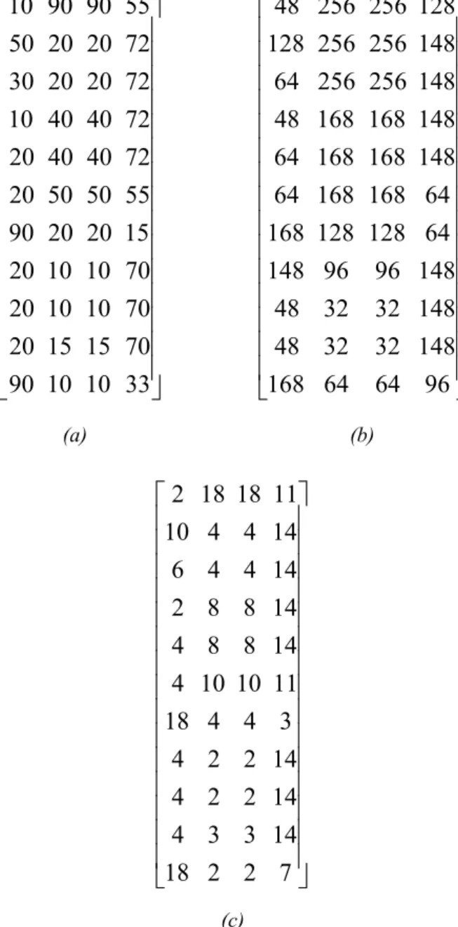
Figure 1 shows the component resource con-sumptions (i.e., the elements of the matrix T). Since T is three-dimensional (components, computational units, resources), we use three matrices to display three different resources
(i.e., the third dimension): a) average execution time, b) memory, and
c) average energy consumption.
The computational unit resource capacity ma-trix is given by:
100 256 50 150 640 25 150 640 25 100 256 15
R
=
0 1 0 0 0 0 0 0 0 0 0 1 0 5 0 3 0 0 0 0 0 0 0 5 0 5 3 0 0 0 0 0 0 0 0 5 0 0 1 7 3 0 0 0 0 3 3 0 0 9 9 3 0 0 0 0 0 0 1 9 0 0 0 7 7 0 0 0 0 7 9 0 0 0 0 0 7 0 0 0 3 3 0 0 0 0 0 0 0 0 0 0 0 7 0 0 0 0 0 0 0 0 0 0 7 0 0 0 0 0 0 0 0 0 0 0 7 0 0 0 0
Figure 2 shows the communication intensity matrix. The platform communication cost ma-trix is given by:
1 5 5 4 5 1 2 3 5 2 1 3 4 3 3 1
C
=
To compute the cost of an allocation in (2), we use the trade-off vector:
[
0.1557 0.0856 0.7095 0.0491]
F =
Here, the k-th element in vector F represents the trade-off factor fk. The trade-off factors are
Figure 1. The component resource consumptions.
C = [cij](m × m), where cij represents the
commu-nication cost between the i-th and j-th compu-tational units. For i = j, cij = 0. The inclusion of both matrices is necessary since the total com-munication cost depends on the comcom-munication intensity between the components in addition to the platform characteristics of the commu-nication channels connecting the computational units.
An allocation to the components maps each software component to one of the m compu-tational units. One or more components can be allocated on the same computational unit. From a mathematical viewpoint, an allocation represents a permutation with repetition which assigns one computational unit to each software component. Note that there are mn possible al-locations, which implies that the search space increases exponentially with the number of components and computational units.
Consider an allocation (p1, ..., pn), where com-ponent i is assigned to computational unit pi. An allocation is called feasible if the resources consumed by the software components allocat-ed to any computational unit do not exceallocat-ed the resource capacities that the computational unit provides. More formally, for any computational unit j, a feasible allocation satisfies the condi-tion:
i p j,
∑
i=( )
tipik ≤rjk (1)for all resources k.
In addition to satisfying (1), we might consider additional constraints that need to be satisfied by a feasible allocation. In this paper, we con-sider the system architectural constraint that in a feasible allocation a particular component should (or should not) be allocated to a set of computational units. There could be several of such architectural constraints that a feasible al-location needs to satisfy.
Given an allocation (p1, ..., pn), its cost can be computed using the following cost function:
1 1 i i j
l n
k ip k c ij p p
k i i j
w f t f k c
= = ≤
=
∑ ∑
+∑
(2) Here, fk represents a trade-off factor whose pur-pose is to specify the weights of each resource in the cost function. This allows to differentiate
the importance of different resources. Similar-ly, fc is the communication trade-off factor. The component allocation problem is to find an optimal allocation. An optimal allocation is a feasible allocation that has the smallest w
amongst all feasible allocations. Thus, the cho-sen allocation needs to satisfy (1) (in addition to possibly additional constraints) and has the smallest cost w which is defined by (2).
The component allocation problem can be
for-mulated as a 0 − 1 integer linear programming
problem which is NP-complete [24]. For exact solutions and small problem sizes (the problem size is based on the number of components and computational units), one can use traditional integer programming techniques. However, for large problem sizes, one needs to resort to heu-ristics which find good approximations through large space search methods.
3. Approach
In this section, we apply the CPN based ap-proach to solve a component allocation prob-lem using parameters of a realistic system bor-rowed from [3]. Subsection 3.1 gives a brief description of the system. In Subsection 3.2, we develop a CPN model of the system and in Subsection 3.3, we describe the generation and analysis of the state space using CPN Tools. Subsection 3.4 summarizes the approach.
3.1. Case Study
To demonstrate our approach, we borrow the same parameters used to develop a component allocation problem from [3]. The system con-sidered is a software system that handles and interprets vision data on an autonomous under-water vehicle (AUV), while simultaneously in-teracting with them in real time. That system is being developed as a part of RALF3 project [25].
The system consists of n = 11 components. These are: 1-UI User Interface, 2-CH Commu-nication Handler, 3-MP Message Parser, 4-MD Manual Drive, 5-MM Mission Manager, 6-MC Movement Control, 7-V Vision, 8-AC Actuator Control, 9-SI Sensors Layer 1, 10-S2 Sensors Layer 2, and 11-SF Stream Filtering
compo-nents. The hardware platform consists of m = 4 computational units. These are: 1-mCPU Mul-ticore CPU, 2-FPGA FPGA I, 3-FPGA FPGA II, and 4-GPU GPU. There are l = 3 resources: average execution time (measured in millisec-onds), memory (measured in megabytes), and average energy consumption (measured in mil-liamperes per hour).
10 90 90 55 50 20 20 72 30 20 20 72 10 40 40 72 20 40 40 72 20 50 50 55 90 20 20 15 20 10 10 70 20 10 10 70 20 15 15 70 90 10 10 33
48 256 256 128 128 256 256 148 64 256 256 148 48 168 168 148 64 168 168 148 64 168 168 64 168 128 128 64 148 96 96 148
48 32 32 148 48 32 32 148 168 64 64 96
(a) (b)
2 18 18 11 10 4 4 14 6 4 4 14 2 8 8 14 4 8 8 14 4 10 10 11 18 4 4 3
4 2 2 14 4 2 2 14 4 3 3 14 18 2 2 7
(c)
Figure 1 shows the component resource con-sumptions (i.e., the elements of the matrix T). Since T is three-dimensional (components, computational units, resources), we use three matrices to display three different resources
(i.e., the third dimension): a) average execution time, b) memory, and
c) average energy consumption.
The computational unit resource capacity ma-trix is given by:
100 256 50 150 640 25 150 640 25 100 256 15
R
=
0 1 0 0 0 0 0 0 0 0 0 1 0 5 0 3 0 0 0 0 0 0 0 5 0 5 3 0 0 0 0 0 0 0 0 5 0 0 1 7 3 0 0 0 0 3 3 0 0 9 9 3 0 0 0 0 0 0 1 9 0 0 0 7 7 0 0 0 0 7 9 0 0 0 0 0 7 0 0 0 3 3 0 0 0 0 0 0 0 0 0 0 0 7 0 0 0 0 0 0 0 0 0 0 7 0 0 0 0 0 0 0 0 0 0 0 7 0 0 0 0
Figure 2 shows the communication intensity matrix. The platform communication cost ma-trix is given by:
1 5 5 4 5 1 2 3 5 2 1 3 4 3 3 1
C
=
To compute the cost of an allocation in (2), we use the trade-off vector:
[
0.1557 0.0856 0.7095 0.0491]
F =
Here, the k-th element in vector F represents the trade-off factor fk. The trade-off factors are
Figure 1. The component resource consumptions.
computed using Analytic Hierarchy Process (AHP) [26]. The last element in F is the com-munication trade-off factor fc. The details are given in [3].
We will consider two additional constraints:
● Constraint I: Component 7-V should be allocated to 4-GPU.
● Constraint II: Component 4-MD should not be allocated to 1-mCPU.
3.2. The CPN Model
The CPN model is shown in Figure 3. The CPN contains four places. Here, we briefly describe each place. The place Components holds tokens which represent the components. The place
CompUnits holds tokens representing the com-putational units. Each token records the avail-able resources that the corresponding computa-tional unit currently has. The place Allocations
holds tokens which represent the allocations of components to computational units. The place
Cost holds a single token which records the total cost of the allocated components, exclud-ing the communication costs. There is only one transition in the CPN. Firing the transition allo-cate corresponds to assigning a component to one of the computational units.
The colour sets are defined as follows:
The colour set CompUnit is defined as the prod-uct of four integer colour sets. This is the colour set for the place CompUnits holding tokens that record the available resources in each computa-tional unit. In each such token, the colours are ordered as follows: the computational unit id, the available average execution time resource, the available memory resource, and the avail-able average energy consumption resource. The variables are declared as follows:
The variables c and cu hold the component and computational unit ids, respectively. The vari-able co holds the total cost of the allocated com-ponents, excluding the communication costs. The variables a_cpu, a_mem, and a_pwr hold
the available average execution time, memory, and average energy consumption resources, re-spectively.
To encode the component resource consump-tion matrix T, we define three two-dimension-al arrays: cp_cons, mem_cons, and ener_cons. This is done by using the function fromList de-fined on Array2 structures in SML library. For example, the array cpu_cons is defined using the following:
Components are allocated one by one, in or-der of their ids. This is valid, since the oror-der of assigning components to computational units does not matter with respect to the feasibility condition (see (1)). The assignment of compo-nents is controlled by the value of the token re-siding in place Components. Note that the com-ponent ids and the computational unit ids start from zero. Thus, for example, the component
with id = 0 corresponds to the component 1-UI and the computational unit with id = 0 corre-sponds to the computational unit 1-mCPU. The constraints are included in the CPN model by using the guard of transition allocate. For ex-ample, in Constraint I, Component 7-V should be allocated on 4-GPU. Thus, a feasible alloca-tion of components should satisfy the condialloca-tion that (c = 6) → (cu = 3) which is logically equiv-alent to ¬ (c = 6) ˅ (cu = 3). For Constraint II, Component 4-MD should not be allocated to 1-mCPU. Thus, a feasible allocation of com-ponents should also satisfy the condition that ¬ ((c = 3) ˄ (cu = 0)). Both conditions are added to the guard of transition allocate.
When a component is allocated to a computa-tional unit, the corresponding cost needs to be added to the total cost (the colour of the token in place Cost). This is modeled by using the arc from transition allocate to place Cost. Note the trade-off factors fk in the arc expression.
3.3. State Space Generation and Analysis
We use the state space tool of CPN Tools Ver-sion 4.0 to find an optimal component alloca-tion. CPN Tools Version 4.0 adds the support for real colorsets. Figure 4 shows the query functions used to generate and search through the state space. These queries are written in the CPN ML programming language (presented in Chapter 3 in [8]). For a given marking
repre-Figure 3. The CPN model for the system of the case study.
Components
INT 1`0
CompUnits CompUnit 1`(0,100,256,50)++1`(1,150,640,25)++ 1`(2,150,640,25)++1`(3,100,256,15)
Allocations
Allocation
Cost
REAL 1`0.0 allocate
[c<= 10 andalso a_cpu>= Array2.sub(cpu_cons,c,cu) andalso a_mem>= Array2.sub(mem_cons,c,cu) andalso
a_pwr>=Array2.sub(ener_cons,c,cu) andalso (not (c=6) orelse cu=3) andalso not (c=3 andalso cu=0)]
c (cu,a_cpu,a_mem,a_pwr)
(c,cu)
(cu,a_cpu-Array2.sub(cpu_cons,c,cu),a_mem-Array2.sub(mem_cons,c,cu),a_pwr-Array2.sub(ener_cons,c,cu) )
co
co+0.1557*(Real.fromInt (Array2.sub(cpu_cons,c,cu)))+ 0.0856*(Real.fromInt (Array2.sub(mem_cons,c,cu)) )+ 0.7095*(Real.fromInt (Array2.sub(ener_cons,c,cu)) ) c+1
acolset UNIT = unit; colset INT = int; colset REAL = real; colset BOOL = bool; colset STRING = string; colset Component = int;
colset CompUnit = product INT * INT * INT * INT;
colset Allocation = product INT * INT;
avar c,cu: INT; var co:REAL;
var a_cpu,a_mem,a_pwr: INT;
aval cpu_cons = Array2.fromList( [[10; 90; 90; 55];
[50; 20; 20; 72]; [30; 20; 20; 72]; [10; 40; 40; 72]; [20; 40; 40; 72]; [20; 50; 50; 55]; [90; 20; 20; 15]; [20; 10; 10; 70]; [20; 10; 10; 70]; [20; 15; 15; 70]; [90; 10; 10; 33]]);
Figure 4. The CPN ML queries used to generate and search through the state space for the CPN model in Figure 3.
val max_val: real = 2000.0;
fun alloc (x,y) = y;
fun comm_cost n = let
val allocation = ext_col alloc (Mark.model'Allocations 1 n); val allocation_list = ms_to_list(allocation);
val comm_cost = Array2.array(11,11,0);
val reg = {base=comm_cost, row=0, col=0, nrows=NONE, ncols=NONE};
fun c(i,j,k) = Array2.sub(comp_comm2,i,j)*Array2.sub(unit_comm_cost, List.nth(allocation_list,i), List.nth(allocation_list,j) ); val u = Array2.modifyi Array2.RowMajor c reg;
fun s(a,b) = a+b; in
Array2.fold Array2.RowMajor s 0 comm_cost end;
fun tot_cost n = let
val accCostsToken = Mark.model'Cost 1 n; in
hd(accCostsToken) + 0.0491*Real.fromInt(comm_cost(n)) end;
fun DesiredTerminal1 n = (Mark.model'Components 1 n == 1`11);
val x = SearchNodes(EntireGraph, DesiredTerminal1, NoLimit, tot_cost,max_val,Real.min);
fun DesiredTerminal2 n = DesiredTerminal1(n) andalso tot_cost(n) = x;
sented by n, the function tot_cost returns the total cost of the assigned components which is equal to the value (colour) of the token in place
Cost plus the total communication cost multi-plied by the communication trade-off factor
fc = 0.0491.
The function comm_cost returns the total com-munication cost for an allocation. This is im-plemented in three steps. First, the allocation corresponding to the marking n is determined. Note that the place Allocations contains tokens of colour set Allocation which is defined as the product of two integer colour sets. Thus, each token is a tuple containing two integers: one representing the component and one rep-resenting its assigned computational unit. By applying the linear extension of the function
alloc to the marking of place Allocations and converting the resulting multi-set to list, allo-cation_list is determined. Second, the elements of the two-dimensional array comm_cost are determined. Each element [i, j], where i < j rep-resents the communication cost between com-ponents i and j (all other elements are set to zero). It is calculated using the standard SML function Array2.modifyi which applies the function c to each element of comm_cost. Note that the two-dimensional array comp_comm2 is defined as the strictly lower triangular version of the matrix K, while the two-dimensional ar-ray unit_comm_cost is defined as the matrix C. Finally, communication costs are summed up using the function Array2.fold which folds the function s over the elements of comm_cost to
compute the total communication cost.
To find the optimal allocations, we use the CPN ML defined function SearchNodes twice. First, we use it to find the minimum value for the total allocation cost over all markings which satisfy the predicate DesiredTerminal1. The predicate
DesiredTerminal1 returns true if and only if the marking represented by n satisfies the condition that the token in place Components has value
11 (hence, all components have been assigned). Thus, the variable x stores the minimum total component allocation cost. The constant max_
val is a large real number useful in the start for applying the combination function Real.min of
SearchNodes. The constant max_val can be set to any large real number, but one should ensure that it is larger than the cost of a single allocation chosen at random. Second, we use SearchNodes
to find the markings which satisfy DesiredTer-minal2. The predicate DesiredTerminal2 re-turns true if and only if the marking represented by n satisfies DesiredTerminal1 and that if total allocation cost is equal to x. Thus, the output of the second SearchNodes (stored in variable y) is the list of all markings corresponding to the optimal allocations. The optimal allocations are determined by examining the tokens in place
Allocations in any of such markings.
One technique to scale the applicability of the CPN approach is to determine an upper bound on the total cost and only generate markings having total cost less than this upper bound. This is possible in CPN ML by using the OGSet. BranchingOptions function as in the following example:
The branching options are used to specify the conditions under which the successors of a node (marking) are calculated. In this example, if a marking corresponds to an allocation with a total cost that exceeds 150.88, the successors of this marking are not calculated. The ratio-nale of the use of this upper bound (150.88) is to be explained shortly. The effect is that only the allocations whose total cost does not exceed the upper bound are explored. This results in significant reduction in the size of the generated state space. Applicable heuristics can be used to determine appropriate values for the upper bound. For example, we use the genetic algo-rithm developed in [3]. We note that heuristics provide approximate solutions and may not converge into an optimal solution. This should not pose a problem when setting the branching options, since the upper bound needs not be the optimal solution.
3.4. Summary
The following summarizes the main steps de-veloped in this section:
1. Creating the CPN model: The modeler can use the CPN model in Figure 3, but (only) after updating the trade-off factors in the expression of the arc from place Cost to transition allocate, the additional con-straints and number of components in the guard of transition allocate, and the tokens in place CompUnits to match the computa-tional units' resource capacities.
2. Generating the corresponding state space using CPN Tools: The modeler first needs to define the arrays cpu_cons, mem_cons, and ener_cons as explained earlier.
3. Running CPN ML queries to search through the state space in order to find an optimal allocation: The modeler can use the CPN ML queries presented in Figure 4, but (only) after updating the communi-cation trade-off factor in the body of the function tot_cost. The modeler first needs to define the arrays unit_comm_cost and
comp_comm2 as explained earlier.
4. Evaluation
In this section, we first compare the approach presented in this paper with the original ap-proach in [6]. Then, we show the improvement in performance when using the branching op-tions as outlined at the end of Subsection 3.3. Finally, we show the results of applying our ap-proach on eight different component allocation problems.
First, in Table 1, we compare the original ap-proach presented in [6] with the apap-proach presented in this paper. Since the original ap-proach does not consider communication cost,
we exclude it when evaluating the cost of the allocations. To have a fair comparison, the branching options are not used when applying the approach described in this paper. The table also includes the cost of an optimal component allocation computed by an exhaustive search. We have implemented the exhaustive search in a Java program that computes the cost of all feasible allocations and returns one that has the minimum total allocation cost. In addition, the table shows the optimal component allocation computed using the CPN based approach, its cost w, the number of markings generated by CPN Tools, and the time (in seconds) it took for the CPN Tools to generate the state space (the markings). The last two results are obtained by using the CPN ML functions: NoOfNodes() and NoOfSecs(). Note that the state space gen-eration was done on a Dell desktop computer equipped with a 3.00 GHz dual-core processor and 2 GB RAM.
The table validates the CPN approach in the case study, since the returned component allo-cation is optimal (i.e., feasible and its cost is equal to that of the optimal allocation returned by the exhaustive search). In addition, although the same number of markings are generated in both approaches, the table shows that there is almost 18% improvement in terms of the time it took to generate the state space. This is a result of reducing the memory footprint of each mark-ing by usmark-ing an optimized scheme for encodmark-ing the resource consumption matrix and the com-ponents.
Second, the next three tables show the perfor-mance improvement of using the branching op-tions, while applying the approach presented in this paper. Table 2 shows the evaluation results when using the component allocation problem
Table 1. Evaluation results including both constraints − no communication cost and no branching options.
Optimal Cost − Exhaustive Search 141.01
Runtime in Seconds − Exhaustive Search 1.78
Optimal Allocation − CPN Approach (1, 3, 1, 3, 1, 1, 4, 3, 3, 2, 2)
Optimal Cost − CPN Approach 141.01
Number of Markings − original CPN Approach 16813
Number of Seconds − original CPN Approach 44 Number of Markings - CPN Approach as presented in this paper 16813
Number of Seconds - CPN Approach as presented in this paper 36
OGSet.BranchingOptions{
TransInsts = NoLimit, Bindings = NoLimit,
presented in Subsection 3.1. Table 3 shows the evaluation results from the same alloca-tion problem, but excluding Constraint II. To exclude this constraint, we remove the corre-sponding condition from the guard of transition
allocate. The evaluation results, when exclud-ing both constraints, are shown in Table 4. In order to set the upper bound necessary when using the branching options, applicable heuris-tics can be used to determine appropriate val-ues for the upper bound. We use the genetic algorithm developed in [3]. Each execution of
the algorithm can have a different result. The algorithm is run five times, and we choose the smallest optimal cost as an upper bound in the setting of the branching options.
We can make three conclusions when analyz-ing the results. First, the optimal cost found by the CPN approach is equal to that found by the exhaustive search. This validates the CPN ap-proach. Second, the generated state space ex-ponentially increases when the size of the com-ponent allocation problem is increased. This is evident by comparing the different numbers of
markings when including both constraints, ex-cluding a constraint, and exex-cluding both con-straints. Third, the tables show significant im-provement in terms of the generated number of markings and the time to generate the state space when utilizing the branching options. For example, Table 4 shows that the time to gen-erate the state space when using the branching options is almost 366 times quicker than when not using them for the case of excluding both constraints.
As Table 4 shows, the CPN-based approach with branching options is slower than the ex-haustive search. This is due to the overhead incurred when using the CPN-based approach. The exhaustive search is implemented directly in Java, while the CPN-based approach uses CPN Tools simulation which incurs some over-head when constructing and analyzing the state space. However, the results in terms of run-time might be different for larger problems for which the branching options severely cut down the generated state space.
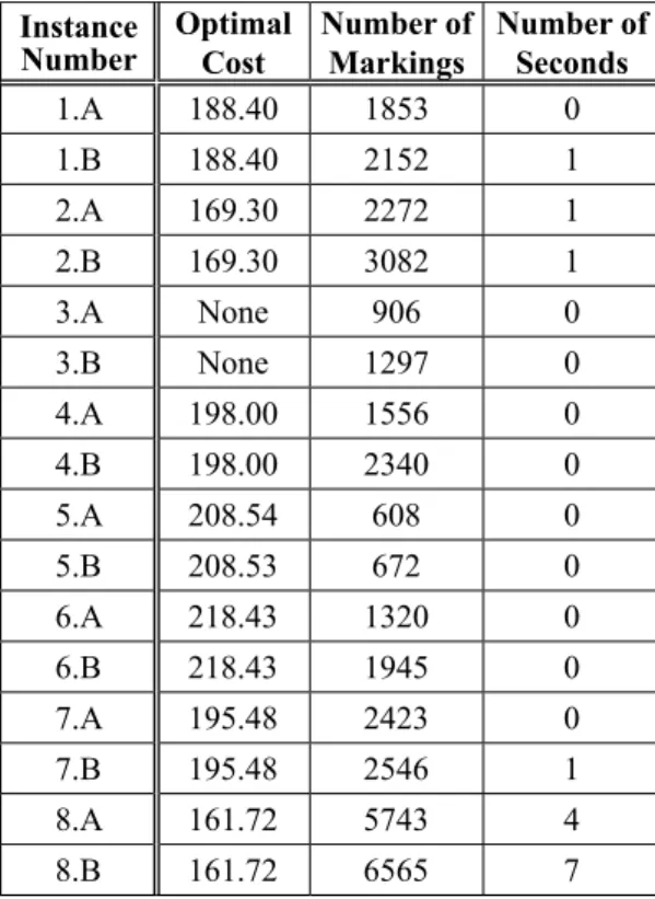
Lastly, we show the results of applying our ap-proach on several system instances. The system instances were obtained by random shuffling of the elements of the matrices T and K of the case study in Subsection 3.1. The details of the system instances can be obtained by contacting the author. Table 5 shows the optimal costs ob-tained using the CPN approach for eight system instances. For each instance, the table shows the optimal cost when including both constraints (case A) and when excluding Constraint II (case B). We verified the results by comparing them with the optimal costs obtained when us-ing exhaustive search. Note that for the instanc-es 3.A and 3.B, there is no feasible allocation. In such cases, the list of markings that are returned by the second application of SearchNodes (see Figure 4) is empty. For this part of the evalua-tion, we did not use the branching options.
5. Conclusion and Future Work
In this paper, we presented several improve-ments to the CPN-based approach for software component allocation on heterogeneous sys-tems. We incorporated the costs of communi-cation between the software components in the CPN model. Also, we explored the use of the
branching options in the CPN ML state space generation tool to scale the CPN approach to larger systems.
One potential limitation of the CPN-based ap-proach is the exponential increase in the gener-ated state space for larger systems. In this paper, we suggested a technique to determine an upper bound on the cost and only generate the states having cost less than this upper bound. The up-per bound can be determined using heuristics such as genetic algorithms. This significantly cuts down the generated state space.
However, the generated state space can become intractable for larger systems. Thus, it is of in-terest to explore the ways to generate and ana-lyze the state space more intelligently. For ex-ample, the work of [27] surveys several parallel algorithms to solve discrete optimization lems such as the component allocation prob-lem. A discrete optimization problem is often formulated as the problem of finding a path in a graph (the state space graph) from a designat-ed initial node to one of several possible final nodes. The authors review several techniques to search the state space and discuss how these
Table 2. Evaluation results including both constraints.
Optimal Cost − Exhaustive Search 153.43
Runtime in Seconds − Exhaustive Search 1.52
Optimal Allocation − CPN Approach (1, 3, 1, 3, 1, 1, 4, 3, 3, 2, 2)
Optimal Cost − CPN Approach 153.43
Number of Markings − CPN Approach − No Branching Options 16813
Number of Seconds − CPN Approach − No Branching Options 36
Number of Markings - CPN Approach − With Branching Options 2313
Number of Seconds - CPN Approach − With Branching Options 1
Table 3. Evaluation results excluding constraints II.
Optimal Cost − Exhaustive Search 144.50
Runtime in Seconds − Exhaustive Search 1.50
Optimal Allocation − CPN Approach (1, 2, 1, 1, 1, 4, 4, 2, 2, 3, 2)
Optimal Cost − CPN Approach 144.50
Number of Markings − CPN Approach − No Branching Options 27745
Number of Seconds − CPN Approach − No Branching Options 109
Number of Markings - CPN Approach − With Branching Options 3703
Number of Seconds - CPN Approach − With Branching Options 1
Table 4. Evaluation results excluding both constraints.
Optimal Cost − Exhaustive Search 144.50
Runtime in Seconds − Exhaustive Search 1.54
Optimal Allocation − CPN Approach (1, 2, 1, 1, 1, 4, 4, 2, 2, 2, 2)
Optimal Cost − CPN Approach 144.50
Number of Markings − CPN Approach − No Branching Options 103863
Number of Seconds − CPN Approach − No Branching Options 2193
Number of Markings - CPN Approach − With Branching Options 8741
Number of Seconds - CPN Approach − With Branching Options 6
Table 5. Evaluation results for different system instances.
Instance
Number Optimal Cost Number of Markings Number of Seconds
1.A 188.40 1853 0
1.B 188.40 2152 1
2.A 169.30 2272 1
2.B 169.30 3082 1
3.A None 906 0
3.B None 1297 0
4.A 198.00 1556 0
4.B 198.00 2340 0
5.A 208.54 608 0
5.B 208.53 672 0
6.A 218.43 1320 0
6.B 218.43 1945 0
7.A 195.48 2423 0
7.B 195.48 2546 1
8.A 161.72 5743 4