On the Sensitivity of Aggregative
Multiobjective Optimization Methods
Yann Collette
1and Patrick Siarry
21Technocentre Renault, Guyancourt, France 2Universit´e Paris 12, Cr´eteil, France
In this paper, we present a study on the sensitivity of ag-gregation methods with respect to the weights associated with objective functions of a multiobjective optimization problem. To do this study, we have developped some measurements such as the speed metric or the distribution metric. We have performed this study on a set of biobjec-tive optimization test problems: a convex, a non-convex, a continuous and a combinatorial test problems.
We show that some aggregation methods are more sensitive than others.
Keywords: multiobjective optimization, Chebyshev, weights, aggregation, metrics, performance, random, stochastic
1. Introduction
1.1. Introduction to Multiobjective Optimization
The multiobjective optimization has been a grow-ing domain of interest since approximately 1990 [4]. A lot of methods have been developed so as to solve a multiobjective optimization problem. Many of these methods use a genetic algorithm to solve this problem without transforming it into an “equivalent” monobjective optimization problem, but most of the methods use a transfor-mation to return to a monobjective optimization problem.
An example of the problem we are dealing with in multiobjective optimization is the following:
minimize f1(x)
minimize f2(x)
with x∈S⊂Rn
This example is a biobjective optimization prob-lem.
When we perform an optimization, we must keep in mind the definition of an optimum solu-tion. In monobjective optimization, this defini-tion is easy to understand. But, in multiobjec-tive optimization, we use a different form of def-inition for an optimum solution. And such a so-lution to a multiobjective optimization problem will be called a Pareto optimum solution. Let’s consider a multiobjective optimization problem withmobjective functions to be minimized. A solutionAis optimal with respect to a solution Bif:
x2 f2
f1 x1
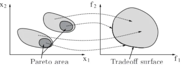
Figure 1.The tradeoff surface and the Pareto area.
• the objective function values of the so-lution A are as good or better than the objective function values of the solution B(∀i∈ {1,· · ·,m}fi(A)≤fi(B));
• the solutionAoutperforms the solutionB for at least one objective(∃i∈ {1,· · ·,m}
fi(A)<fi(B)).
Indeed, all these solutions belong to a hypersur-face and this locus of optimal solutions is called the tradeoff surface or the Pareto frontier (see Figure 1).
Not all these transformation methods(also called aggregation methods)are equivalent. Some of these transformations are sufficiently “efficient” so as to deal with a non convex multiobjective optimization problem and some of them aren’t [3]. But, when one has chosen a method, one has to overcome the problem of choosing some weight coefficients so as to underline the trade-off one is willing to do [1]. As we shall see, the problem of choosing a set of weights is not really critical because some methods are not re-ally sensitive to a weight variation and so, one can give “raw” weights to the method to model a tradeoff.
We present a study on the sensitivity of aggre-gation methods with respect to the weights as-sociated with objective functions of a multiob-jective optimization problem. To do this study, we have developed some measurements such as the speed metric or the distribution metric. We have performed this study on a set of biob-jective optimization test problems: a convex, a non-convex, a continuous and a combinatorial test problems. The results make us conclude that some aggregation methods are more sensi-tive than others.
In section 2, we present the various apparatus we used to perform our experiments: the opti-mization method, the aggregation methods, the metrics and the test problems. In section 2, we present the various steps followed during the experiment. In section 3, we present the
re-sults computed during the experiment and we conclude in section 4.
2. Description of the Experiment
Our aim is to study the influence of the aggre-gation method on the locus we reach on the Pareto surface, with respect to a certain amount of randomness in the optimization method.
We will try to quantify the amount of stochas-tic effect in the MOSA method [5]. We will also try to rank the main aggregation meth-ods (the weighted sum of objective functions, the Chebyshev method and the hybrid method) with respect to their sensibilities to a variation of weights.
In order to test the random level of an optimiza-tion method, we have built a new optimizaoptimiza-tion method: a local search method with a fixed probability of accepting a bad solution. This algorithm is described on algorithm 1.
By using this algorithm, we try to model the behavior of the simulated annealing with a con-stant temperature. With a real simulated anneal-ing, the probability of accepting a bad solution depends on the level of the objective function associated with the solution. So, when the tem-perature is constant, the probability of accepting a bad solution is likely to change.
Nevertheless, the randomized local search in the main line models the simulated annealing with a constant temperature.
Algorithm 1The randomized local search
paccept probability of accepting a bad solution
xcurr the current solution
Neigh(x) returns a neighbor solution of solutionx f() objective function to optimize
Niter number of iterations to perform
fori=1toNiter
x =Neigh(xcurr)
iff(x)≤f(xcurr)thenxcurr =x
iff(x)>f(xcurr)andrand(0,1)<paccept thenxcurr =x
2.1. The Aggregation Methods
2.1.1. The Weighted Sum of Objective Functions
The first method we used is a classical method in multiobjective optimization. We calculated the weighted sum of objective functions so as to aggregate objectives and have an equivalent single objective function to be optimized. This method(see in[4])is defined as follows:
feq(x) = Nobj
i=1
ωi·fi(x)
where:
• fiis the objective function number i of the
multiobjective optimization problem,
• Nobj is the number of objectives in the
multiobjective optimization problem,
• ωi is the weight associated with the
ob-jective function number i,
• xis the decision vector,
• feqis the single objective function.
This method shows poor performances on non-convex solution sets. It can’t find the solutions hidden in non-convexities of the Pareto frontier (see in[3]or in[1]).
2.1.2. The Chebyshev Aggregation of Objective Functions
Another way to aggregate objective functions is to use the Chebyshev distance (see in [4]). This way of aggregating objective functions is a very efficient one, it can find solutions hidden in non-convexities of the Pareto frontier. This distance is defined as follows:
feq(x) = max
i=1,···,Nobjωi·(
fi(x)−Fi)
For this method, theFi’s correspond to an ideal
bound for the objectivefi. Because sometimes
it’s hard to find good bounds for this method, we have decided to change the expression of the Chebyshev method:
feq(x) = max i=1,···,Nobj(
1−ωi)·(fi(x)−Fi)
whereFirefers to a limit on the objectivefi
un-der which the values offiare interesting for the
decision maker.
The notations are the same as those defined above.
2.1.3. The Hybrid Aggregation of Objectives Functions
Another way to aggregate objective functions is to use the Hybrid distance(see in[4]). This way of aggregating objective functions is nearly as efficient as with the Chebyshev one. It can find solutions hidden in non convexities of the Pareto frontier if theKparameter is well tuned. This distance is defined as follows:
feq(x) = max
i=1,···,Nobjωi·(fi(x)−Fi)
+K·
n
i=1
ωi·fi(x)
As with the Chebyshev method, we will use a transformed expression of the hybrid method which is related to the transformed expression of the Chebyshev method:
feq(x) = max i=1,···,Nobj(
1−ωi)·(fi(x)−Fi)
+K·
n
i=1
ωi·fi(x)
For this method, we performed some experi-ments so as to tune the value of the coefficient K. We used the non convex TRIGO test prob-lem. We searched the value ofK for which the distribution of solutions along the Pareto surface was as near as possible to the distribution of so-lutions we have obtained with the Chebyshev method and 100 equally distributed weights.
2.2. The Metrics Used
2.2.1. The Distribution Metric
first requirement implies knowing the analyti-cal expression of the tradeoff surface of the test problem. Having computed this set of solutions, one has to translate it using two vectorsv and
−v. Then, one builds cells around an area of the tradeoff surface by linking 4 neighbor solutions (see Figure 2).
2 1
0 0 1 2
Distribution metric
f1
f2
f1, f2 plane
Figure 2. The shape of the distribution metric.
This metric is easy to use: one has to put a threshold frontier so as to stop the optimization when all the solutions are lying inside the cells, then one counts the solutions in the cells and reports these results on a bar chart.
2.2.2. The Speed Metric
One way to compute the speed of an algorithm in single objective optimization is to set a thresh-old (over the global optimum value) and wait for the algorithm to reach this threshold. To be able to use this kind of “speed measurement”, we must use a test problem for which the lo-cal minima are well known. Using such a test problem, we will be able to size the value of the threshold correctly.
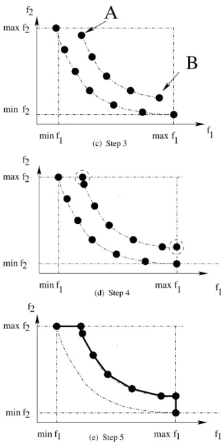
It is relatively easy to translate this idea for mul-tiobjective optimization, with the same limita-tions as with the single objective optimization test problem: we must work with a biobjective test problem. To compute the threshold frontier, we follow the steps illustrated in Figure 3. Step 1: compute the theoretical Pareto frontier (see Figure 3a)
Step 2: move the theoretical Pareto frontier us-ing a threshold vectorv (see Figure 3b). The amplitude of v is not really important, but it must be sufficiently important so as to catch a set of Pareto efficient solutions. The translation of the Pareto frontier using vector −v is per-formed so as to be sure to surround all the points in a cell defined by 2 Pareto efficient points( be-tween these 2 points, we can have some solu-tions which can be under the line joining these 2 points).
Step 3: remove points above arg maxf2and
be-low arg minf2
Step 4: add two points (f1(A),maxf2) and
(maxf1,f2(B)) (see Figure 3c)
Step 5: add two points (minf1,maxf2) and
(maxf1,minf2) (see Figure 3d)
Step 6: sort points in an increasing order, con-sidering the first objectivef1and the threshold
frontier are defined by the path linking all these points(see Figure 3e)
f2
f1 (a) Step 1
f1 f2
v
f1
f1 f1
f2 f2
f2
A
B
maxmin
max min
(c) Step 3
f1 f1
f2
f2
f2
f1 min
max min
max
(e) Step 5
Figure 3.How to build a treshold frontier in the speed metric.
Let us use the following notation:
• xTF
i theithpoint of the threshold frontier
• xS
j thejthpoint of the solution set
To perform the test, we follow these steps for eachxSi ∈S:
Step 1: find i such as f1xTFi
≤ f1(xSj) ≤
f1xTFi+1
Step 2: we denote f2(x) = A·f1(x) +B the
line between the points f1xTFi
,f2xTFi
and f1xTFi+1,f2xTFi+1: if
f2
xS
j
−A·f1
xS
j
−B≤0then the point
f1xSi
,f2xSi
is under the threshold frontier
To use the threshold frontier as a test to stop the running of a multiobjective optimization method, we can count the number of points that fall under the threshold frontier. If all the points(or a fraction like 90% for example)are under the threshold frontier, we stop the opti-mization method and check how many iterations were necessary to move all the points under the threshold. The theoretical Pareto frontier doesn’t need to verify any convexity hypothesis. The speed metric can be applied to any kind of multiobjective optimization problem since we are able to compute the theoretical Pareto fron-tier.
This stopping test for multiobjective optimiza-tion methods seems a good one to measure the speed of a method.
2.3. The Test Problems
2.3.1. The Continuous Test Problems
To be able to perform our experiments, we need a set of test problems so that we can easily move the starting point of the optimization and start closer to or farther from the Pareto set. Such a test problem doesn’t exist in the published set of multiobjective test problems. So we have de-veloped a simple set of test problems for which we can tune easily the position of the starting point with respect to the Pareto set. This set of test problems covers the classical difficulties we meet in multiobjective optimization: non-convexity, discontinuities, etc.
We will consider the following test problems:
The convex TRIGO1 test problem
minimize f1(θ,x) =1−cos(θ) +x
minimize f2(θ,x) =1−sin(θ) +x
The convex TRIGO2 test problem
minimize ⎧ ⎨ ⎩
f1(θ) =1−cos(θ) +x if 0≤x≤0.25
f1(θ) =1−cos(θ) +0.25·x+ 163 if 0.25≤x≤0.75
f1(θ) =1−cos(θ) +2.5·x−1.5 if 0.75≤x≤1
minimize ⎧ ⎨ ⎩
f2(θ) =1−sin(θ) +x if 0≤x≤0.25
f2(θ) =1−sin(θ) +0.25·x+ 163 if 0.25≤x≤0.75
f2(θ) =1−sin(θ) +2.5·x−1.5 if 0.75≤x≤1
with 0≤θ ≤ π2 and 0≤x≤1
The convex TRIGO3 test problem
minimize ⎧ ⎨ ⎩
f1(θ) =1−cos(1.5·θ) if 0≤θ ≤ π8
f1(θ) =1−cos(0.5·θ + π8) if π8 ≤θ ≤ 38·π
f1(θ) =1−cos(1.5·θ − π4) if 38·π ≤θ ≤1
minimize ⎧ ⎨ ⎩
f2(θ) =1−sin(1.5·θ) if 0≤θ ≤ π8
f2(θ) =1−sin(0.5·θ + π8) if π8 ≤θ ≤ 3·π8
f2(θ) =1−sin(1.5·θ − π4) if 38·π ≤θ ≤1
with 0≤θ ≤ π2 and 0≤x≤1
We find the analytical expression of the trade-off surface withx = 0. The expression of this surface is the following:
f1(θ) =1−cos(θ)
f2(θ) =1−sin(θ)
with 0≤θ ≤ π2
We have the same expression for the TRIGO3 test problem if we don’t consider the point den-sity variation with respect toθ.
We will also use a non convex form of the pre-ceding problem. The analytical expression of this problem is similar to the convex one. We just have to change 1−cos()and 1−sin()into cos()and sin()respectively.
2.3.2. The Combinatorial Test Problems
We will apply a continuous to combinatorial( bi-nary, to be more precise)transformation, so as to use the same kind of test problem in the con-tinuous space and in the combinatorial space. To obtain the combinatorial test problem:
• we define a binary size for the contiuous variablesxandθ (for example 8 bits);
• the variation interval of the binary vari-able is included between 0 and 2N−1;
• this variation interval is normalized to the variation interval[xmin,xmax]and[θmin,θmax].
So, we find the typical behavior of the combina-torial problems(huge variation of the objective function when we change the value of one bit on the combinatorial variable) while keeping the ability to visualize the behavior of the opti-mization method. For example, we can:
• visualize the movements of the current point in two dimensions during the opti-mization;
• choose accurately the position of the ini-tial point (we choose the initial value by using the continuous form of the test prob-lem, then we convert this value into a bi-nary one by following the steps we have described previously);
• build a parallel between the behavior of a combinatorial optimization method and a continuous optmization method by com-paring the trajectories of both methods.
2.4. The Experiment
For each problem, we proceed as follows: 1. We choose an initial point which allows us
2. We compute the weights so as to find solu-tions equally spaced along the tradeoff sur-face. To do so, we take the extreme points of the tradeoff surface ((1,0)and (0,1)), we draw a line between these two points, then we divide this line into as many pieces as we need couples of weights. We then com-pute the line which goes through the initial point and through one of the points of the preceding line, then we identify the lead-ing coefficient of the line with the desired couple of weights.
3. We place a threshold frontier close to the tradeoff surface. So, when the generated points are sufficiently close to the tradeoff surface, the optimization stops.
4. We apply the distribution metric which has the shape described in Figure 2.
The experiment follows these steps:
1. Choice of the initial point (π/4,1)and ini-tialization of the couple of weights to (0.5,0.5).
2. Initialization of the optimization method. 3. Initialization of the random number
genera-tor with a given random seed.
4. Execution of the optimization method, then returning to step 3. We reproduce this step 100 times.
5. We apply the distribution metric to the com-puted solutions to compute the distribution of solutions along the tradeoff surface. 6. x = x−Δx then returning to step 2. We
reproduce this step untilx=0.
We will execute two kinds of experiments using this test problem:
• An experiment with the continuous test problem.
• An experiment with the continuous test problem converted into a combinatorial one.
3. Results
3.1. The Graphs
We will present two kinds of graphs:
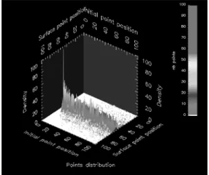
• graphs related to the distribution of points along the Pareto surface, with respect to
the probability of accepting a bad solu-tion and with respect to the posisolu-tion of the initial point.
• graphs related to the number of iterations required to reach the Pareto surface, with respect to the position of the initial point and to the probability of accepting a bad solution.
These graphs have special scales:
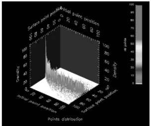
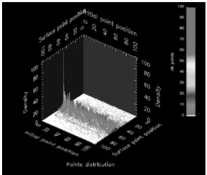
Graphs showing distribution of the points
• The dimension entitled “Initial point posi-tion” has a scale which spreads from 0 to 100 where 0 corresponds to the position of the initial point on the Pareto surface and 100 corresponds to the position of the initial point at a distance 1 from the Pareto surface.
• The dimension entitled “Surface point po-sition” has a scale which spreads from 0 to 100, where 0 corresponds to the po-sition θ = 0,x = 0 on the Pareto sur-face and 100 corresponds to the position θ =π/2,x=0 on the Pareto surface.
• The dimension entitled “Density” has a scale which spreads from 0 to 100 where 0 corresponds to no points counted at this position on the Pareto surface and 100 corresponds to all points counted at this position on the Pareto surface.
Speed graph
• The dimension entitled “Initial position” has a scale which spreads from 0 to 100. The meaning of these values is the same as in the “Initial point position” in the dis-tribution graph mentioned above.
• The dimension entitled “Probability” has a scale which spreads from 0 to 10 where 0 corresponds to the probability of accept-ing a bad solution of 1 and 10 corresponds to the probability of accepting a bad solu-tion of 0.
3.2. Some Results
The Chebyshev method and the continuous test problem
First, we tested the Chebyshev method on the convex and continuous test problems. The re-sults we have obtained with this test problem are represented in Figures 4a, 4b, 5a. The speed diagram is represented in Figure 5b.
Figure 4a.Probability 0.9.
Figure 4b.Probability 0.5.
Figure 4.Results for the continuous test problem: the Chebyshev method for probabilities 0.9 and 0.5.
The conclusions we can draw about this experi-ment are the following:
• When the probability of accepting a bad solution reaches 0, the distribution of points along the Pareto surface is concentrated on the locus designated by the direction given by the couple of weights. This is a
normal behavior of a multiobjective opti-mization method.
• When considering the speed diagram, the closer the initial point to the Pareto sur-face, the less iterations we need to reach the Pareto surface. The closer to 0 the probability of accepting a bad solution, the less iterations we need to reach the Pareto surface. Again, this is a normal behavior of a multiobjective optimization method.
Figure 5a.Probability 0.1.
Figure 5b.The speed diagram 0.5.
Figure 5.Results for the continuous test problem: the Chebyshev method for probability 0.1 and the speed
diagram. The Chebyshev method and the combinatorial test problem
Figure 6a.Probability 0.1.
Figure 6b.Probability 0.2.
Figure 6.Results for the combinatorial test problem with a 64 bits variable: the Chebyshev method for
probabilities 1.0 and 0.2.
The conclusions we can draw are rather inter-esting:
• We have nearly the same influence of the probability of accepting a bad solution on the distribution of points as with the con-tinuous case. The main difference lies in the fact that the distribution evolves rather abruptly with respect to the probability of accepting a bad solution. Between 1.0 and 0.3, 0.4, the distribution is still the same as in Figure 6a. Then, between 0.3, 0.4 and 0.0, the distribution evolves quickly to look like the distribution of the contin-uous case.
• For the speed diagram, it is completely different from the continuous case. The initial position has no influence on the
number of iterations needed to reach the Pareto surface. This is due to the combi-natorial aspect of the problem. A small change in the value of a bit can induce a huge change in the value of the objective function. The meaning of “being closer to the Pareto surface” seems to lose its meaning.
We can notice a change in the shape of the speed diagram when we are closer to the Pareto surface: an overcost in terms of iterations num-ber appears. This is certainly due to the neigh-borhood used: we have a mean change of 3 bits between a point and its neighbor. When we are really close to the Pareto surface, less than 3 bits need to be changed, so, to reach the Pareto surface, we first need to go back and then go forth. This movement induces an overcost in term of the number of iterations. This behavior has been observed in[2].
Figure 7a.Probability 0.1.
Figure 7b.The speed diagram.
Figure 7.Results for the combinatorial test problem with a 64 bits variable: the Chebyshev method for
The weighted sum of objective functions and the combinatorial test problem
We will now perform the same experiments on the same combinatorial test problem, but with the weighted sum of objective functions. The points distribution obtained are represented in Figures 8a, 8b and 9a. The speed diagram is represented in Figure 9b.
Figure 8a.Probability 1.0.
Figure 8b.Probability 0.2.
Figure 8.Results for the combinatorial test problem with a 64 bits variable: the weighted sum of objective
functions for probabilities 1.0 and 0.2.
The conclusions we can draw are the following:
• The points are distributed on a wider area than with the Chebyshev method. We still have the “brutal” change in the shape of the distribution of points with respect to the probability of accepting a bad solu-tion. Between a probability of 1 and 0.3,
Figure 9a.Probability 0.1.
Figure 9b.The speed diagram.
Figure 9.Results for the combinatorial test problem with a 64 bits variable: the weighted sum of objective
functions for probability 0.1 and the speed diagram.
0.4, the shape of the distribution of points is still “the same”. But between a proba-bility of 0.3, 0.4 and 0.0, the shape of the distribution of points changes quickly.
• We have a smaller overcost in terms of the number of iterations needed to reach the Pareto surface. This overcost doesn’t appear clearly in Figure 9b, but it appears in other figures not represented here.
• We can also notice that we need less it-erations to reach the Pareto surface than with the Chebyshev method. This differ-ence can be explained theoretically and is due to the way an aggregation method “follows” a direction given by a couple of weights.
objective functions and the Chebyshev method is that the Chebyshev method is efficient on multiobjective problems with a Pareto surface with a non convex shape, whereas the weighted sum of objective functions isn’t.
The hybrid method and the combinatorial test problem
Finally, we perform the same experiments on the hybrid aggregation method. The results are represented in Figures 10a, 10b and 11a. The speed diagram is represented in Figure 11b.
Figure 10a.Probability 0.1.
Figure 10b.Probability 0.2.
Figure 10.Results for the combinatorial test problem with a 64 bits variable: the hybrid method for
probabilities 1.0 and 0.2.
Figure 11a.Probability 0.1.
Figure 11b.The speed diagram.
Figure 11. Results for the combinatorial test problem with a 64 bits variable: the hybrid method for
probability 0.1 and the speed diagram.
The conclusions we can draw are the following:
• First, let us recall that the hybrid method is efficient on multiobjective problem with Pareto surfaces of a non convex shape(it depends on the value of the coefficientK).
• All the results are “between” the results we obtained with the Chebyshev method and the results we obtained with the wei-ghted sum of objective functions.
– The number of iterations required to reach the Pareto surface is more important than the number of iter-ations required to reach the Pareto surface using the weighted sum of objective functions, but it is less important than the number of iter-ations required to reach the Pareto surface with the Chebyshev method. The same kind of experiments were performed on various pairs of weights. The results were the same as with the pair(0.5,0.5).
4. Conclusions
These various experiments show a change in the shape of the distribution of points along the Pareto surface, with respect to the probability of accepting a bad solution.
We can observe two types of behavior:
• A behavior insensitive to the value of the probability of accepting a bad solution. In that case, the distribution of points is centered around the direction given by the couple of weights(0.5,0.5), but the distri-bution is really spread around this point. This induces that we can’t reach accu-rately this point on the Pareto surface.
• A behavior sensitive to the value of the probability of accepting a bad solution. In that case, for some values of probabil-ity, we can reach accurately a locus on the Pareto surface.
We can conclude that, when using the weighted sum of objective functions with a stochastic op-timization method, the choice of the weights is not really important because, due to the stochas-tic effect, we will not reach accurately a locus on the Pareto surface, but rather roughly. We also notice the changes which intervene on the speed diagram. When no perturbation on the distribution of points appears, the resulting speed diagram is independent of the probability of accepting a bad solution.
On the first speed diagram, we can notice the relative independence in terms of performances, with respect to the position of the initial point. This can be explained by the “complexity” of the
neighborhood we have used. When a large num-ber of bits are modified on the binary variable, at each iteration the distance we walk is very important. This implies that the initial point position is either close or far from the Pareto surface, after the first iteration the current point reaches more or less the same position.
We also observe an interesting phenomenon: the more the initial point is close to the Pareto surface, the more it appears an overcost in terms of iterations number. This can be explained by the complexity of the neighborhood we used. The more we have bits changing, the more im-portant is the distance walked in one iteration. So, when we are close to the Pareto surface(at a distance of 1 bit to change for example), we must first go back before being able to reach the optimal point on the Pareto surface.
Once a certain probability threshold is passed, the behavior of the distribution of points along the Pareto surface tends to come close to the be-havior we found with the continuous problem. Another phenomenon can be observed when considering the speed diagram and a neigh-borhood where 75% of the bits are changed (experiment not represented here). When the probability of accepting a bad solution is zero, we observe a very high overcost in terms of the number of iterations needed to reach the Pareto surface. There is a factor 10 between the part found using a probability of accepting a bad solution of 0.1 and the part found using a probability of accepting a bad solution of 0.0. This phenomenon is highlighted in the thesis of B. Krishnamachari[2]. We can imagine that for neighborhoods of high complexity, a min-imum probability of accepting a bad solution is needed to allow the optimization method to adapt its movements to avoid having to go back too often when the current solution is too close to the Pareto surface. This tells us that we must be really careful when choosing the initial so-lution of an optimization method: this soso-lution must be sufficiently close to the Pareto surface, but not too close.
References
[1] I. DAS, J. DENNIS, A Closer Look at Drawbacks of Minimizing Weighted Sums of Objectives for Pareto Set Generation in Multicriteria Optimization Problem.Structural Optimization,19,(1997), Issue 1, 63–69.
[2] B. KRISHNAMACHARI, X. XIE, B. SELMAN, S.
WICKER, Performance Analysis of Neighborhood
Search Algorithms. Preprint, Janvier, 2000.
http://citeseer.nj.nec.com/293033.html [3] A. MESSAC, G. J. SUNDARARAJ, R. V. TAPPETA, J.
E. RENAUD, Ability of Objective Functions to
Gen-erate Points on Nonconvex Pareto Frontiers.AIAA Journal,38,(2000), Issue 6, 1084–1091
[4] K. MIETTINEN,Nonlinear Multiobjective
Optimiza-tion. Kluwer Academic Publisher, 1999.
[5] E. L. ULUNGU, J. TEGHEM, P. H. FORTEMPS, D.
TUYTENTS, MOSSA Method: A Tool for Solving
Multiobjective Combinatorial Optimization Prob-lems.Journal of Multicriteria Decision Analysis,8
(4) (1999), 221–236.
Received:February, 2006
Revised:May, 2007
Accepted:May, 2007
Contact addresses:
Yann Collette Renault – 68240 1 Av. du Golf 78288 Guyancourt, France e-mail:[email protected]
Patrick Siarry LISSI Universit´e Paris 12 61 Av. du G´en´eral de Gaulle 94010 Cr´eteil, France e-mail:[email protected]
YANNCOLLETTEgraduated from Ecole Normale Sup´erieure de Cachan, prepared his PhD thesis on multiobjective optimization at Electricit´e de France. He received the PhD degree from the University Paris 12, in 2002. He is now a research engineer at Renault SA and is working on the optimization of various industrial problems, such as the tuning of diesel engines, structural optimization, etc.