Complex Modeling of Matrix Parallel Algorithms

Published online July 30, 2014 (http://www.sciencepublishinggroup.com/j/ajnc) doi: 10.11648/j.ajnc.s.2014030501.11

ISSN: 2326-893X (Print); ISSN: 2326-8964 (Online)

Complex modeling of matrix parallel algorithms

Peter Hanuliak

Dubnica Technical Institute, Sladkovicova 533/20, Dubnica nad Vahom, 018 41, Slovakia

Email address:

To cite this article:

Peter Hanuliak. Complex Modeling of Matrix Parallel Algorithms. American Journal of Networks and Communications. Special Issue: Parallel Computer and Parallel Algorithms. Vol. 3, No. 5-1, 2014, pp. 1-14. doi: 10.11648/j.ajnc.s.2014030501.11

Abstract:

computers and algorithms too). In this sense the paper is devoted to a complex performance evaluation of matrix parallel algorithms (MPA). At first the paper describes the typical matrix parallel algorithms and then it summarizes common properties of them to complex performance modeling of MPA. To complex performance analysis we are able to take into account all overheads influence performance of parallel algorithms (parallel computer architecture, parallel computation, communication etc.). To be le to analyze MPA in their abstract form we have defined needed decomposition models of MPA. For these decomposition strategies we derived analytical relation for defined complex performance criterions including isoefficiency functions, which allow us to predict performance although for hypothetical parallel computer. In its experimental part the paper considers the achieved results using defined complex performance criterions including issoefficiency function for performance prediction also for hypothetical future parallel computers. Such idea of common abstract analysis could be very useful in deriving complex performance criterions for groups of other similar parallel algorithms (PA) as for example numerical integration PA, optimization PA etc.

Keywords:

Performance Modeling, Optimization, Overhead Function H (S, P), Inter Process Communication IPC, Performance Prediction, Issoeficiency Function

1. Trends in Parallel Computing

Basic common properties in parallel computing (parallel computers, parallel algorithms) computing, which are reaching continuous demands to performance acceleration, are as follows

embedded parallel principles on various levels of technical (hardware) and program support means (software) [8]

using of homogenous shared resources so in computing nodes of parallel computers (processors, cores, computers) as in parallel algorithms too [24] using of high speed communication networks reducing communication latency [39]

increased client/server computing on symmetrical multiple processors or cores (SMP)

trends to unified modeling of parallel computers (shared memory, distributed memory) and in parallel algorithms (shared memory, distributed memory, hybrid)

continuous demands to increase mobility and data

migration [23]

the development of hardware neutral parallel programming language, such as Java, provides a virtual computational environment in which computing nodes of parallel computer appear to be homogenous

continuous improvements in network technology and communication middleware in order to use shared parallel resources in unified manner (cloud computing, Internet computing).

systems [38]. A member of NOW module or Grid could be any classic supercomputers [35].

2. Performance Evaluation in Parallel

Computing

To performance evaluation of parallel computers and parallel algorithms we can use evaluation methods as follows

analytical

application of queuing theory results [11, 21] order (asymptotic) analyze [12, 20]

Petri nets [7] simulation methods [25] experimental

benchmarks [28] modeling tools [32] direct measuring [9, 30].

Analytical method is a very well developed set of techniques which can provide exact solutions very quickly, but only for a very restricted class of models. For more general models it is often possible to obtain approximate results significantly more quickly than when using simulation, although the accuracy of these results may be difficult to determine.

Simulation is the most general and versatile means of modeling systems for performance estimation. It has many uses, but its results are usually only approximations to the exact answer and the price of increased accuracy is much longer execution times. They are still only applicable to a restricted class of models (though not as restricted as analytic approaches.) Many approaches increase rapidly their memory and time requirements as the size of the model increases.

Evaluating system performance via experimental measurements is a very useful alternative for computer systems. Measurements can be gathered on existing systems by means of benchmark applications that aim at stressing specific aspects of computers systems. Even though benchmarks can be used in all types of performance studies, their main field of application is competitive procurement and performance assessment of existing systems and algorithms.

3. Parallel Algorithms

In principal we can divide parallel algorithms (PA) to the following groups

parallel algorithm using shared memory (PAsm).

These algorithms are developed for parallel computers with shared memory as actual modern symmetrical multiprocessors (SMP) or multicore systems on motherboard

parallel algorithm using distributed memory (PAdm).

These algorithms are developed for parallel computers with distributed memory as actual NOW system and their higher integration forms named as

Grid systems

hybrid PA which combine using of both previous

PA (PAhyb). This trend support applied using of

NOW consisted from computing nodes based on SMP parallel computers.

The main difference between PAsm and PAdm is in form

of inter process communication (IPC) among created parallel processes [18, 33]. Generally we can say that IPC communication in parallel system with shared memory can use more communication possibilities (all the possibilities of communication in shared memory) than in distributed systems (only network communication).

2.1. Developing Steps of PA

The role of programmer is for the given parallel computer and for given application problem to develop the effective parallel algorithm. This task is more complicated in those cases, in which we have to create the conditions for any parallel activities in form of dividing the sequential algorithm to their mutual independent parts named parallel processes. Principally development of any parallel algorithms (shared memory, distributed memory, hybrid) includes performing of the following activities [29, 34].

decomposition of a complex problem to a set of

parallel processes including their data

(decomposition model)

mapping – distribution of decomposed parallel processes to computing nodes of used parallel computer

inter process communication (IPC) to cooperation (data communications, synchronization, control) of performed parallel processes

performance optimization (tuning) of developed parallel algorithm (effective PA).

The most important step is to choose for given complex problem optimal decomposition model. To do this there is necessary to understand given complex problem, shared data, applied sequential algorithms (SA) and the flow of SA control [4, 26].

3.1.1. Decomposition Models

3.1.2. Mapping

This step allocates created parallel processes to computing nodes of parallel computer for their parallel executions. There is necessary to achieve that every computing node should perform allocated parallel processes (one or more) with at least approximate input loads (load balancing) on real assumption of equal powerful computing nodes. Fulfillment of this condition contributes to optimal parallel execution time.

3.1.3. Inter process Communication

Inter process communication (IPC) represents a needed tool to cooperation of decomposed parallel processes. In general we can say that dominated parts of parallel algorithms are decomposed parallel processes (independent sequential parts) and inter process communication (IPC) among created parallel processes in performing of PA. We have been analyzed IPC communication in detail in [18].

3.1.4. Performance Optimization

After verifying developed parallel algorithm on used parallel computer the further step is performance modeling and its optimization in order to develop effective PA. This step contents analysis of previous steps in such a way to minimize whole execution time latency of parallel computing T(s, p). Performed optimization of T(s, p) for given parallel algorithm depends mainly from following factors

allocation of balanced input load to used computing nodes of parallel computer (load balancing) [1, 36] minimization of accompanying overheads amounts (parallelization, IPC, synchronization control of PA) [14, 22].

To do load balancing we need in case of obvious using of equally powerful computing nodes of PC results of load

allocation for given developed PA. In dominated parallel computers (NOW, Grid) there are necessary to reduce (optimize) mainly number of inter process communications IPC (communication complexity) for example by considering of alternative existing decomposition model.

3.2. Complex Performance Evaluation Metrics

To evaluating parallel algorithms we have been defined in [14] complex performance criterions of PA. Tradeoffs among these performance factors are often encountered in real applied PA. We summarize these criterions as follows

complex parallel execution time T(s, p) including overhead function h(s, p)

complex speed up S(s, p) complex efficiency E(s, p) issoeficiency w(s).

4. Typical Matrix Parallel Algorithms

Some of the typical matrix parallel algorithms we have been yet analyzed as follows

parallel matrix multiplication [16]

parallel fast discrete Fourier Transform (DFFT) in [14].

We will short describe further typical MPA.

4.1. System of Linear Equations

System of n linear equations (SLE) with n variables x1,

x2, x3, ..., xn, in matrix form is defined as follows [3, 10]

A . X = B

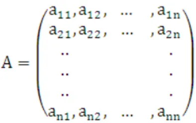
where the matrix A is a square matrix of coefficients, B is the vector of the right side and X is a vector of searching unknown as follows

A =

a , a , a , … a a , a , a , … a … … … a , a , a , … a

B = a ,

a ,

. . . . a ,

X = X

X . . . . X

4.1.1. Methods of SLE Solving

There is no known universal optimal method of solving systems of linear equations. There are several different ways of solving SLR whereby each of them at fulfillment of defined assumption implies the option of the solution method. In principle, we divide the available methods for exact (finite) and iterative. There exist many various ways how to solve system of linear equations. But there does not exist any optimal way of solving it. The existed methods can be divided into

exact

Cramer rule

Gaussian elimination methods (GEM) GEM alternatives

iterative

4.1.2. Typical Decomposition Models

To parallel solution of SLE by preferred Gauss eliminated method (GEM) the decomposition models are as follows [16]

allocation of block strips

• gradually allocation of strips.

Figure 1. Allocation of matrix data blocks.

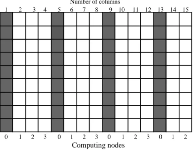
Another alternative decomposition model with gradual allocation of columns they are allocated columns to individual computing nodes like the card are gradually passing out at games to game participants. Illustration of gradual assignment of columns is at Fig. 2.

Figure 2. Allocation of matrix columns.

4.2. Partial Differential Equations

Partial differential equations (PDE) are the equation involving partial derivates of an unknown function with respect to more than one independent variable. PDEs are of fundamental importance in modeling all types of continuous phenomena in nature. Typical examples are weather forecasting, optimization of aerodynamic shapes, fluid flow, and the like. Simple PDE can be solved directly, but in general it is necessary to approximate the solution on the extensive network of final points by iterative numerical methods [18]. We will confine our attention to PDE with two space independent variables x, y. The needed function we denote as u (x, y). The considered partial derivations we denote as uxx, uxy, uyy etc. For practical use the most

important PDE are two ordered equations as follows heat equation, ut = uxx

wave equation, utt = uxx

Laplace equation uxx + uyy = 0.

These three types are the basic types of general linear second order PDR as in follows

uxx + b uxy +c uyy + d ux + e uy + f u + g = 0. This equation

could be transformed by changing the variables to one of three basic equations, including the members of the lower rows, provided that the coefficients a, b, c are not all equal to zero. Variable b2 – 4 ac is refer to as discriminant whereby its value determines the following basic groups PDR of second order

b2 – 4 ac > 0, hyperbolic (typical equation for waves).

b2 – 4 ac = 0, parabolic (typical of heat transfer) b2 – 4 ac < 0, elliptical (typical is the Laplace equation) [6, 37].

Classification of more general types of PDE is not so clear. When the coefficients are variable, then the type of equation can be modified by changes in the analyzed area and if it is intended at the same time with several equations, each equation can generally be of a different type. Simultaneously analyzed problem may be nonlinear or equation requires more than second order [2, 23]. Nevertheless, the basic used classification of PDE is also used when determining if it is not accurate. Specifically the following types of PDEs are as follows

hyperbolic. This group is characterized by time dependent processes that are not stabilized at some steady state

parabolic. Group characterized by a time dependent processes, which tend to the stabilization

elliptical. Group describes the processes that have reached steady state and are therefore time independent. A typical example is the Laplace equation.

Here we show how to solve in parallel way specific PDE – Laplace equation in two dimensions – by means of a grid computation method that employs finite difference method. Although we focus on this specific problem, the same techniques are used for solving other PDE (Laplace - three

dimensional, Poisson equation etc.), extensive

approximations calculations on various parallel computers (supercomputers, massive, SMP, NOW, Grid) eventually solving another similar complex problems.

4.2.1. Parallel Application of Iterative Algorithms

Here we show how to solve in parallel way specific PDE – Laplace equation in two dimensions – by means of a grid computation method that employs finite difference method. Although we focus on this specific problem, the same techniques are used for solving other PDE (Laplace - three

dimensional, Poisson equation etc.), extensive

approximations calculations on various parallel computers (supercomputers, massive, SMP, NOW, Grid) eventually solving another similar complex problems. Laplace equation is a practical example of using iterative methods to its solution. The equation for two dimensions is following

Number of columns

1 2 3 4 5 6 7 8 9 10 11 12 13 14 15

0 1 2 3 0 1 2 3 0 1 2 3 0 1 2

Computing nodes

Number of columns

1 2 3 4 5 6 7 8 9 10 11 12 13 14 15

0 1 2 3 0 1 2 3 0 1 2 3 0 1 2

2 2 0

2 2

x y

δ δ

δ δ

Φ₊ Φ₌

Figure 3. Grid approximation of Laplace equation.

Function Ф(x, y) could represent some unknown

potential, such as heat, stress etc. Given a two-dimensional region and values for points of the region boundaries, the

goal is to approximate the steady-state solution Ф(x, y) for

points in the interior by the function u(x, y). We can do this by covering the region with a grid of points (Fig. 1) and to obtain the values of u(xi, yj) = ui,j.

Let us consider square region (a, b) x (a, b). For coordinates of grid points is valid xi = i*h, yj = j*h, h = (b-a)

/ N for i,j = 0, 1, ..., N. We replace partial derivations of Ф

~ u(x, y) by the differences of ui,j. After substituting we

obtain final iteration formulae as

X_i,j(t+1) _{= (X}

i-1,j(t) + Xi+1,j(t) + Xi,j-1(t) + Xi,j+1(t) ) / 4

orits alternative version

X_i,j(t+1) _{= (4 X}

i,j(t) + Xi-1,j(t) + Xi+1,j(t) + Xi,j-1(t) + Xi,j+1(t) ) / 8

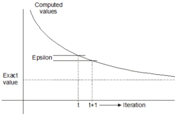
Each interior point is initialized to some value. The steady-state values of the interior points are then computed by repeated iterations. In each iteration the new point value is set to a combination of the previous values of neighboring points. The computation terminates either after a given number of iterations or when every new value is within some acceptable difference Epsilon > 0 of the previous value.

Figure 4. Convergence rate.

Illustration of convergence rate of iterative parallel algorithms is at Fig. 4. For the convergence of Gauss-Seidel iterative method is valid the same conditions as for Jacobi

iterative method whereby the Gauss-Seidel method converges faster. Given condition is not only necessary but only a sufficient one for the convergence of both methods. In practice, we use both iterative methods also in case of not satisfying of this condition based on them that convergence is influenced also by selection of initial vector.

4.2.1.1. Communication Model

For Jacobi finite difference method a two-dimensional grid is repeatedly updated by replacing the value at each point with some function of the values at a small fixed number of neighboring points. The common approximation structure uses a four-point stencil to update each element Xi,j (Fig. 5.).

Figure 5. Communication model for 4 - points approximation

Similar for more accurate value of any point we can also used more precise multipoint approximation relation, and that for example through approximation of nine points according the pencil at Fig. 6 with following relation

Xi,j(t+1) = (16 Xi-1,j(t) + 16 Xi+1,j(t) + 16 Xi,j-1(t) + 16 Xi,j+1(t)

- Xi-2,j(t) - Xi+2,j(t) - Xi,j-2(t) - Xi,j+2(t)) / 60

Figure 6. Stencil with nine points.

5. Complex analytical performance

modeling of MPA

Figure 7. Square matrix n x n.

The reason for preferred square matrix reducing of parameter number (n = m) in derivation process of complex analytical performance relations (execution time, speed up, efficiency, isoefficiency etc.). Such more transparent approach is supported with following additional reasons

any rectangular matrix n x m could be transformed into a square matrix n x n either by extending the number of rows (where m < n) or column (if m > n) derivation process of performance relations will be the same except for the fact that when considering the complexity of the matrix instead of n2 (square matrix) we have to consider product n. m .

5.1. Basic Common Characteristics of MPA

Typical characteristics of matrix parallel algorithms are regularities both in the program (matrix computational activities) and also in data structure matrix (matrix elements). Such regularity we refer to as a domain. Matrix computational activities we will represent as T(s, p)comp

latency. Considering square matrix n x n sequential

computational complexity is given as n2. Common

characteristics of matrix parallel algorithms (MPA) are as follows

parallelization - matrix itself is well parallelized theoretically up to level of its single data element. But applying such a maximal degree of parallelization could not be effective because of low computation complexity for one matrix element.

Therefore we will consider basic matrix

decomposition models in group of matrix data elements

using of domain decomposition models in which domain is represented by data matrix elements (data domain)

applied matrix date domain decomposition models define that for parallel computation on decomposed parts of matrix data elements there is necessary to perform in a parallel way the whole computation as in sequential matrix algorithms

to do any computational operation on matrix there is necessary to do this operation on every matrix element or group of them. From performed analysis comes out that at solving typical MPA parallel matrix computations are performed as follow

allocated matrix data part of given computing node are repeatedly evaluated according used

PA (iteration PA). After every iterations step

there is necessary to perform IPC

communication to neighboring computing nodes of shared matrix data elements

allocated matrix data part of given computing node in one computing step are reduced according used PA to simpler matrix data part (for example GEM PA). After every reduction step there is necessary to perform IPC communication to all other used computing nodes.

Based on these conclusions to modeling of MPA there is

necessary to derive needed computational and

communication complexity.

5.1.1. Computational Matrix Complexity

5.1.1.1. Sequential

Sequential computational matrix complexity for

considered square matrix n x n is given as n2 (computation

on each matrix element). Then the used asymptotic complexity is given as O(n2).

5.1.1.2. Parallel

Computational parallel matrix complexity Z(s, k) is given as computational complexity of one decomposed parallel process in k computing steps where parameter s we have been defined [14] as working load of given problem. For square matrix s = n2 (sequential matrix complexity). Through matrix decomposition models we are creating p parallel processes (matrix decomposition to p matrix parts) the Z(s, k) will be given as a quotient of computational

sequential matrix complexity n2 and number of

decomposed parallel processes p as follows

2 ( , ) ( ,1) n

Z s k Z s

p =

where Z(s, 1) represent computational complexity in one computation step. From derived relation the parallel computation time complexity T(s, p)comp is given through

quotient of parallel computing time running time of one

parallel process (product of its complexity Z(s, 1)comp and a

constant tc1 as an average value of performed computation

operations) through number of decomposed parallel processes p as follows

1 2_.

. ) 1 , ( )

p , (

p t n s

Z s

T comp = comp c

In MPA we are oft using mapping under the condition n

= p. Then we get for T(s, p)comp following simpler relation

as

1

. . ) 1 , ( )

p ,

(s _comp Z s _comp n t_c

T =

number of computation nodes p mathematical limit of T(s, p)comp is given as

0 . . ) 1 , ( lim )

p ,

( 1

2 =

= →∞

p t n s

Z s

T _{comp p} comp c

From this result we can see that a MPA the dominant influence will have mainly communication complexity. Therefore we will exanimate basic matrix decomposition models and their consequences to defined complex performance criterion.

5.2. Basic Matrix Decomposition Models

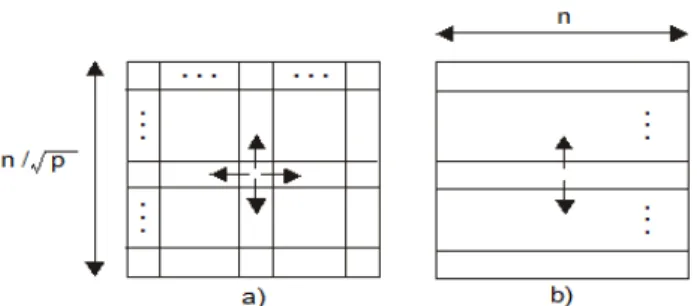
Supposed efficiency of parallel matrix algorithms (shared memory, distributed memory, hybrid) required to allocate a parallel process to more than one internal element of the square matrix (data elements). Then for decomposition of matrix elements to some groups of matrix data elements we have in principal two basic decomposition models as follows

decomposition model of n x n matrix to square blocks of matrix elements (parallel process). Illustration example of matrix decomposition to p blocks (B1, B2, …, Bp) is at Fig. 8 a. In this case the

decomposed blocks consist from at least four matrix data elements.

decomposition model of n x n to continual matrix strips of matrix elements. Continual strips consist of at least one matrix row or one matrix column. Illustration example of matrix decomposition to p strips (S1, S2, …, Sp) is at Fig. 8 b. In this case the

decomposed strips consist from at least one matrix row.

Figure 8. Matrix decomposition models a) blocks b) strips.

5.2.1. Decomposition Model to Blocks

For mapping matrix elements in blocks a inter process communication is performed on the four neighboring edges of blocks, which it is necessary in computation flow to exchange. Every parallel process therefore sends four messages and in the same way they receive four messages at the end of every calculation step (Fig. 9. a) supposing that all needed data at every edge are sent as a part of any message).

Figure 9. Communication decomposition models a) blocks b) strips.

Then the requested communication time for this decomposition model is given as

) (

8 )

,

( _{commb s} t_w

p n t p

s

T = +

using defined technical communication parameters [18] as follows

ts is defined parameter for communication

initialization

tw is defined parameter for data unit latency.

This equation is correct for p ≥ 9, because only under this assumption it is possible to build at least one square because only then is possible to build one square block with for communication edges. Using these variables for the communication overheads in decomposition method to blocks is correct

) (

8 ) , ( )

, ( ) p ,

( _{comm commb s} t_w

p n t p s h p

s T s

T = = = +

Then the requested communication time for this decomposition method is given as

) (

8 _{s w}

comb t

p n t

T = +

5.2.2. Matrix Decomposition to Strips

Decomposition method to rows or columns (strips) are algorithmic the same and for their practical using is critical the way how are the matrix elements putting down to matrix. For example in C language are array elements put down from right to left and from bottom to top (step by step building of matrix rows).

In this way it is possible send very simple through specification of the beginning address for a given row and through a number of elements in row (addressing with indexes). Let for every parallel process (strips) two messages are send to neighboring processors and in the same way two messages are received from neighboring processors (Fig. 8 b) supposing that it is possible to transmit for example one row to one message. Communication time for a calculation step T(s, p)comms is

then given as

(

)

4 )

,

(s p comms ts n tw

Using these variables for the communication overheads in decomposition method to strips is correct

) t (t 4 ) , ( ) , ( ) p ,

(s T s p h s p _s n _w

T _comm = _comms = = +

The whole time to execute parallel algorithm T(s, p) for decomposition to strips is then given in general as

w s 2 ) t (t 4 . ) p , ( n p t n s

T = c + +

In this case a communication time for one calculation step does not depend on the number of used calculation processors.

5.3. Complex Analytical Performance Modeling

To complex MPA performance modeling we have been defined as deriving of evaluation criterions of IPA including considering overhead function h(s, p). We summarized derived analytical results as following

Shared results for both decomposition models (blocks, strips)

execution time of sequential square matrix algorithm T(s, 1)

1 2 )

1 ,

(s _comp n t_c

T =

execution time for own parallel computation time of

IPA parallel algorithms T(s, p)comp

1 2 . ) , ( p t n p s

T _calc = c

optimal conditions to selection of matrix

decomposition model for ts ,and for tw respectively

w

s t

p n

t > (1− 2 ) w (1 2 ) ts.

p n

t > −

Different results for basic matrix decomposition models (blocks, strips)

overhead function for blocks h(s, p)b and for

strips h(s, p)s as follows

) (

8 ) ,

( b s tw

p n t p s

h = +

) t (t 4 ) ,

(s p _s n _w

h _s = +

complex parallel execution time for blocks T(s, p)compb, and for strips T(s, p)comps

1 2 ) ( 8 . ) , ( ) , ( ) p ,

( s w

c ipcb calc calcb t p n t p t n p s T p s T s

T = + = + +

1 2 ) ( 4 . ) , ( ) , ( ) p ,

( s w

c ipcs calc

calcs t nt

p t n p s T p s T s

T = + = + +

parallel speed up for blocks S(s, p)b, and for

strips S(s, p)s

) t t (p 8 ) , ( ) 1 , ( ) , ( w s 1 2 1 2 n p t n t p n p s T s T p s S c c calcb b + + = =

efficiency for blocks E(s, p)b, and for strips E(s,

p)s ) t t (p 8 ) , ( ) , ( w s 1 2 1 2 n p t n t n p p s S p s E c c b b + + = = ) ( 4 ) , ( ) , ( 1 2 1 2 w s c c s s t n t p t n t n p p s S p s E + + = =

constant C (needed constant in deriving an isoefficiency function w (s)) and that for blocks as Cb, and for strips as Cs in issoeficiency

function ) t t (p 8 ) , ( 1 ) , ( w s 1 2 n p t n p s E p s E

Cb c

+ = − = ) ( p 4 ) , ( 1 ) ,

( 2 ₁

w s c s t n t t n p s E p s E C + = − =

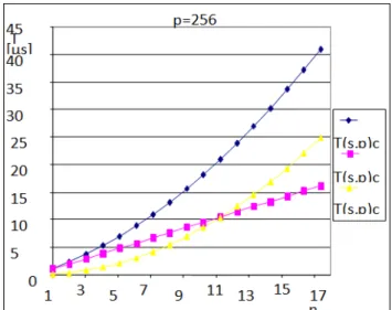
Fig. 10 illustrates growth dependencies of parallel

computing time T(s, p)comp, communication time T(s, p)comm

and complex parallel execution time T(s, p)complex from

input load growth n (Square matrix dimension) at constant number of computing node p = 256

Figure 10. Dependencies of T(s, p)complex,T(s, p)comm and T(s, p)comp from n ( p=256).

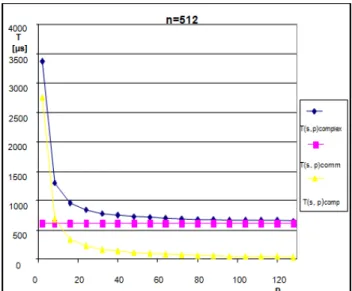
Fig. 11 illustrates growth dependencies of parallel

computing time T(s, p)comp, communication time T(s, p)comm.

and complex parallel execution time T(s, p)complex from

Figure 11. Dependencies of T(s, p)complex, T(s, p)comm and T(s, p)comp from p (n=512).

5.3.1. Issoeficiency Functions

Issoeficiency function w(s) is very important for performance prediction of parallel algorithms PA. For modeling of performance prediction in PA we are going to derive for defined basic matrix decomposition models (blocks, strips) corresponding analytical issoeficiency

functions w(s)b (Decomposition to blocks) and w(s)s

(decomposition to strips). For asymptotic complexity of w(s) is valid following derived relation as

[

]

max )

(s T s p calc

w =

where defined workload s is a function of input load n.

For IPA it is given as s = n2. We have defined that for given

value efficiency E(s, p) following quotient of efficiencies E(s, p) is constant

C E E ₌ −

1

5.3.1.1. Canonical Matrix Decomposition Models

As basic matrix decomposition models we have defined such matrix decomposition models to which there is possible to reduce all other known matrix decomposition models. Then the canonical matrix decomposition models are as follows

matrix decomposition model to blocks matrix decomposition model to strips.

For defined constants Cb (blocks) and Cs (strips) which

are integral parts of issoeficiency functions w(s)b (blocks)

and w(s) (strips) we have derived following relations

) t t (p 8 ) , ( 1 ) , ( w s 1 2 n p t n p s E p s E

Cb c

+ = − = ) ( p 4 ) , ( 1 ) , ( 1 2 w s c s t n t t n p s E p s E C + = − =

To win a closed form of issoeficiency function w(s)b,

w(s)s we have used an approach in which we performed at

first the analysis of increasing input load influenced the

analyzed expression contained ts in relation to p so to keep

this growth constant (we supposed that tw = 0). Then for

constants Cb, Cs we get following expressions

s c b t p t n C 8 1 2 = s c s t t n C p 4 1 2 =

From these expressions we can derive for searched functions w(s)b = w(s)s = n2 from relations for Cb, Cs

following relations 1 2 ₈ ) ( c s b b t t p C n s

w = =

1

2 4 p

) ( c s s s t t C n s

w = =

With a similar approach we can analyze the influence growth of input load caused another part of expression

from ts in relation to p so to keep this growth constant (we

supposed that ts = 0). Then after setting and performed

needed adjustments we get for searched functions w(s)b and

w(s)s following relations

1 2 8 ) ( c w b b t t n p C n s

w = =

1 4 ) ( c w s s t t p n C s w =

Final derived analytical functions w(s)band w(s)s are as

follows         = 1 1 1 2 8 , 8 , max ) ( c w b c s b c b t t p n C t t p C p t n s w         = 1 1 1 2 4 , 4 , max ) ( c w s c s s c s t t p n C t t p C p t n s w

5.3.1.2. Optimization of Issoefficiency Functions

Optimization of derived issoefficiency functions require to search for dominant expressions in derived final relations for w(s)b a w(s)s. For this purpose we have been done

comparison of individual expressions of w(s)b and w(s)s

with following conclusions

the first expressions of w(s)b and w(s)s are the same

and therefore this expression will be the component of final optimized w(s)opt. At the same time for this

expression at performed asymptotical analysis in relation to parameter p the following limit is valid

0 .

lim 1

2

=

→∞n _ptc

p

and therefore the similar first expressions of issoeficiency functions w(s)b and w(s)s we can omit

from searched w(s)opt

in relation to the similarity of actually first

expressions of w(s)b and w(s)s (After omitting

follows 1 1 4 8 c s s c s b t t p C t t p C ≥

This condition after reducing of shared expression parts lead to inequality 2 Cb≥ Cs. After setting and

following adjustments we get final condition as p ≥

1, which is valid on the whole range of spotted values of parameter p. It means the with this performed expression comparison we have got more dominated expression which we let to the next three

comparisons (Two from w(s)b and one from w(s)s)

in an analogous way we do comparison of third

expressions from original w(s)b and w(s)s

issoeficiency functions and that as follows

1 1 8 4 c w b c w s t t p n C t t p n C ≥

These conditions after reducing of shared expression parts lead to following inequality Cs√p ≥ 2 Cb. After

setting and performed adjustments we get final condition p ≥ 1, which is fulfilled on the whole range of parameter p. With performed comparison we have ignored further less expression and final relation w(s)opt is actually as follows

      = 1 1 8 , 4 max ) ( c s b c w s opt t t p C t t p n C s w

final comparison of remaining expression comes to following expression comparison

1 1 8 4 c s b c w s t t p C t t p n C ≥

This condition after reducing of shared expression parts leads to following inequality Cs n tw≥ 2 Cbts.

After setting and performed adjustments we come to following inequality n2. tw2≥√p ts2. This inequality

we are able to solve only for concrete values of parameters n, p, ts, tw. For example using following

values of parameters ts = 35 µs, tw = 0,23 µs and

under assumption of in praxis frequent case of choosing n = p we get simpler expression to condition validity as n. √n ≥ 152,172or p. √p ≥

152,172. The smallest integer number which satisfies

given condition is p = n = 813. Satisfying this condition for n or p, the final issoefficiency function

w(s)opt given with first expression and in opposite is

given with second expression of following final

optimized issoeficiency function w(s)opt

. 8 , 4 max ) ( 1 1       = c s b c w s opt t t p C t t p n C s w

5.3.1.3. Conclusions of Issoeficiency Functions

Then for the given concrete value of E(s, p) and for given values of parameters p, n we can in analytical way the thresholds, for which growth of isoefficiency function means decreasing of efficiency of given parallel algorithm with assumed typical decomposition strategies. This means the minor scalability of the assumed algorithm. In case of decomposition strategy the approach is similar to analyzed practical used decomposition matrix strategies.

Based on analysis of computer technical parameters ts, tw,

tc for some parallel computers in the world they are valid

following inequalities ts>>tw>tc. Alike is valid that p ≤ n.

Using these inequalities it is necessary to analyze dominancy influence of the all derived expressions.

Then the asymptotic issoefficiency function is limited through dominancy conditions of second and third expressions. From their comparison comes out

based on real condition tw≥ ts a third expression is

bigger or equal than a second expression and an issoefficiency function is limited through the first

expression of w(s)opt. If we used following technical

parameters ts = 35 µs, tw= 0,23 µs this is true for n

≥ 813

for n < 813 and for the same technical constants ts =

35 µs, tw= 0,23 µs issoefficiency function is limited

through a second expression of w(s)opt.

6. Results

We illustrate some of chosen performed tested results. To practical illustrations we have used MPA algorithms for iterative solving of Laplace PDE equation defined as follows

four point iteration relation in which in one iteration are performed five arithmertic operations (tc1 = 5 tc)

communication model according Fig. 5.

For experimental testing we have used workstations of NOW parallel computer (workstations WS 1 – WS 5) and supercomputer as follows

WS 1 – Pentium IV (f = 2,26 G Hz)

WS 2 - Pentium IV Xeon (2 proc., f = 2,2 G Hz) WS 3 - Intel Core 2 Duo T 7400 (2 cores, f=2,16 GHz)

WS 4 - Intel Core 2 Quad (4 cores, 2.5 GHz) WS 5 - Intel SandyBridge i5 2500S (4 cores, f=2.7 GHz)

supercomputer Cray T3E in remote computing node.

Figure 12. Comparison of T(s, p)complex for decomposition models (n=256).

Fig. 13 illustrate dependencies to optimal selection of decomposition strategy for technical parameter tsi (ts1, ts2)

using verified technical parameters of supercomputer Cray T3E for tw = 0,063 µs and n = 128, 256.

Figure 13. Influences ts for n = 128, 256

Figure 14. Comparison of T(s, p)complex for Jacobi and Gauss-Seidel IPA for E=10-5_.

At Fig. 14 we have presented measurement results of the whole solving time for both developed parallel algorithms (Jacobi, Gauss-Seidel) with the number of processors p = 8 and for various values of input workload n (Matrix

dimensions) for E=10-5. From comparisons of these

measurements come out that for great number of workstations (p=8) are the whole solving times approximately the same. The reasons are that lower

computation complexity at Gauss-Seidel method

(Computation) is eliminated through greater

communication complexity in its parallel algorithm practically double higher than Jacobi IPA.

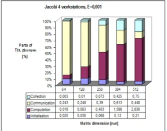
This figure illustrates continually percent spreading of the individual overheads (Initialization, computation, communication, gathering) for Jacobi parallel algorithm with the given number of workstations p = 4 for various values of workload n (matrix dimensions) and for accuracy E=0,001. From comparisons we can see raising trend of computation in dependence of accuracy E.

Generally for the problems with increasing

communication complexity through using great number of processors p based on Ethernet NOW we come to the point (Threshold that parallel computing is no more effective, that means we are without any speed-up. It is evident that for the given problem, given parallel algorithms and given parallel computer to find such a threshold (no speed-up) is very important.

The individual parts of the whole execution parallel time are illustrated at Fig. 15 for Jacobi iterative parallel algorithm for 4 workstations and for E = 0,001.

Figure 15. Percentage comparison of T (s, p)complex for its components (E=0,001).

Figure 16. Comparison of T (s, p)complex parts for p=4 (E=0,001).

n=256

0 50 100 150 200 250 300 350 400 450 500

0 20 40 60 80 100 120 140 160 180 200 220 240 260

p T

[µs]

D1 D2

n=128, 256

0 2 4 6 8 10 12 14 16

9 29 49 69 89 109 129 149 169 189 209 229 249

p ts

[µs]

The influence of number of workstations at given accuracy E=0,001 to the individual parts of the whole solving time for pre Jacobi iterative parallel algorithm for various sizes of input workload (matrix dimensions from 64 x 64 to the size 512 x 512) illustrates Fig. 16 for the number of workstations p = 4. From the comparisons come out percent sinking of computations at the bigger number of workstations (parallel speed-up though the higher number of workstations) at the moderate percent raising of network communication overheads.

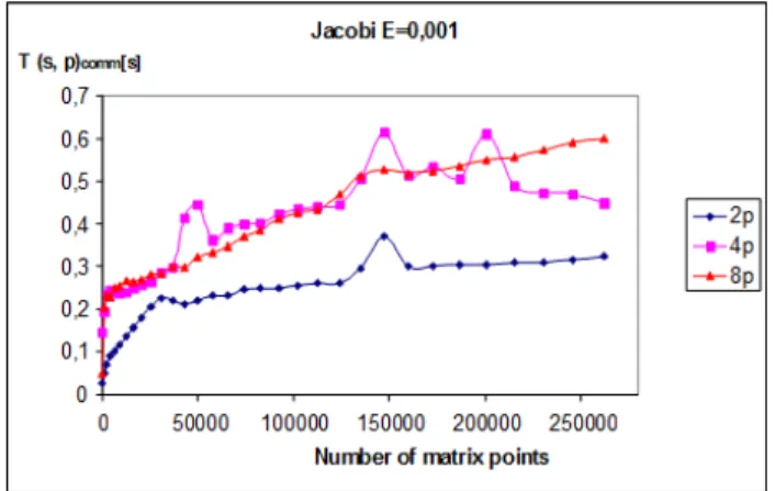
Fig. 17 illustrates the times of individual parts of the whole solving time as a function of input workload n (Square matrix dimensions) for number of workstations p=4 and for accuracy E=0,001. From comparison of these both graphs comes out higher contribution through the number of working stations than the raising overheads of the network communication.

Figure 17. Influence of computing nodes to T(s, p)comm, (E=0,001).

Fig. 18 illustrate influence of number of workstations NOW to quicker solutions of both distributed parallel algorithms (Gauss-Seidel parallel algorithm) for matrix dimensions 512x512 and various analyzed accuracies of Epsilon.

Figure 18. Influence of workstation number for Gauss-Seidel IPA.

Derived analytical issoeficiency functions allow us to predict parallel computer performance also for theoretical not existed ones. We have illustrated at Fig. 19

isoefficiency functions for individual constant values of efficiency (E = 0,1 to 0,9) for n < 152 using the published technical parameters tc, ts, tw communication constants of

used NOW (tc= 0,021 µs, ts = 35 µs, tw= 0,23 µs,).

Figure 19. Isoefficiency functions w(s) for n < 152

Fig. 20 illustrates isoefficiency functions for individual constant values of efficiency (E = 0,1 to 0,9) for n = 1024 and for communication parameters of parallel computer Cray T3E (tc= 0,011µs, ts = 3 µs, tw= 0,063 µs,).

Figure 20. Isoefficiency functions w(s) (n = 1024).

From both pictures (Fig. 19 and Fig. 20) we can see that to keep a given value of efficiency we need step by step increasing number of computing processors and higher value of workload (useful computation) to balance higher communication overheads.

7. Conclusions

Performance evaluation as a discipline has repeatedly proved to be critical for design and successful use in parallel computing. At the early stage of design, performance models can be used to project the system scalability and evaluate alternative solutions. At the production stage, performance evaluation methodologies

0,0E+00 5,0E+06 1,0E+07 1,5E+07 2,0E+07 2,5E+07

0 200 400 600 800 1000

p w

E=0,1

E=0,2

E=0,3

E=0,4

E=0,5

E=0,6

E=0,7

E=0,8

E=0,9

0,0E+00 2,0E+06 4,0E+06 6,0E+06 8,0E+06 1,0E+07 1,2E+07 1,4E+07 1,6E+07 1,8E+07 2,0E+07

0 200 400 600 800 1000

p w

E=0,1

E=0,2

E=0,3

E=0,4

E=0,5

E=0,6

E=0,7

E=0,8

can be used to detect bottlenecks and subsequently suggests ways to alleviate them. Queuing networks has been established in modeling of parallel computers [5, 17]. Extensions of complexity theory to parallel computing have been successfully used for the evaluation of parallel algorithms and communication complexity too. Via extended form of isoefficiency concept for parallel algorithms we have demonstrated its applied using to performance prediction in typical matrix parallel algorithms (MPA).

To derive isoefficiency function in analytical way it is necessary to derive al typical used criterion for performance evaluation of parallel algorithms including their overhead function (parallel execution time, speed up, efficiency). Based on this knowledge we are able to derive issoefficiency function as real criterion to evaluate and predict performance of parallel algorithms also for future hypothetical parallel computers. So in this way we can say that this process includes complex performance evaluation including performance prediction.

Due to the dominant using of parallel computers based on NOW modules and their high integration named as Grid there has been great interest in performance prediction of parallel algorithms in order to achieve effective parallel algorithms (optimized). Therefore this paper summarizes the used methods for complexity analysis which can be applicable to all types of parallel computers (supercomputer, NOW, Grid).

This paper finalizes applying of complex analytical modeling to the whole group of matrix parallel algorithms which are characterized by domain decomposition models. To present this group of MPA we have modeled abstract matrix using basic decomposition models with supposed intensive communication complexity. In such a way performed complex modeling could be inspiring also to other PA or even a group of PA. The complex analyzed examples we have been evaluated so on classic massive supercomputers (hypercube, mesh) as on dominant parallel computers represented by NOW module.

Acknowledgements

This work was done within the project “Complex performance modeling, optimization and prediction of parallel computers and algorithms” at University of Zilina, Slovakia. The author gratefully acknowledges help of project supervisor Prof. Ing. Ivan Hanuliak, PhD.

References

[1] Arora S., Barak B., Computational complexity - A modern Approach, Cambridge University Press, pp. 573, 2009

[2] Bahi J. H., Contasst-Vivier S., Couturier R., Parallel Iterative algorithms: From Sequential to Grid Computing, CRC Press, USA, 2007

[3] Bronson R., Costa G. B., Saccoman J. T., Linear Algebra -

Algorithms, Applications, and Techniques, 3rd Edition, Elsevier Science & Technology, Netherland, pp. 536, 2014

[4] Casanova H., Legrand A., Robert Y., Parallel algorithms, CRC Press, USA, 2008

[5] Dattatreya G. R., Performance analysis of queuing and computer network, University of Texas, Dallas, USA, pp.472, 2008

[6] Davis T. A., Direct methods for sparse Linear Systems, Cambridge University Press, United Kingdom, pp. 184, 2006

[7] Desel J., Esperza J., Free Choise Petri Nets, Cambridge University Press, United Kingdom, pp. 256, 2005

[8] Dubois M., Annavaram M., Stenstrom P., Parallel Computer Organization and Design, Cambridge university press, United Kingdom, pp. 560, 2012

[9] Dubhash D.P., Panconesi A., Concentration of measure for the analysis of randomized algorithms, Cambridge University Press, United Kingdom, 2009

[10] Edmonds J., How to think about algorithms, Cambridge University Press, United Kingdom, pp. 472, 2010

[11] Gelenbe E., Analysis and synthesis of computer systems, Imperial College Press, pp. 324,2010

[12] Goldreich O., P, NP, and NP - Completeness, Cambridge University Press, United Kingdom, pp. 214, 2010

[13] Hager G., Wellein G., Introduction to High Performance Computing for Scientists and Engineers, CRC Press, USA, pp. 356, 2010

[14] Hanuliak P., Hanuliak J., Complex performance modeling of parallel algorithms , American J. of Networks and Communication, Science PG, Vol. 3, USA, 2014

[15] Hanuliak M., Modeling of parallel computers based on network of computing nodes, American J. of Networks and Communication, Science PG, Vol. 3, USA, 2014

[16] Hanuliak M., Hanuliak J., Decomposition models of parallel algorithms, American J. of Networks and Communication, Science PG, Vol. 3, USA, 2014

[17] Hanuliak M., Hanuliak I., To the correction of analytical models for computer based communication systems, Kybernetes, Vol. 35, No. 9, UK, pp. 1492-1504, 2006

[18] Hanuliak J., Modeling of communication complexity in parallel computing, American J. of Networks and Communication, Science PG, Vol. 3, USA, 2014

[19] Hanuliak M., Unified analytical models in parallel and distributed computing, AJNC (Am. J. of Networks and Comm.), SciencePG, Vol. 3, No. 1, USA, pp. 1-12, 2014

[20] Hanuliak J., Hanuliak I., To performance evaluation of distributed parallel algorithms, Kybernetes, Volume 34, No. 9/10, United Kingdom, pp. 1633-1650, 2005

[21] Hillston J., A Compositional Approach to Performance Modeling, University of Edinburg, Cambridge University Press, United Kingdom, pp. 172 pages, 2005

[23] Kshemkalyani A. D., Singhal M., Distributed Computing, University of Illinois, Cambridge University Press, United Kingdom, pp. 756 pages, 2011

[24] Kirk D. B., Hwu W. W., Programming massively parallel processors, Morgan Kaufmann, USA, pp. 280, 2010

[25] Kostin A., Ilushechkina L., Modeling and simulation of distributed systems, Imperial College Press, United Kingdom, pp. 440, 2010,

[26] Kshemkalyani A. D., Singhal M., Distributed Computing, University of Illinois, Cambridge University Press, UK, pp. 756, 2011

[27] Kushilevitz E., Nissan N., Communication Complexity, Cambridge University Press, United Kingdom, pp. 208, 2006,

[28] Le Boudec Jean-Yves, Performance evaluation of computer and communication systems, CRC Press, USA, pp. 300, 2011

[29] Levesque John, High Performance Computing: Programming and applications, CRC Press, USA, pp. 244, 2010

[30] Lilja D. J., Measuring Computer Performance, University of Minnesota, Cambridge University Press, United Kingdom, pp. 280, 2005

[31] McCabe J., D., Network analysis, architecture, and design (3rd edition), Elsevier/ Morgan Kaufmann, USA, pp. 496, 2010

[32] Meerschaert M., Mathematical modeling (4-th edition), Elsevier, pp. 384, 2013

[33] Misra Ch. S.,Woungang I., Selected topics in communication network and distributed systems, Imperial college press, United Kingdom, pp. 808, United Kingdom

[34] Peterson L. L., Davie B. C., Computer networks – a system approach, Morgan Kaufmann, USA, pp. 920, 2011

[35] Resch M. M., Supercomputers in Grids, Int. J. of Grid and HPC, No.1, pp. 1 - 9, 2009

[36] Riano l., McGinity T.M., Quantifying the role of complexity in a system´s performance, Evolving Systems, Springer Verlag, Germany, pp. 189 – 198, 2011

[37] Shapira Y., Solving PDEs in C++ - Numerical Methods in a Unified Object-Oriented Approach (2nd edition), Cambridge University Press, United Kingdom, pp. 800, 2012

[38] Wang L., Jie Wei., Chen J., Grid Computing: Infrastructure, Service, and Application, CRC Press, USA, 2009 www pages