Decomposition Models of Parallel Algorithms

Published online July 30, 2014 (http://www.sciencepublishinggroup.com/j/ajnc) doi: 10.11648/j.ajnc.s.2014030501.16

ISSN: 2326-893X (Print); ISSN: 2326-8964 (Online)

Decomposition models of parallel algorithms

Michal Hanuliak, Juraj Hanuliak

Dubnica Technical Institute, Sladkovicova 533/20, Dubnica nad Vahom, 018 41, Slovakia

Email address:

[email protected] (M. Hanuliak)

To cite this article:

Michal Hanuliak, Juraj Hanuliak. Decomposition Models of Parallel Algorithms. American Journal of Networks and Communications. Special Issue: Parallel Computer and Parallel Algorithms. Vol. 3, No. 5-1, 2014, pp. 70-84. doi: 10.11648/j.ajnc.s.2014030501.16

Abstract:

The article is devoted to the important role of decomposition strategy in parallel computing (parallel computers, parallel algorithms). The influence of decomposition model to performance in parallel computing we have illustrated on the chosen illustrative examples and that are parallel algorithms (PA) for numerical integration and matrix multiplication. On the basis of the done analysis of the used parallel computers in the world these are divided to the two basic groups which are from the programmer-developer point of view very different. They are also introduced the typical principal structures for both these groups of parallel computers and also their models. The paper then in an illustrative way describes the development of concrete parallel algorithm for matrix multiplication on various parallel systems. For each individual practical implementation of matrix multiplication there is introduced the derivation of its calculation complexity. The described individual ways of developing parallel matrix multiplication and their implementations are compared, analyzed and discussed from sight of programmer-developer and user in order to show the very important role of decomposition strategies mainly at the class of asynchronous parallel computers.

Keywords:

Parallel Computer, Parallel Algorithms, Performance, Decomposition Model, Numerical Integration, Matrix Multiplication

1. Parallel Computing

Performance of actually computers (sequential, parallel) depends from a degree of embedded parallel principles on various levels of technical (hardware) and program support means (software). At the level of intern architecture of basic module CPU (Central processor unit) of PC they are implementations of scalar pipeline execution or multiple pipeline (superscalar, super pipeline) execution and capacity extension of cashes and their redundant using at various levels and that in a form of shared and local cashes (L1, L2, L3). On the level of motherboard there is a multiple using of cores and processors in building multicore or multiprocessors system as SMP (symmetrical multiprocessor system) as powerful computation node, where such computation node is SMP parallel computer too [1]. On the level of individual computers the dominant trend is to use multiple number of high performed workstations based on single personal computers (PC) or SMP, which are connected in the network of workstations (NOW) or in a high integrated way named as Grid systems [36]. A member of NOW or Grid could be any classic supercomputers [34].

1.1. Parallel Computers

From the point of system programmer we can divide all to this time realized parallel computers. The basic classification is from the point of realized memory as follows

• parallel computers with shared memory

(multiprocessors, multicores)

• parallel computers with distributed memory (mainly based on computer networks)

• others.

1.1.1. Parallel Computers with Shared Memory Basic common characteristics are as following [8, 13] • shared memory

• using shared memory for communication • supported developing standard

OpenMP

OpenMP Threads Java

• typical architectures [37]

Grid

meta computers others.

1.1.2. Parallel Computers with Distributed Memory Basic common characteristics are as following [22, 33] • no shared memory (distributed memory)

• computing node could have some form of local memory where this memory in use only by connected computing node

• cooperation and control of parallel processes only using asynchronous message communication • supported developing standard

MPI (Message passing interface) PVM (Parallel virtual machine) Java

• typical architectures

network of workstations (NOW) Grid

meta computers others.

2. Parallel Algorithms

Description (diagram)

Sequential algorithm

Way of computing

Problem

Parallel

Analyst Abstract formalization

Practice

Aplication informatics

Accuracy of solving Sequential

No

Complex algorithm

End

No Parallel

algorithm

Accuracy of solving

No Modification of algorithm

Modification of algorithm

Yes Expert to

problem

Figure 1. Deriving process of parallel algorithm.

Users and programmers from a beginning of applied computer using request more powerful computers and more efficient applied algorithms. For a long time to effective technologies belong implementations of parallel principles so into computers as applied parallel algorithms. In this way term parallel programming could relate to every program, which contains more than one parallel process [21, 23]. This process represents single independent sequential part of program. Basic attribute of parallel algorithms is to

achieve faster solution in comparison to quickest sequential solution. The role of programmer is for the given parallel computer and for the given application task to develop parallel algorithm (PA). Fig. 1 demonstrates how to derive parallel algorithm from existed sequential algorithms.

In last year’s there is increased interest of scientific research into effective parallel algorithms. These trends to parallel algorithms also support actual trends in programming technologies to the development of modular applied algorithms based on object oriented programming (OOP). OOP algorithms are in their merits result of abstract thinking toward parallel solutions for existed complex problems.

2.1. General Classification of Parallel Algorithms

In general we supposed that potential effective parallel algorithms according defined algorithm classification (Fig. 2) should be in the group P as classified polynomial algorithms.

NP

NPC NC

P

PC

Figure 2. Parallel algorithm classification.

Other used acronyms at Fig. 2 are as following [12] • NP – general non polynomial group of all algorithms • NC (Nick´s group). Group of effective polynomial

algorithms

• PC – polynomial complete. Group of polynomial algorithms with high complexity

• NPC – non polynomial complete. This group consists of non-polynomial algorithms with their high solving complexity. The existence of any NPC algorithm in an effective way makes it available to solve effective also other NPC algorithms.

2.2. Parallel Processes

To derive PA we have to create conditions for potential parallel activities through dividing the input problem algorithm to its independent parts (decomposition model) according Fig. 3. These individual parts could be as following

• heavy parallel processes

Complex p

( )

roblem sequential algorithm

Decomposition

Parallel proces s n Parallel

proces 2s Parallel

proces 1s . . .

Figure 3. Illustration of decomposition process.

We will define standard process as developed sequential algorithm or its independent part. In detail standard process does not represent only some part of compiled program because to its characterization belongs also register status of processor. Illustration of such standard process is at Fig. 4.

Figure 4. Illustration of standard process.

Every standard process has therefore own system stack, which contains process local data and in case of process interruption also actual register status of processor. It is obvious that we may have contemporary multiple numbers of standard processes, which used together some program part but their processes contexts (process local data) are different. Needed tools to manage processes (initialization, abort, synchronization, communication etc.) are within cores of multitask operation systems in form of services. Illustration of standard multi processes state is at Fig. 5.

Figure 5. Parallel algorithm based on multiple parallel processes.

But concept of generating standard processes with individual address spaces is very time consuming. For example in operation system UNIX a new process is generating with operation fork(), which makes system call in order to create child process with new own address space. But in detail it means memory allocation, copying of data segment and descriptor of origin (parent) process and realization of child process stack. Therefore this concept we named as heavy-weighted process. It is obvious that heavy-weighted approach does not support effectiveness of applied parallel processing and needed scalability of parallel algorithms. In relation to it were necessary to develop another less time consuming concept of process generation named as light-weighted process. This lighten conception of generating new processes under another name as threads were implemented at various operation systems, supported threads libraries and parallel developing environments. Basic difference between standard process and thread is that we can within standard process generate additional new threads, which are together using the same address space including descriptor declaration of origin standard process.

2.3. Parallel Algorithms Classification

In principal parallel algorithms are dividing into two following basic classes

• parallel algorithms with shared memory (PAsm). In this

case parallel processes can communicate through shared variables using existed shared memory. For control of parallel processes are used typical synchronization tools as busy waiting, semaphores and monitors to guarantee exclusive using of shared resources only by single parallel process [10, 28]

• parallel algorithms with distributed memory (PAdm).

Distributed parallel algorithms have to

synchronization and cooperation of parallel processes only network communication. The term distributed (asynchronous) parallel algorithms defines, that individual parallel processes are performed on independent computing nodes of used parallel computer with distributed memory [16, 31]

• mixed PA. Very perspective parallel algorithms which are to use advantages of dominant parallel computers based on NOW modules as following

using of parallel processes with shared memory in individual computing nodes of parallel computer

using of parallel processes based on distributed memory in parallel computers with distributed memory.

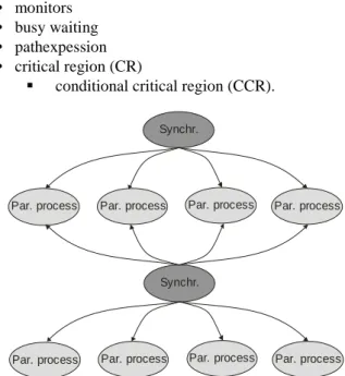
2.3.1. Parallel Algorithms with Shared Memory

Typical activity graph of parallel algorithms with shared memory PAsm is at Fig. 6. To control decomposed parallel

processes there is necessary synchronization mechanism as follows

• monitors • busy waiting • pathexpession • critical region (CR)

conditional critical region (CCR).

S nchr.y

Par. process Par. process Par. process Par. process

S nchr.y

Par. process Par. process Par. process Par. process

Figure 6. Illustration of parallel activities of PAsm.

2.3.2. Parallel Algorithms with Distributed Memory

Parallel algorithms with distributed memory PAdm are

parallel processes which are performing on asynchronous computing nodes of given parallel computer. Therefore for all needed cooperation of parallel processes we have available only inter process communication IPC. The principal illustration of parallel processes for PAdm is at Fig.

7.

Par.

process . . .

Par. process

Par. process

Par. process

Figure 7. Illustration of parallel activities of PAdm.

3. The Role of Performance in Parallel

Computing

Quantitative evaluation and modeling of hardware and software components of parallel systems are critical for the delivery of high performance. Performance studies apply to initial design phases as well as to procurement, tuning and capacity planning analysis. As performance cannot be expressed by quantities independent of the system workload, the quantitative characterization of resource demands of application and of their behavior is an important part of any performance evaluation study [6, 27]. Among the goals of parallel systems performance analysis are to assess the performance of a system or a system component or an application, to investigate the match

between requirements and system architecture

characteristics, to identify the features that have a significant impact on the application execution time, to predict the performance of a particular application on a given parallel system, to evaluate different structures of

parallel applications. In order to extend the applicability of analytical techniques to the parallel processing domain, various enhancements have been introduced to model phenomena such as simultaneous resource possession, fork and join mechanism, blocking and synchronization. Modeling techniques allow to model contention both at hardware and software levels by combining approximate solutions and analytical methods. However, the complexity of parallel systems and algorithms limit the applicability of these techniques. Therefore, in spite of its computation and time requirements, simulation is extensively used as it imposes no constraints on modeling.

3.1. The Role of Performance in Parallel Computing

To the performance evaluation in parallel computing we briefly review the techniques most commonly adopted for the evaluation in parallel computing as follows

• analytical

application of queuing theory results [11, 20] order (asymptotic) analysis [3, 15]

Petri nets [7] • simulation methods [24] • experimental

benchmarks [32] direct measuring [9, 29].

Analytical method is a very well developed set of techniques which can provide exact solutions very quickly, but only for a very restricted class of models. For more general models it is often possible to obtain approximate results significantly more quickly than when using simulation, although the accuracy of these results may be difficult to determine.

Simulation is the most general and versatile means of modeling systems for performance estimation. It has many uses, but its results are usually only approximations to the exact answer and the price of increased accuracy is much longer execution times. They are still only applicable to a restricted class of models (though not as restricted as analytic approaches.) Many approaches increase rapidly their memory and time requirements as the size of the model increases.

Evaluating system performance via experimental measurements is a very useful alternative for computer systems. Measurements can be gathered on existing systems by means of benchmark applications that aim at stressing specific aspects of computers systems. Even though benchmarks can be used in all types of performance studies, their main field of application is competitive procurement and performance assessment of existing systems and algorithms.

3.2. Performance Evaluation Metrics of Decomposition Models

• parallel execution time T(s, p) as the execution time performed by p computing nodes (processors, cores, workstations) of given parallel computer and s defines input size (load) of given problem

• speed up factor S(s, p) as

) , (

) 1 , ( ) , (

p s T

s T p s

S =

• efficiency E(s, p) as

) , (

) 1 , ( ) , ( ) , (

p s T p

s T p

p s S p s

E = =

• the isoefficiency concept

).

,

(

1

)

(

h

s

p

E

E

s

w

−

=

4. Developing Process of Parallel

Algorithms

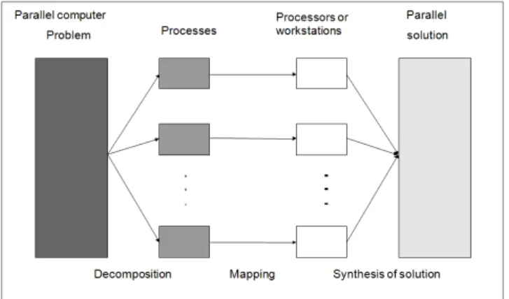
To exploit the parallel processing capability the application program must be parallelized. The effective way how to do it for a particular application problem (decomposition model) belongs to the most important step in developing an effective parallel algorithm [14, 18]. The development of the parallel network algorithm according Fig. 8 includes the developing activities as follow

• decomposition - the division of the application into a set of parallel processes

• mapping - the way how processes and data are distributed among the nodes

• inter process communication - the way of

corresponding and synchronization among individual processes

• tuning - alternation of the working application to improve performance (performance optimization).

Figure 8. Development steps in parallel algorithms.

To do these steps there is necessary to understand the concrete application problem, the data domain, the used algorithm and the flow of control in given application. When designing a parallel program the description of the high level algorithm must include, in addition to design a sequential program, the method you intend to use to break the application into processes or threads (decomposition

model) and distribute data to different nodes (mapping). The chosen decomposition model drives the rest of program development.

4.1. Decomposition Models

Developing of sequential algorithms implicitly supposed existence of algorithm for given problem. Only later in stage of practical programming they are defined and used suitable data structures. In contrast to this classic developing method suggestion of parallel algorithm should include at beginning stage potential decomposition strategy including distribution of input data to perform decomposed parallel processes. Selection of suitable decomposition strategy has cardinal influence to further development of parallel algorithm.

Decomposition strategy defines potential dividing of given complex problem to their independent parts (Parallel processes) in such a way, that they could be performed in a parallel way through computing nodes of given parallel computer. Existence of some decomposition method is critical assumption to possible parallel algorithm. Potential decomposition degree of given complex problem is crucial for effectivity of parallel algorithm [4, 17]. To this time

developed parallel algorithms and corresponding

decomposition strategies were mainly related to available synchronous parallel computers based on classic massive parallel computers (supercomputers and their innovations). Developing parallel algorithms for actual dominant parallel computers NOW and Grid require at least modified decomposition strategies incorporating following priorities

• emphasis to functional parallelism of complex problems

• minimization of inter process communication IPC. The most important step is to choose the best decomposition model for given complex problem. To do this it is necessary to understand concrete application problem, data domain, used algorithm and flow of control in given complex problem. When designing a parallel program the description of the high-level algorithm must include, in addition to design a sequential program, the method you intend to use to break the application into processes and distribute data to different computing nodes. The chosen decomposition models drive the rest of PA development. This is true is in case of developing new application as in porting serial code. The decomposition method tells us how to structure the code and data and defines the communication topology [25, 26].

(classic parallel computers). On other way the realization of PA for in this time dominate parallel computers (SMP, NOW, Grid) demand modified decomposition models and strategies with respect to minimization of interposes communication intensity (NOW, Grid) and deriving waiting

latency T(s, p)wait at using shared resources or at

insufficient their capacities

• naturally parallel decomposition • domain decomposition

• control decomposition manager/workers functional

• divide-and-conquer strategy for • decomposition of big problems • object oriented programming (OOP).

4.1.1. Natural Parallel Decomposition

Natural parallel decomposition allows simple creating of parallel processes whereby to their cooperation normally there is necessary low amount of inter process communication IPC. Also for parallel computation there is normally not important sequence of individual solutions. As a consequence there are not necessary any synchronization of performed parallel processes during parallel computation. Based on these attributes natural parallel algorithms allows to achieve practical ideal p - multiple speed - up using p - computation nodes of parallel computer (linear speed – up), and that with minimal additional efforts at developing parallel algorithms. Typical examples are numerical integration parallel algorithms. Based on this example we will illustrate in detail the role of decomposition models in developing steps of parallel algorithms.

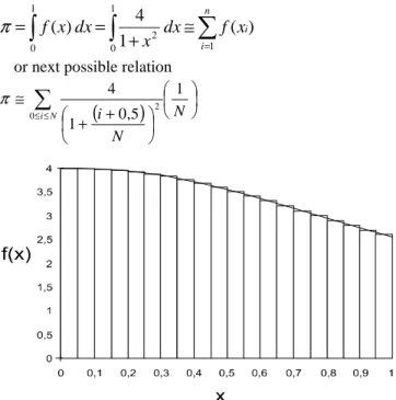
4.1.1.1. Numerical Integration

Numerical integration algorithms are typical examples with implicitly latent decomposition strategy in which the parallelism is the integral part of own algorithm. Standard way of typical numerical integration algorithm (the

computation of π number) assumes that we divide the

interval <0, 1> to n identical subintervals whereby in each subinterval we approximate its part of curve with rectangle. Function values in middle of each subinterval determine height of the rectangle. Number of selected subintervals

determines computation accuracy. The computed value of π

will be given as sum of surface area of defined individual

approximated rectangles. Illustration of numerical

integration applied to π computation is at Fig. 9. Concretely

for the calculation of the value π the following standard formula is used

∫

₊

=

1

0 2

1

4

dx

x

π

, where h = 1 / n is the width of the selected splitting

interval, xi = h (i - 0.5) are mid-ranges and n is the number

of selected intervals (accuracy). For computation of π we can use an alternative following interpolating polynomial [93]

∑

∫

∫

=

≅

+

=

=

n

i i

x

f

dx

x

dx

x

f

1 1

0 2 1

0

)

(

1

4

)

(

π

or next possible relation

(

)



       



 ₊ +

≅

∑

≤

≤ N

N i

N i

1

5 , 0 1

4

0 2

π

Figure 9. Principle of numerical integration.

4.1.1.2. Decomposition Model

For the parallel way of numerical integration computation we are used the property of latent decomposition strategy in all natural parallel algorithms. We divide the whole needed computation to its individual parallel processes according to the Fig. 10 where are for simplicity illustrated four parallel processes. For the

parallel computation of number π we then use these created

parallel processes.

0 0,5 1 1,5 2 2,5 3 3,5 4

f(x)

x

0 1 2 3 0 1 2 3 0 1 2 3 0 1 2 3 0 1 2 3

Figure 10. Decomposition model of numerical integration problems.

enter the desired number of subintervals n compute the width w of each subinterval for each subinterval

find its centre x

compute f(x) and the sum end of cycle

The prospective parallel implementations on dominant parallel computers (SMP, NOW, Grid) allow analysis of communication load depending on input computation load because input load is proportional to changes in load communication.

4.1.1.3. Mapping of Parallel Processes

The individual independent processes we distribute forcomputation in such way that every created parallel process will be executed on different computing node of parallel computer (mapping). After the parallel computation in individual nodes of a network of workstations was performed we need only to sum the partial results to get final result. To manage this task we have to choose one of the computing nodes to handle it. As well at the computation begin the chosen node (let it be node 0) must know the value of n (number of the strips in every process) and then selected node 0 has to let it know to all other computing nodes. Example of the parallel computation algorithm (manager process) is then as following

if my node is 0

read the number n of strips desired and send it to all other nodes

else

receive n from node 0 end if

for each strip assigned to this node

compute the height of rectangle (at midpoint) and sum result

end for

if my node is not 0

send sum of result to node 0 else

receive results from all nodes and sum

multiple the sum by the width of the strips to get π return

Sending values of n / p could be done in case of parallel

algorithm with distributed memory PAdm using MPI API

explained collective communication command Broadcast in case of the same size of parallel processes or MPI command Scatter in case of variable size of parallel processes.

We illustrate on this relative simple example parallel algorithm in parallel language FORTRAN for parallel computer with distributed memory. The algorithm extends and modifies the starting serial algorithm for the specific parallel implementation. To characterize shortly this parallel algorithm, we note that number of computing nodes of a parallel computer and identification of each computing node performed procedures numnodes() (number of computing nodes), mynode() (my computing node) and my pid() (number of my parallel process). These procedures allow the activation of any number of computing nodes of a parallel system. Then if we allow designated node, for example computing node 0, perform

management functions and certain partial computations, while other nodes perform a substantial part of the rest of computations for assigned subintervals, and communicated obtained partial amounts specified computing node 0. Procedures silence and crecv serve to ensure the required collective data communications and the final summation of achieved partial results.

f(x) = 4.0 /(1.0 + x*x) integer n, i, p, me, mpid real w, x, sum, pi

p = numnodes () return number of nodes me = mynode () return number of my node mpid = mypid () return id of my process msglen = 4 estimate message length allnds = -1 message name for all nodes msgtp0 = 0 name for message 0 msgtp1 = 1 name for message 1 if (me .eg. 0) then if i am node 0

read *, n read number of subintervals n callcsend (msgtp0,n,msglen,allnds,mpid) and send it to all other nodes

else if I am any other node callcrecv (msgtp0, n, msglen) receive value n end if

w = 1.0/n sum = 0.0

do 10 i = me+1, n dividing subintervals among nodes x =w*(i-0.5)

sum = sum + f(x) 10 continue if (me .ne. 0) then if I am not node 0

callcsend (msgtp1, sum, 4, 0, mpid) send partial result to node 0

else if I am node 0

do 20 i = 1, p-1 for every other used node callcrecv (msgtp1, temp, 4) receive partial result to temp

sum = sum + temp and add it to sum 20 continue

pi = w*sum compute final result

print *,pi and print it endif

end

The disadvantage is that the implementation of the central necessary routing communications through the designated node 0 (manager node), and as a result there may be a bottleneck which could negatively affect the efficiency of the parallel algorithm implementation.

4.1.1.4. Performance Optimization

very important to minimize the number of communicating data messages proportionally to number of computational operations, thereby minimizing also overall execution time

of a parallel algorithm. In computation of number π

demanded centralization of needed communication through manager computing node 0 may come to computation bottleneck for two following reasons

• manager computing node 0 node could simultaneously receive data message only from one other computation node

• summary of the partial results at manager node 0 is done sequentially, in a sequential way, which is just a prerequisite to come to bottleneck.

The outgoing point in mentioned both cases is to consider using of collective communication commands of standardized development environments as MPI API, and that collective command Reduce or Gather. For some parallel computers are available alternative global summarization operation gssum(), just to eliminate such bottlenecks. This operation in iterative manner always sums partial results of two computing nodes, which both computing nodes are exchanged. Each partial sum, which receives one of computing node pair, is added to the obtained sum in a given node, and this result is transmitted to next computing node of defined communication chain. In this way there is gradually obtained the total accumulated amount of the computing nodes whereby manager computing node 0 can perform the last sum and print the final result. This procedure of global summarization can be also programmed, but the sequence

of implemented appropriate procedures simplifies

implementation of parallel algorithms and contributes to its effectiveness too.

In other applied tasks using a larger direct inter process communication implementation of communication used, for example form of asynchronous communication using direct support of multitasking in a given node, thereby achieving parallelism implementation of communication activities other node. Of course, an example of reducing the ratio of communication computing activity is not the only task in optimizing the performance of parallel algorithms. Available methods for optimizing performance are virtually the same colorful as diverse mere parallel application tasks. Inspired examples and procedures will therefore be included in the illustrative application examples in the following sections. Commonly used method and procedure for the decomposition of the application tasks indirectly implies the possibilities of optimizing its performance, i.e., optimization can also cause re-evaluation of strategies used decomposition.

Then if we allow designated node, for example node 0, perform management functions and certain partial calculations while other nodes perform a substantial part of

the calculations for assigned subintervals, and

communicate obtained partial amounts to specified node 0. Procedures silence and crecv serve to ensure the required communication.

It is also important to note that for mentioned module is required direct communication of every computing node with other computing nodes as assumption of parallel communication between multiple pairs of computing nodes. In this approach the final sum can be obtained after performing the second, third or even fourth cycle of the

communication chain. In fact we need only log2 p, where p

is the number of computing nodes of parallel computer, cycles of communication chains compared to n data messages at initial implementation. Used parallelism of data message exchange will therefore increase efficiency of parallel algorithms. For the implementation of an improved approach for data messages communications it’s necessary to replace following part

if (me .ne. 0) then

callcsend (msgtp1, sum, msglen, 0, mpid) else

do 20 i = 1, p-1

callcrecv (msgtp1, temp, msglen) sum = sum + temp

20 continue pi = w*sum print *, pi endif end

with next part

callgssum (sum, 1, temp) if (me .eg. 0) then pi = w*sum print *, pi endif

In other applied parallel algorithms there is possible at using a larger direct inter process communication to perform communication for example in form of asynchronous communication using multitasking support in a given node, thereby it is achieved parallelism of performing communication with other computing node activity. Of course described example of reducing ratio of communication/ computing activity is not the only task in optimizing the performance of parallel algorithms. Available methods for performance optimizing are practical so various as are diverse parallel application problems.

4.1.2. Domain Decomposition

These both matrix parallel algorithms we have chosen to represent typical examples of matrix data decomposition models.

4.1.2.1. Decomposition Methods for Matrix Multiplication We will illustrate the role of optimal selection of decomposition model on matrix multiplication. The principle of matrix multiplication we illustrate for simplicity for the matrixes A, B with numbers of rows and columns k=2. The result matrix C = A x B is

The way of sequential calculation is following Step 1:

compute all the values of the result matrix C for the first row of matrix A and for all columns of the matrix B Step 2 :

take the next row of matrix A and repeat step 1.

In this procedure we can see the potential possibility of parallel computation that is the repetition of activities in the step 1 always with another row of matrix A. Let consider the calculation example of matrix multiplication on parallel system. The basic idea of the possible decomposition procedure illustrates Fig. 11.

Figure 11. Standard decomposition of matrix multiplication.

The procedure is as following Step 1:

give to the i-th node horizontal column of the matrix A with their names A´i and i-th vertical column of the

matrix B named as B´i

Step 2:

compute all values of the result matrix C for A´i and B´i

and named them as C´ii

Step 3:

give to i-th computing node its value B´i to the node i-1

and get B´i+1 value from computing node i+1.

Repeat the steps 2 and 3 to the time till i-th node does

not computed C´i,i-1 values with B´i-1 columns and row A´i.

Then i-th node computed i-th row of the matrix C (Fig. 12.) for the matrix B with the number k-columns. The advantage of such chosen decomposition is the minimal consume of memory cells. Every node has only three values (rows and columns) from every matrix.

Figure 12. Illustration of the gradually calculation of matrix C.

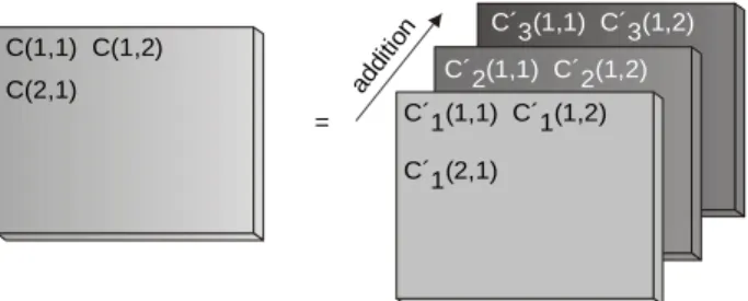
This method is also faster as second possible way of decomposition according Fig. 13.

Figure 13. Matrix decomposition model with columns of first matrix.

The procedure is following Step 1:

give to the i-th node vertical column of the matrix A (A´i)

and the horizontal row of the matrix B (B´i).

Step 2:

perform the ordinary matrix computation A´i and B´i.

The result is the matrix C´i of type n x n. Every element

from C´i is the particular element of the total sum which

corresponds to the result matrix C. Step 3:

call the function of parallel addition GSSUM for the creating of the result matrix C through corresponded elements C´i. This added function causes increasing of

the calculation time, which strong depends on the magnitude of the input matrixes (Fig. 14.).

Figure 14. Illustration of the gradually calculation of the elements C´i,j.

Let k be the magnitude of the rows or columns A, B and U defines the total number of nodes. Then

. . .       =       ⋅ + ⋅ ⋅ + ⋅ ⋅ + ⋅ ⋅ + ⋅ =       ×       22 21 12 11 22 22 12 21 21 22 11 21 22 12 12 11 21 12 11 11 22 21 12 11 22 21 12 11 c c c c b a b a b a b a b a b a b a b a b b b b a a a a

C´_{i , 1}

...

C´_{i , i - 2} C´_{i , i - 1} C´_{i , i} C´_{i , i + 1} C´_{i , i + 2}

...

C´_{i , k}

A´

i ×

B´

i ⇒

C´

= C(1,1) C(1,2)

C(2,1) addi

tion

C´ (1,1) C´ (1,2)

C´ (2,1)

3 3

3

C´ (1,1) C´ (1,2)

C´ (2,1)

2 2

1

C´ (1,1) ₁ C´ (1,2) C´ (2,1)

1 1

( )

( )

k k k k k k

and the finally element of matrix C

4.1.2.2. Decomposition Matrix Models

Any matrix is a regular data structure (domain) for which we can create parallel processes dividing matrix into strips (rows, columns). In generation process of matrix parallel processes there is necessary to tray allocate domain parts in such a way that every computing node has roughly the same number of strips (rows, columns). If the total number of strips is divisible by the number of processors without rest then all computing node will have the same number of decomposed parts (load balance). Otherwise some computing node has some strips extra.

Figure 15. Matching of data blocks.

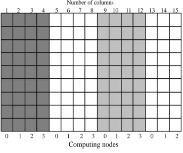
Figure 16. Assigns columns.

Matrix allocation methods of decomposed strips (rows, columns) for solving system of linear equations by Gauss

eliminated method (GEM) are as follows [5] • allocation of block strips

• gradually allocation of strips.

In the first allocation method strips are divided to set of strips and to every computing node is assigned one block. Illustration of these allocation methods is at Fig. 15. At another method with gradual allocation of columns they are allocated columns to individual computing nodes like the card are gradually passing out at games to game participants. Illustration of gradual assignment of columns is at Fig. 16.

4.1.3. Functional Decomposition

Functional decomposition strategies concentrate their attention to find parallelism in distribution of sequential computation stream in order to create independent parallel processes. In comparison to domain decomposition we are concerned to create potential alternative control streams of concrete complex problem. In this way we are streaming in functional decomposition to create so much as possible of parallel threads. Illustration of functional decomposition is at Fig. 17.

Figure 17. Illustration of functional decomposition.

The widely distributed functional strategies are as following

• controlled decomposition

• manager / workers (server / clients).

Typical parallel algorithms are complex optimization problems, which are connected with consecutive searching of massive data structures.

4.1.3.1. Control Decomposition

Control decomposition as an alternative of functional decomposition concentrates to given complex problems as sequence of individual activities (operations, computing steps, control activities etc.), from which we are able to derive multiple control processes. For example we can consider searching tree, which respond to game moves where branch factor is changed from node to node. Any static allocation of tree is not possible or activates

( )

U k U k Mk Mk

U

a

b

a

b

C

′

1

,

1

=

_{1,( −1) +1}

⋅

_{1,( −1) +1}

+

.

.

.

+

_1,

⋅

_1,

( )

∑

( )

=

′

=

U

i i

C

C

1

1

,

1

1

,

1

Number of columns

1 2 3 4 5 6 7 8 9 10 11 12 13 14 15

0 1 2 3 0 1 2 3 0 1 2 3 0 1 2

Computing nodes

Number of columns

1 2 3 4 5 6 7 8 9 10 11 12 13 14 15

0 1 2 3 0 1 2 3 0 1 2 3 0 1 2

unbalanced load.

So in this way this decomposition method supposed irregular structure controlled decomposition which is soft connected with complex problems in artificial intelligence and similar non numerical applications. Secondary it’s very natural to look at any complex problem as collection of modules, which represent needed functional parts of given algorithm.

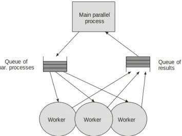
4.1.3.2. Decomposition Strategy Manager / Workers Another alternative of functional decomposition is the strategy manager / workers. In this case there is used one parallel process as control one (manager). Manager process then sequentially and continuously generates needed parallel processes (workers) to their performing in controlled computing nodes. The illustration of parallel structure of decomposition model manager / workers is at Fig. 18. One of the possible applied solutions illustrates Fig. 19.

Main par. process

Worker Worker Worker Worker

Main par. process

Worker Worker Worker Worker

Figure 18. Manager / worker parallel structure.

Manager process controls computation sequence in relation to sequential finishing allocated parallel processes from individual workers. This decomposition strategy is suitable mainly in such cases in which given problem does not content static data or known fixed number of computations. In such cases there is necessary to concentrate to control aspects of individual parts of complex problems. From performed analysis then comes out needed communication sequence to achieve demanded time sequences of created parallel processes. Dividing degree of given complex problem coincide with number of computing nodes of parallel computer, with parallel computer architecture and with performance knowledge of computing nodes. One of important element of previous steps is allocation algorithm. It is more effective to allocate parallel process to first free computing node (worker) in comparison to some defined sequence order of allocation.

Q of

par. processesueue Qresultsueue of

Main parallel process

Worker Worker Worker

Figure 19. Illustration of manager / workers strategy.

4.1.4. Divide and Conquer Decomposition Model

Divide and conquer strategy decomposed complex problem into subtasks of the same size but it iteratively keeps repeating this process to obtain yet smaller parts of given complex problems. In that sense this decomposition model iteratively applies the problem partitioning technique as we can see it at Fig. 20. Divide and conquer is sometimes called recursive partitioning. Typically complex problem size is an integer power of 2 and the divide and conquer strategy halves complex problem into two equal parts at each iteration step.

Figure 20. Illustration of divide and conquer strategy (n=8).

Every from N / 2 – point DFT we can again divide to next parts, that is to two N / 4 – point DFT. Applied decomposition strategy could follows till to exhausting dividing possibility for given N (one point value). Dividing factor is named as radix - q, and that for dividing number higher than two. We have applied decomposition model of divide-and-conquer strategy for parallel solution of fast discrete Fourier transform (DFFT) in [15].

would be useful to apply at every existed level another decomposition model. This approach we are naming as multilayer decomposition.

To effective using of multilayer decomposition contributes new generation of common parallel computers based on implementation of the order more than thousand computing nodes (processors, cores). Secondly unifying trends of high performance parallel computing (HPC) based on massive parallel computers (massive SMP, supercomputers) and distributed computing (NOW, Grid) open to programmers new horizons.

To the typical complex problems belong weather prognosis, fluid flow, structural analysis of substance building, nanotechnologies, high physics energies, artificial intelligence, symbolic processing, knowledge economic etc. Multilayer decomposition model makes it available to decompose complex problem at first to simpler modules and then in second phase to apply suitable decomposition model only to given decomposed part.

4.1.6. Object Oriented Decomposition

Object oriented decomposition is integral part of object oriented programming (OOP). Actually it presents modern way of parallel program development. OOP beside increased demand to abstract thinking of programmer contents decomposition of complex problem to independent parallel modules named as objects [35]. In this way object oriented approach looks at complex problem as collection of abstract data structures (objects), where integral parts of objects are also build object functions as other form of parallel processes. In the same way OOP creates bridge between sequential computers and modern parallel computers based on SMP, NOW and Grid. Illustration of object structure is at Fig. 21.

. . .

Obje t

c

D ta objea ct

Procedure 1

Procedure 2

Procedure n

Figure 21. Object structure.

4.1.7. Mapping

This step allocates created parallel processes to computing nodes of parallel computer for their parallel execution. There is necessary to achieve that every computing node should perform allocated parallel processes (one or more) with at least approximate input

loads (load balancing) on real assumption of equal powerful computing nodes. Fulfillment of this condition contributes to optimal parallel solution latency.

4.1.8. Inter Process Communication

In general we can say that dominated elements of parallel algorithms are their sequential parts (Parallel processes) and analyzed inter process communication (IPC) among performed parallel processes using high speed communication networks [2, 37].

4.1.8.1. Inter Process Communication in Shared Memory Any concrete communication mechanism make use existence of shared memory which allows every parallel process to story communicating data at some addressed memory place and then another parallel process to read stored data (shared variable). It looks very simple but there is necessary to guarantee that in the same time can use the addressed memory place only one parallel process. These needed control mechanism are named as synchronization tools. The typical synchronization tools are as following

• busy waiting • semaphores

• conditional critical regions (CCR) • monitors

• path expressions.

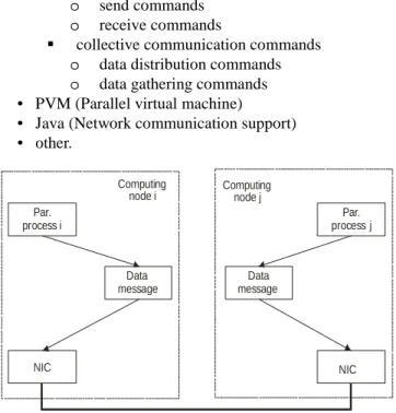
4.1.8.2. Inter Process Communication in Distributed Memory

Inter process communication (IPC) for parallel algorithm

with distributed memory (PAdm) is defined within

supporting developing standards as following • MPI (Message passing interface)

point to point (PTP) communication commands

o send commands

o receive commands

collective communication commands

o data distribution commands

o data gathering commands

• PVM (Parallel virtual machine) • Java (Network communication support) • other.

NIC NIC

Par. process i

Par. process j Computing

node i

communication channel Data

message

Data message Computing

node j

To create needed synchronization tools in MPI we have available only existed network communication of connected computing nodes. Typical MPI network communication is at Fig. 22. Based on existed communication links MPI contains synchronization command Barrier.

4.1.9. Performance Tuning

After verifying developed parallel algorithm on concrete parallel system the further step is performance modeling and optimization (effective PA). This step contents analysis of previous steps in such a way to minimize whole latency of parallel computing T(s, p). Performed optimization of T(s, p) for given parallel algorithm depends mainly from following factors

• allocation of balanced input load to used computing nodes of parallel computer (load balancing) [19] • minimization of accompanying overheads amounts

(parallelization, inter process communication IPC, control of PA) [30].

To do load balancing we need in case of obvious using of equally powerful computing nodes of PC results of load allocation for given developed PA. In dominated asynchronous parallel computers (NOW, Grid) there are necessary to reduce (optimize) mainly number of inter process communications IPC (communication load) for

example through using of alternative existing

decomposition model.

5. Chosen Illustration Results

Figure 23. Computation and communication latencies for epsilon=10-5_.

We illustrate some of chosen performed tested results. For experimental testing we have used workstations of NOW parallel computer as follows

• WS 1 – Pentium IV (f = 2,26 G Hz)

• WS 2 - Pentium IV Xeon (2 proc., f = 2,2 G Hz) • WS 3 - Intel Core 2 Duo T 7400 (2 cores, f=2,16

GHz)

• WS 4 - Intel Core 2 Quad (4 cores, 2.5 GHz)

• WS 5 - Intel Sandy Bridge i5 2500S (4 cores, f=2,7 GHz).

5.1. Numerical Integration

We have measured defined performance evaluation metrics in NOW parallel computer with Ethernet communication network and previous defined specification of used workstations. The individual latencies of complex execution time for accuracy epsilon=10-5 are illustrated at Fig. 23.

From this figure we can see that for used computation loads communication latencies (initialization, network load) are dominant.

From Fig. 24 we can see that with decreasing order of epsilon (higher computation accuracy) growths needed computing time in a linear way caused with linear raise of needed computations.

Figure 24. Computation latency for various accuracy (epsilon =10-5 _{- 10}-9_).

From Fig. 25 we can see that increased input computation loads could result in dominating influence of computation time. This is caused by low increased communication load, which remains nearly constant.

Figure 25. Dominancy of computation latency for epsilon = 10-9. 0%

20% 40% 60% 80% 100%

Execution parts

[%]

Network nodes

Epsilon = 0.00001

Computation Network load Initialisation

Computation 7 2 2 1

Network load 8 6 3 3

Initialisation 9 0 0 0

WS1 WS3 WS4 WS5

0% 20% 40% 60% 80% 100%

Execution parts

[%]

Network nodes

Epsilon = 0.000000001

Computation Network load Initialisation

Computation 73836 17850 15810 11066

Network load 10 5 4 3

Initialisation 9 0 0 0

Based on these results we know that dominate influence to the whole complexity of analyzed parallel algorithm has

computation latency T(s, p)comp in comparison to

communication latency T(s, p)comm. To map mentioned

assumption to the relation for asymptotic isoefficiency w(s) means that

[

TspcompTspcomm Tspcomp

]

[

Ts pcomp

]

s

w()=max (, ) , (, ) < (, ) =max (, )

Such parallel algorithms are very effective also at using dominant parallel computers with distributed memory (NOW, Grid).

5.2. Parallel Multiplication

The comparison on analyzed decomposition models for parallel multiplication in part 4.1.2.1. for various number of computing nodes of parallel computer illustrates Fig. 26. The first chosen decomposition model (decomposition 1) goes straightforward to the calculation of the individual elements of the result matrix C through multiplication of the corresponding matrix elements A and B. The second decomposition model (decomposition 2) for the getting the final elements of the matrix C besides multiplication of the corresponded matrix elements A and B demand the additional addition of the particular results, which causes the additional time complexity in comparison to the first used method. This additional time complexity depends strong on the magnitude of the input matrixes. On this example of matrix multiplication we can see potential crucial influence of decomposition model to complexity of parallel algorithms.

Figure 26. Influence of decomposition models in parallel multiplication.

6. Conclusions and Perspectives

Performance modeling in parallel computing as a discipline has repeatedly proved to be critical for design and successful use of parallel computers and parallel algorithms too. At the early stage of design, performance models can be used to project the system scalability and evaluate design alternatives. At the production stage, performance evaluation methodologies can be used to detect bottlenecks and subsequently suggests ways to

alleviate them. Analytical methods (order analysis, queuing theory systems, Petri-nets), simulation and experimental measurements have been successfully used for the evaluation of parallel computers and parallel algorithms too.

On the given illustrative examples of chosen parallel algorithms (numerical integration, matrix multiplication) we have been demonstrated great influence of selection of decomposition model to their potential effectiveness. This is very important mainly in using dominant parallel computers (NOW, Grid) where the dominant influence used to have communication complexity of parallel algorithms. Therefore according the latest trends in parallel computing based on developing of mixed parallel algorithms (shared memory, distributed memory) there are important optimal decisions in developing PA which parts would be executed on SMP computing nodes and which on NOW modules. Via the extended form of complex isoefficiency concept we have illustrated its concrete using to predicate the performance in applied matrix parallel algorithms. To derive complex isoefficiency function in analytical way it is necessary to derive al typical used criterion for performance evaluation of parallel algorithms including their overhead function h(s, p). Based on these relations we are able to derive complex issoefficiency function as real criterion to evaluate and predict performance of parallel algorithms also for theoretical (not existed) parallel computers. So in this way we can say that this process includes complex performance evaluation including performance prediction.

Acknowledgements

This work was done within the project “Complex modeling, optimization and prediction of parallel computers and algorithms” at University of Zilina, Slovakia. The authors gratefully acknowledge help of project supervisor Prof. Ing. Ivan Hanuliak, PhD.

References

[1] Abderazek A. B., Multicore systems on chip - Practical Software/Hardware design, Imperial college press, pp. 200, 2010

[2] Arie M.C.A. KosterArie M.C.A., Munoz Xavier, Graphs and Algorithms in Communication Networks, Springer-Verlag, Germany, pp. 426, 2010

[3] Arora S., Barak B., Computational complexity - A modern Approach, Cambridge University Press, United Kingdom, pp. 573, 2009

[4] Bahi J. H., Contasst-Vivier S., Couturier R., Parallel Iterative algorithms: From Seguential to Grid Computing, CRC Press, USA, 2007

[5] Bronson R., Costa G. B., Saccoman J. T., Linear Algebra - Algorithms, Applications, and Techniques, 3rd Edition, Elsevier Science & Technology, Netherland, pp. 536, 2014

T

im

e

[

s

]

Number of compute nodes

0,0 5,0 10,0

10,0 20,0 30,0 40,0 50,0

15,0

[6] Dattatreya G. R., Performance analysis of queuing and computer network, University of Texas, Dallas, USA, pp. 472, 2008

[7] Desel J., Esperza J., Free Choise Petri Nets, Cambridge University Press, United Kingdom, pp. 256, 2005

[8] Dubois M., Annavaram M., Stenstrom P., Parallel Computer Organization and Design, Cambridge university press, United Kingdom,pp. 560, 2012

[9] Dubhash D.P., Panconesi A., Concentration of measure for the analysis of randomized algorithms, Cambridge University Press, United Kingdom, 2009

[10] Edmonds J., How to think about algorithms, Cambridge University Press, United Kingdom, pp. 472, 2010

[11] Gelenbe E., Analysis and synthesis of computer systems, Imperial College Press, United Kingdom, pp. 324, 2010

[12] GoldreichOded, P, NP, and NP - Completeness, Cambridge University Press, United Kingdom, pp. 214, 2010

[13] Hager G., Wellein G., Introduction to High Performance Computing for Scientists and Engineers, CRC Press, USA, pp. 356, 2010

[14] Hanuliak P., Complex modeling of matrix parallel algorithms, American J. of Networks and Communication, Science PG, Vol. 3, USA, 2014

[15] Hanuliak P., Hanuliak J., Complex performance modeling of parallel algorithms, American J. of Networks and Communication, Science PG, Vol. 3, USA, 2014

[16] Hanuliak P., Hanuliak I., Performance evaluation of iterative parallel algorithms, Kybernetes, Volume 39, No.1/ 2010, United Kingdom, pp. 107- 126, 2010

[17] Hanuliak P., Analytical method of performance prediction in parallel algorithms, The Open Cybernetics and Systemics Journal, Vol. 6, Bentham,United Kingdom, pp. 38-47, 2012

[18] Hanuliak P., Complex performance evaluation of parallel Laplace equation, AD ALTA – Vol. 2, issue 2, Magnanimitas, Hradec Kralove, Czech republic, pp. 104-107, 2012

[19] Harchol-BalterMor, Performance modeling and design of computer systems, Cambridge University Press, United Kingdom, pp. 576, 2013

[20] Hillston J., A Compositional Approach to Performance Modeling, University of Edinburg, Cambridge University Press,United Kingdom, pp.172, 2005

[21] Hwang K. and coll., Distributed and Parallel Computing, Morgan Kaufmann, USA, pp. 472, 2011

[22] Kshemkalyani A. D., Singhal M., Distributed Computing, University of Illinois, Cambridge University Press, United Kingdom, pp. 756, 2011

[23] Kirk D. B., Hwu W. W., Programming massively parallel processors, Morgan Kaufmann, USA, pp. 280, 2010

[24] Kostin A., Ilushechkina L., Modeling and simulation of distributed systems, Imperial College Press, United Kingdom, pp. 440, 2010

[25] Kumar A., Manjunath D., Kuri J., Communication Networking, Morgan Kaufmann, USA, pp. 750, 2004

[26] Kushilevitz E., Nissan N., Communication Complexity, Cambridge University Press, United Kingdom, pp. 208, 2006

[27] Le Boudec Jean-Yves, Performance evaluation of computer and communication systems, CRC Press, USA, pp. 300, 2011

[28] Levesque John, High Performance Computing: Programming and applications, CRC Press, USA, pp. 244, 2010

[29] Lilja D. J., Measuring Computer Performance, Cambridge University Press, United Kingdom, pp. 280, 2005

[30] McCabe J., D., Network analysis, architecture, and design (3rd edition), Elsevier/ Morgan Kaufmann, USA, pp. 496, 2010

[31] Misra Ch. S.,Woungang I., Selected topics in communication network and distributed systems, Imperial college press, United Kingdom, pp. 808, 2010

[32] Paterson D. A., Hennessy J. L., Computer Organisation and Design, Morgan Kaufmann, USA, pp. 912, 2009

[33] Peterson L. L., Davie B. C., Computer networks – a system approach, Morgan Kaufmann, USA, pp. 920, 2011

[34] Resch M. M., Supercomputers in Grids, Int. J. of Grid and HPC, No.1, pp. 1 - 9, 2009

[35] Shapira Y., Solving PDEs in C++ - Numerical Methods in a Unified Object-Oriented Approach (2nd edition), Cambridge University Press, United Kingdom, pp. 800, 2012

[36] Wang L., Jie Wei., Chen J., Grid Computing: Infrastructure, Service, and Application, CRC Press, USA, 2009

www pages