Pattern Recognition Versus Verification Systems Analysis Studies for Biometrics Face Based Independent Component Analysis

(1)

http://www.sciencepublishinggroup.com/j/mlr doi: 10.11648/j.mlr.20170201.15

Pattern Recognition Versus Verification Systems Analysis

Studies for Biometrics Face Based Independent Component

Analysis

Soltane Mohamed

Electrical Engineering & Computing Department, Faculty of Sciences & Technology, Doctor Yahia Fares University of Medea, Medea, Algeria

Email address:

To cite this article:

Soltane Mohamed. Pattern Recognition Versus Verification Systems Analysis Studies for Biometrics Face Based Independent Component Analysis. Machine Learning Research. Vol. 2, No. 1, 2017, pp. 35-50. doi: 10.11648/j.mlr.20170201.15

Received: January 12, 2017; Accepted: February 16, 2017; Published: March 3, 2017

Abstract:

Face recognition has long been a goal of computer vision, but only in recent years reliable automated face

recognition has become a realistic target of biometrics research. In this paper the contribution of classifier analysis to the Face Biometrics Verification performance is examined. It refers to the paradigm that in classification tasks, the use of multiple observations and their judicious fusion at the data, hence the decision fusions at different levels improve the correct decision performance. The fusion tasks reported in this work were carried through fusion of two well-known face recognizers, ICA I and ICA II. It incorporates the decision at matching score level, a novel fusion strategy is employed; the Likelihood Ratio Fusion within scores. This strategy increases the accuracy of the face recognition system and at the same time reduces the limitations of individual recognizer. The performance of the analysis studies were tested based on three different face databases ORL 94, Indian face database and eNTERFACE2005 Dynamic Face Database and the simulation results are showed a significant performance achievements.

Keywords:

Classifier, Fusion, Biometrics, Face Verification, PCA, LDA, ICA, Likelihood Parameter Estimate

1. Introduction

BIOMETRIC is a Greek composite word stemming from the synthesis of bio and metric, meaning life measurement. In this context, the science of biometrics is concerned with the accurate measurement of unique biological characteristics of an individual in order to securely identify them to a computer or other electronic system. Biological characteristics measured usually include fingerprints, voice patterns, retinal and iris scans, face patterns, and even the chemical composition of an individual's DNA [1]. Biometrics authentication (BA) (Am I whom I claim I am?) involves confirming or denying a person's claimed identity based on his/her physiological or behavioral characteristics [2]. BA is becoming an important alternative to traditional authentication methods such as keys (“something one has", i.e., by possession) or PIN numbers (“something one knows", i.e., by knowledge) because it is essentially “who one is", i.e., by biometric information. Therefore, it is not susceptible to misplacement or forgetfulness [3]. These biometric systems for personal authentication and identification are based upon

physiological or behavioral features which are typically distinctive, although time varying, such as fingerprints, hand geometry, face, voice, lip movement, gait, and iris patterns. Multi-biometric systems, which consolidate information from multiple biometric sources, are gaining popularity because they are able to overcome limitations such as non-universality, noisy sensor data, large intra-user variations and susceptibility to spoof attacks that are commonly encountered in mono-biometric systems.

(2)

the patterns to be classified which could be harnessed to improve the performance of the selected classifier.

On the other hand, the appearance-based approach, such as PCA, LDA and ICA based methods, has significantly advanced face recognition techniques. Such an approach generally operates directly on an image-based representation. It extracts features into a subspace derived from training images. In addition those linear methods can be extended using nonlinear kernel techniques to deal with nonlinearity in face recognition. Although the kernel methods may achieve good performance on the training data, it may not be so for unseen data owing this to their higher flexibility than linear methods and a possibility of over fitting therefore.

Some works based on multi-classifiers biometric verification systems has been reported in literature. Sanun Srisuk et al. [4] introduce a new face representation, based on the shape Trace transform (STT), for recognizing faces in an authentication system. Which offers an alternative representation for faces that has a very high discriminatory power. It estimate the dissimilarity between two shapes by a new measure proposed, the Hausdorff context. Their research demonstrates that the proposed method provides a new way for face representation. The system was verified with experiments based on the XM2VTS database. Ben-Yacoub et al. [5] evaluated five binary classifiers on combinations of face and voice modalities (XM2VTS database). They found that (i) a support vector machine and bayesian classifier achieved almost the same performances; and (ii) both outperformed Fisher’s linear discriminent, a C4.5 decision tree, and a multilayer perceptron. Josef Kittler et al. [6] develop a common theoretical framework for combining classifiers which use distinct pattern representations and show that many existing schemes can be considered as special cases of compound classification where all the pattern representations are used jointly to make a decision. Thiers experimental comparison of various classifier combination schemes demonstrates that the combination rule developed under the most restrictive assumptions the sum rule outperforms other classifier combinations schemes. And a sensitivity analysis of the various schemes to estimation errors is carried out to show that this finding can be justified theoretically. Borut Batagelj et al. [7] present a comparative study for Face recognition applications based on the most popular appearance-based face recognition projection methods (PCA, LDA and ICA). And tested in equal working conditions regarding preprocessing and algorithm implementation on the FERET data set with its standard tests. They report that the L1 metric gives the best results in combination with PCA and ICA1, and COS is superior to any other metric when used with LDA and ICA2. Xiaoguang Lu et al. [8] Studies Face recognizers based on different representations of the input face images that have different sensitivity to these variations. Therefore, a combination of different face classifiers which can integrate the complementary information should lead to improved classification accuracy. It uses the sum rule and RBF-based integration strategies to combine three commonly used face

classifiers based on PCA, ICA and LDA representations. The experiments conducted on a face database containing 206 subjects (2,060 face images) show that the proposed classifier combination approaches outperform individual classifiers. Brain C. Becker et al. [9] present a method to automatically gather and extract face images From facebook, resulting in over 60.000 faces representing over 500 users. From these natural faces datasets, they evaluate a variety of well-known face recognition algorithms (PCA, LDA, ICA and SVMs) against holistic performance metrics of accuracy, speed and memory usage, and storage size. SVMs perform best with

~65% accuracy, but lower accuracy algorithms such as IPCA are orders of magnitude more efficient in memory consumption and speed. Kresimir Delac et al. [10] present an independent, comparative study of three most popular appearance-based face recognition algorithms (PCA, ICA and LDA) in completely equal working conditions based on FERET database. In which the motivation was the lack of direct and detailed independent comparisons in all possible algorithm implementations. It will be shown that no particular algorithm-metric combination is the optimal across all standard FERET tests and that choice of appropriate algorithm-metric combination can only be made for a specific task.Kalyan Veramachaneni et al. [11] focus on designing decision-level fusion strategies for correlated biometric classifiers. In this regard, two different strategies are investigated. In the first strategy, an optimal fusion rule based on the likelihood ratio test (LRT) and the Chair Varshney Rule (CVR) is discussed for correlated hypothesis testing where the thresholds of the individual biometric classifiers are first fixed. In the second strategy, a particle swarm optimization (PSO) based procedure is proposed to simultaneously optimize the thresholds and the fusion rule. Results are presented on (a) a synthetic score data conforming to a multivariate normal distribution with different covariance matrices, and (b) the NIST BSSR dataset. They observe that the PSO-based decision fusion strategy performs well on correlated classifiers when compared with the LRT-based method as well as the average sum rule employing z-score normalization. Hazim Kemal Ekenel et al. [12] examine a contribution of multi-resolution analysis to the face recognition performance based on CMU, PIE, FERET and Yale databases. Significant performance gains are attained, especially against illumination perturbations. The classification performance is improved by fusing the information coming from the sub-bands that attain individually high correct recognition rates.

(3)

2. Biometrics Face Recognition

Face recognition, authentication and identification are often confused. Face recognition is a general topic that includes both face identification and face authentication (also called verification). On one hand, face authentication is concerned with validating a claimed identity based on the image of a face, and either accepting or rejecting the identity claim (one-to-one matching). On the other hand, the goal of face identification is to identify a person based on the image of a face. This face image has to be compared with all the registered persons (one-to-many matching). Thus, the key issue in face recognition is to extract the meaningful features that characterize a human face. Hence there are two major tasks for that: Face detection and face verification.

2.1. Face Detection

Face detection is concerned with finding whether or not there are any faces in a given image (usually in gray scale) and, if present, return the image location and content of each face. This is the first step of any fully automatic system that analyzes the information contained in faces (e.g., identity, gender, expression, age, race and pose). While earlier work dealt mainly with upright frontal faces, several systems have been developed that are able to detect faces fairly accurately with in-plane or out-of-plane rotations in real time. For biometric systems that use faces as non-intrusive input modules, it is imperative to locate faces in a scene before any recognition algorithm can be applied. An intelligent vision based user interface should be able to tell the attention focus of

the user (i.e., where the user is looking at) in order to respond accordingly. To detect facial features accurately for applications such as digital cosmetics, faces need to be located and registered first to facilitate further processing. It is evident that face detection plays an important and critical role for the success of any face processing systems.

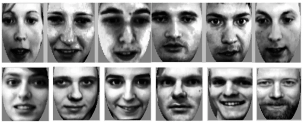
On the results presented on this paper only size normalization of the extracted faces was used. All face images were resized to 130x150 pixels, applying a bi-cubic interpolation. After this stage, it is also developed a position correction algorithm based on detecting the eyes into the face and applying a rotation and resize to align the eyes of all pictures in the same coordinates. The face detection and segmentation tasks presented in this paper was performed based on ‘Face analysis in Polar Frequency Domain’ proposed by Yossi Z. et al. [16]. First it extracts the Fourier-Bessel (FB) coefficients from the images. Next, it computes the Cartesian distance between all the Fourier-Bessel transformation (FBT) representations and re-defines each object by its distance to all other objects. Images were transformed by a FBT up to the 30thBessel order and 6throot with angular resolution of 3˚, thus obtaining to 372 coefficients. These coefficients correspond to a frequency range of up to 30 and 3 cycles/image of angular and radial frequency, respectively. (Figure 1.) Shows 18 still faces extracted from video for user 1 of eNTERFACE2005 dynamics face database [33]. (Figure 2.) Shows the face and eyes detections for different users from two different database, First raw from eNTERFACE 2005 [33] and Second raw from ORL 94 [13] [14]. And (Figure 3.) Shows the face normalization for the same users.

Figure 1. 18 still faces extracted from video for user 1 of eNTERFACE2005 dynamics face database [33].

(4)

Figure 3. Face Normalization for the above users.

Polar Frequency Analysis:

The FB series is useful to describe the radial and angular components in images [16]. FBT analysis starts by converting

the coordinates of a region of interest from Cartesian (x, y) to polar (r, θ). The f (r, θ) function is represented by the two-dimensional FB series, defined as:

, ∑ ∑ , , cos ∑ ∑ , , sin (1)

where Jnis the Bessel function of order n, f (R, θ) = 0 and 0 ≤ r ≤ R. αn, iis the ithroot of the Jnfunction, i.e. the zero crossing value satisfying Jn(αn, i) = 0 is the radial distance to the edge of the image. The orthogonal coefficients An, iand Bn, iare given by:

, _!"#_$_%#_&_',( ) ) , *',(+ , -, "

, . /!

. (2)

if _, 0 1 - 0;

3 ,

,4 #

5+#6'7%# 8*',(9) ) , *',(+

, " , . /!

. 3cos_sin 4 - - (3)

if n > 0.

An alternative method to polar frequency analysis is to represent images by polar Fourier transform descriptors. The polar Fourier transform is a well-known mathematical operation where, after converting the image coordinates from Cartesian to polar, as described above; a conventional Fourier transformation is applied. These descriptors are directly related to radial and angular components, but are not identical to the coefficients extracted by the FBT.

2.2. Face Verification

Feature Extraction:

A. Principal Component Analysis (PCA)

Principal component analysis (PCA) [17] is based on the second-order statistics of the input image, which tries to attain an optimal representation that minimizes the reconstruction error in a least-squares sense. Eigenvectors of the covariance matrix of the face images constitute the eigenfaces. The dimensionality of the face feature space is reduced by selecting only the eigenvectors possessing largest eigenvalues. Once the new face space is constructed, when a test image arrives, it is projected onto this face space to yield the feature vector – the representation coefficients in the constructed face space. The classifier decides for the identity of the individual, according to a similarity score between the test image’s feature vector and the PCA feature vectors of the individuals in the database.

PCA is closely related to the Karhunen-Loève Transform

(KLT) [18, 19], which was derived in the signal processing context as the orthogonal transform with the basis :

;< , … , <>?@ that for any A B C minimize the average D_/

reconstruction error for data points x

E F = GF H ∑I <@F <J. (4) One can show that, under the assumption that the data is zero-mean; the formulations of PCA and KLT are identical. Without loss of generality we will hereafter assume that the data is indeed zero-mean, that is, the mean face FL is always subtracted from the data.

The basis vectors in KLT can be calculated in the following way. Let X be the C M N data matrix whose columns

F , … , FO are observations of a signal embedded in P>; in the context of face recognition, M is the number of available face images and C Q is the number of pixels in an image. The KLT basis : is obtained by solving the eigenvalue problem

R :@_∑:,_where_∑_{is the covariance matrix of the data}

∑ _O∑ F FO @_,₍₅₎

: ;< , … , <S?@ is the eigenvector matrix of ∑, and Λ is the diagonal matrix with eigenvalues T U V U T_> of ∑ on its main diagonal, so that <_W is the eigenvector corresponding to the j-th largest eigenvalue. Then it can be shown that the eigenvalue T is the variance of the data projected on <.

Thus, to perform PCA and extract k principal components of the data, one must project the data onto :_I - the first k

(5)

highest eigenvalues of ∑. This can be seen as a linear projection P> → ℝIthat retains the maximum energy (i.e. variance) of the signal. Another important property of PCA is that it de-correlates the data: the covariance matrix of :_I@Z is always diagonal.

The main properties of PCA are summarized by the following:

F ≈ :I\, :I@:I = ], ^_\ \W`_aW= 0 (6)

Namely, approximate reconstruction, ortho-normality of the basis :_I and de-correlated principal components \ = <@F, respectively. Where PCA is successful in finding the principal manifold where it is less successful, due to clear nonlinearity of the principal manifold.

PCA may be implemented via Singular Value Decomposition (SVD): The SVD of a N × C matrix

Z (N ≥ C) is given by

Z = b c d@_,₍₇₎

Where the N × C matrix U and the C × C matrix V have ortho-normal columns, and the N × C matrix D has the singular values of X on its main diagonal and zero elsewhere. It can be shown thatb = :, so that SVD allows efficient and robust computation of PCA without the need to estimate the data covariance matrix ∑ in Eq. (5). When the number of examples M is much smaller than the dimension N.

B. Linear Discriminate Analysis (LDA)

Linear Discriminate Analysis (LDA) also called Fisher Linear Discriminant (FLD) [20] [21] is an example of a class specific subspace method that finds the optimal linear projection for classification. Rather than finding a projection that maximizes the projected variance as in principal component analysis, FLD determines a projection, \ = Φ_e@F, that maximizes the ratio between the between class scatter and the within-class scatter. Consequently, classification is simplified in the projected space.

Consider a c-class problem, with the between-class scatter matrix given by:

fg= ∑ C (h − h)(h − h)i @ (8)

And the within-class scatter matrix by:

fj = ∑ ∑i kl∈n((FI− h )(FI− h )@ (9)

Where µ is the mean of all samples, h is the mean of class i, and C is the number of samples in class i. The optimal projection Φ_e is the projection matrix which maximizes the ratio of the determinant of the between-class scatter to the determinant of the within-class scatter of the projections,

Φe= 1 o maxsts

u_v_w_st

tsu_v_x_st= ;y y/… yS? (10)

Where zy || = 1, 2, … , Q• is the set of generalized eigenvectors of f_g 1 - f_j, corresponding to the m largest generalized eigenvalues zλ │| = 1, 2, … , Q•. However, the rank of f_g is c-1 or less since it is the sum of c matrices of rank one or less. Thus, the upper bound on m is c-1. To avoid the

singularity, one can apply PCA first to reduce the dimension of the feature space to N-c, and then use FLD to reduce the dimension to c-1. This two-step procedure is used in computing "Fisher Faces".

C. Independent Component Analysis (ICA)

Independent component analysis (ICA) [22] [23] [24] [25] is a statistical method for linear transforming an observed multidimensional random vector X into a random vector Y whose components are stochastically as independent from each other as possible. Several procedures to find such transformations have been recently developed in the signal processing literature relying either on Comon’s [26] information-theoretic approach or Hyvärinen’s maximum negentropy approach [27]. The basic goal of ICA is to find a representation Y = MX (M not necessarily a square matrix) in which the transformed components Yiare the least statistically dependent. ICA leads to meaningful results whenever the probability distribution of X is far from Gaussian and this is the case that we are interested in this paper. For the face recognition task were proposed two different architectures: Architecture I - has statistically independent basis images (ICA I) and Architecture II assumes that the sources are independent coefficients (ICA II). These coefficients give the factorial code representation. The Architecture I provide a more localized representation for faces, while ICA Architecture II, like PCA in a sense, provides a more holistic representation. ICA I produces spatially localized features that are only influenced by small parts of an image, thus isolating particular parts of faces. For this reason ICA I is optimal for recognizing facial actions and suboptimal for recognizing temporal changes in faces or images taken under different conditions. Preprocessing steps of the methods ICA involves a PCA process by vertically centering (for ICA I), and whitened PCA process by horizontally centering (for ICA II). ICA Architecture I include a PCA by vertically centering (PCA I):

‚ƒ= Zƒd@„ … // (11)

Where Z_ƒ is the vertically-centered training image column data matrix. Symbols ˄ and ˅ correspond to largest eigenvalues and eigenvectors of f_@matrix respectively:

f@ = ∑ (F − hO ƒ). (F − hƒ)@, hƒ=_>∑ F>W (12)

In contrast to standard PCA, PCA I removes the mean of each image while standard PCA removes the mean image of all training samples. ICA Architecture II includes a whitened PCA by horizontally centering (PCA II):

‚‡= ‚ˆ. 8_O„ 9 … //

= √NZˆ„ „ … , (13)

Where ‚_ˆ is the projection matrix of standard PCA method:

(6)

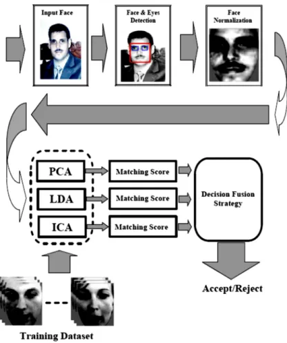
3. Multimodal Biometric Fusion Decision

The process of biometric user authentication can be outlined by the following steps [28]: a) acquisition of raw data, b) extraction of features from these raw data, c) computing a score for the similarity or dissimilarity between these features and a previously given set of reference features and d) classification with respect to the score, using a threshold. The results of the decision processing steps are true

or false (or accept/reject) for verification purposes or the user

identity for identification scenarios.

The fusion of different signals can be performed 1) at the raw data or the feature level, 2) at the score level or 3) at the decision level. These different approaches have advantages and disadvantages. For raw data or feature level fusion, the basis data have to be compatible for all modalities and a common matching algorithm (processing step c) must be used. If these conditions are met, the separate feature vectors of the modalities easily could be concatenated into a single new vector. This level of fusion has the advantage that only one

algorithm for further processing steps is necessary instead of one for each modality. Another advantage of fusing at this early stage of processing is that no information is lost by previous processing steps. The main disadvantage is the demand of compatibility of the different raw data of features. The fusion at score level is performed by computing a similarity or dissimilarity (distance) score for each single modality. For joining of these different scores, normalization should be done. The straightforward and most rigid approach for fusion is the decision level. Here, each biometric modality results in its own decision; in case of a verification scenario this is a set of true's and falsies. From this set a kind of voting (majority decision) or a logical AND or OR decision can be computed. This level of fusion is the least powerful, due to the absence of much information. On the other hand, the advantage of this fusion strategy is the easiness and the guaranteed availability of all single modality decision results. In practice, score level fusion is the best-researched approach, which appears to result in better improvements of recognition accuracy as compared to the other strategies.

Figure 4. Multi-Classifier Face Verification System Framework.

Theoretical Analysis for Decision Level Fusion:

The fusion scheme using these two modalities is denoted by

S. Verification system based only on modality one is denoted by S1, while on modality two by S2 [29]. If Γ is an algorithm, then the task is to find which acts on independent sources so that the output is maximized. It can be written as:

(7)

Ž •(•) = ‚(y‘ |y ) = ) ’(Z|y_"_% )-Z = 1 − ) ’(Z|y_"_“ )-Z, (16)

Ž••(•) = ‚(y‘ |y ) = ) ’(Z|y )_"_“ -Z (17)

Where w1 denotes the genuine user while w0 denotes by the

imposter one. R0 and R1 are two exclusive sets in real axis.

Both FAR and FRR are desirable to be as low as possible in authentication system. For any biometrics authentication system, whatever classifier takes, there exists a great risk of error. From the viewpoint of Bayesian decision theory, this is represented by the following equations for a two class problem,

^(•) = ”, × Ž••(•) + ”• × Ž •(•), (18)

^ (• ) = ”, × Ž•• (• ) + ”• × Ž • (• ), – | = 1, . . , C (19) Where, N is the total modalities number, Cr denotes the loss

function pertinent to the false rejection, and Ca denotes the

loss function for the false acceptance. For simplicity, it assume that ”_•= ”_• 1 - ”_,= ”_,.

Decision level fusion:

The integrated system is denoted by Ψ. The outputs by individual systems Ψ1 and Ψ2, are called scores, which stand

for the probability of claimant to be a genuine or an imposter. For any fusion strategies, an error is expressed as (18) and (19). If it assumes that ^ (• ) ≤ ^_/(•_/) ≤. . ≤ ^_>(•_>), then it is easily known it is sufficient to prove that ^(•) ≤ ^ (• ). For a two-modality and Bayesian rule Fusion:

Decide w0, if (X1, X2) ∈ • (20)

Decide w1, otherwise

Where • = z (Z , Z_/)|”_,’(Z , Z_/|y ) ≥ ”_•’(Z , Z_/|y ) •.

Since Ψ1 and Ψ2 are independent, it have:

’(Z , Z/|y ) = ’ (Z |y )’/(Z/|y ), (21)

&

’(Z , Z/|y ) = ’ (Z |y )’/(Z/|y ), (22) Then:

Ž •(•) = 1 − — ’(Z , Z/|y )-Z -Z/

"“

= 1 − ) ’ (Z |y_"_“ )-Z ) ’_"_“ /(Z/|y )-Z/ (23)

= 1 − 1 − Ž • (• ) 1 − Ž •/_(•_/_{) .}

&

Ž••(•) = 1 − — ’(Z , Z/|y )-Z -Z/

"“

= 1 − ) ’ (Z |y )-Z_"_“ ) ’_"_“ /(Z/|y )-Z/ (24)

= Ž•• (• )Ž••/_(•_/_).

From the Equations (14) & (15) it can be obviously seen that:

Ž •(•) = Ž • (• ) and Ž •(•) = Ž •/(•_/). Thus the

two combined modalities cannot improve the false acceptance rate by the Bayesian decision rule. Otherwise Ž••(•) =

Ž•• (• ) and Ž••(•) = Ž••/(•_/). Hence the false rejection

rate of the combined system is reduced compared to individual sub-classifiers.

Maximum Likelihood Parameter Estimation:

Given a set of observation data in a matrix X and a set of observation parameters the ML parameter estimation aims at maximizing the likelihood D( )or log likelihood of the observation data Z = zZ , … , Z •

‹ = 1 o max_. D( ). (25)

Assuming that it has independent, identically distributed data, it can write the above equations as:

D( ) = ’(Z| ) = ’(Z , … , Z | ) = ∏ ’(Z | ). (26)

The maximum for this function can be find by taking the derivative and set it equal to zero, assuming an analytical function.

™

™.D( ) = 0. (27)

The incomplete-data log-likelihood of the data for the mixture model is given by:

D( ) = š–o(Z| ) =∑ š–o F |> ₍₂₈₎

Which is difficult to optimize because it contains the log of the sum. If it considers X as incomplete, however, and posits the existence of unobserved data items › z\ •> whose values inform us which component density generated each data item, the likelihood expression is significantly simplified. That is, it assume that \ m z1. . œ• for each i, and \ = Aif the i-th sample was generated by the k-th mixture component. If it knows the values of Y, it obtains the complete-data log-likelihood, given by:

D( , ›) = log ’(Z, ›| ) (29)

=∑> log ’(F , \ | )₍₃₀₎ =∑> log ’(\ | )’(F |\ , ) ₍₃₁₎ = ∑> log ’Ÿ(+ log o F thŸ(,∑Ÿ( (32)

Which, given a particular form of the component densities, can be optimized using a variety of techniques [30].

4. Experiments and Results Discussion

(8)

[33]:

ORL 94 [13, 14] Olivetti Research Laboratories (ORL 94) database of faces provides 10 sample images of each of 40 subjects (in PGM files format) in which four subjects are females and thirty six are males. The primary age grouping of the individuals captured seems to range from the late 20’s to the mid 30’s. Clearly there is an under representation of young and old people. The different images for each subject provide variation in views of the individual such as lighting, facial features (such as glasses), and slight changes in head orientation. It chose to use this face database because it seemed to be a standard set of test images used in much of the literature we encountered dealing with face recognition.

INDIAN FACES DATABASE 2002 (IFD2002) [15] this database contains human face images of 60 subjects (640x480 JPEG files format) with eleven different poses for each individual in which thirty nine are males and twenty two are females, the images were captured in February, 2002 in the campus of Indian Institute of Technology Kanpur. All the images have a bright homogeneous background and the subjects are in an upright, frontal position. For each individual, it have included the following pose for the face: looking front, looking left, looking right, looking up, and looking up towards left, and looking up towards right, looking down. In addition to the variation in pose, images with four emotions - neutral, smile, laughter, sad/disgust - are also included for every individual.

eNTERFACE 2005 Still Faces Databases [33] this database extracted from video, which is encoded in raw UYVY. AVI 640 x 480, 15.00 fps with uncompressed 16bit PCM audio; mono, 32000 Hz little endian. Uncompressed PNG files are extracted from the video files for feeding the face detection algorithms. The capturing devices for recording the video and audio data were: Allied Vision Technologies AVT marlin MF-046C 10 bit ADC, 1/2” (8mm) Progressive scan SONY IT CCD; and Shure SM58 microphone. Frequency response 50 Hz to 15000 Hz. Unidirectional (Cardiod) dynamic vocal microphones. Thirty subjects were used for the experiments in which twenty-six are males and four are females. For each subject, the database obtained from eNTERFACE 2005 [33]. For Each user of still face experts, seventy-two still face images from a subject were randomly selected for training, and the other forty-eight samples were used for the subsequent validation and testing. Three sessions of the still face database, were used separately. Session one was used for training the still face experts. To find the performance, Sessions two and three were used for obtaining expert opinions of known impostor and true claims.

For both Independent Component Analysis Architectures I and II, it employed two novel processing design algorithmic analyses and generates scores using three different similarity measures algorithms (Cosine Similarity, City Block and Square Euclidean Distances Similarity) [31, 32], and the performance of the analysis design for the likelihood ratio are based on EER (Equal Error Rate) of the ROC (Receptive Operation Characteristics) plotting evaluation.

For algorithmic processing design one (One Image Processing): at the preprocessing phase each representation of

the databases training and testing is normalized (divided on the square root of its power); at the fundamental processing phase, it computing the scores (Similarity Distances Measures) of the testing normalized representation with normalized training representation; for ORL94 Face Databases in which 60% of the data size are used for training and 40% of the data size are used for testing: that gives 4x6=24 Similarity Distances for each user; Thus 40x (4x6)=960 target scores. For IFD2002 60x (4x6)=1440 target scores. for eNTERFACE 2005 still faces databases [33]. In which 60% of the data size are used for training and 40% of the data size are used for validation and testing: that gives 48x72=3456 Similarity Distances for each user; Thus 30x (48x72)=103680 target scores. Thus the target scores, noted (tscores) are built using Normal Law of probability ɴ (tscores, tm, ts2) of the mean tm and standard deviation ts. Then, computing the scores of Distances Similarity Measures between the normalized representations of the test users with the normalized representation of the training users; Thus, it gives 4x6x39=936 scores for each user; hence the total non-target scores are 40x (4x6x39)=37440 for ORL94; and 60x (4x6x59)=84960 for IFD2002. Thus, it gives 48x72x29=100224 scores for each user; hence the total non-target scores are 30x (48x72x29)= 3006720. These non-target scores, noted (nscores), are built using Normal Law of probability ɴ (nscores, nm, ns2) of the mean nm and standard deviation ns.

Then; computing the Logarithmic Ration of the Likelihood for tscores and nscores with:

LR¢£¤¥¦§£= log N(tscores, tm, ts/)

− log N(tscores, nm, ns/₎

&

LR¬£¤¥¦§£= log N(nscores, tm, ts/)

− log N(nscores, nm, ns/₎

Then; Evaluated the ROC and the EER.

(9)

probability ɴ (mtscores, mtm, mts2) of the mean mtm and standard deviation mts. Then, computing the scores of Distances Similarity Measures between the normalized representations of the test users with the normalized representation of the training users; Thus, it gives 4x6x39=936 scores for each user for ORL94, 4x6x59=1416 for IFD2002 and 48x72x29=100224 scores for eNTERFACE2005 for each user; for each user it compute the mean of its 936, 1416 and 100224 scores respectively. And computed the non-target scores respectively for ORL94, IFD2002 and eNTERFACE2005. These non-target scores, noted (mnscores), are built using Normal Law of probability ɴ (mnscores, mnm, mns2) of the mean mnm and standard deviation mns.

Then; computing the Logarithmic Ration of the Likelihood for tscores and nscores with:

LR¢£¤¥¦§£ log N mtscores, tm, mts/

H log N mtscores, mnm, mns/

&

LR¬£¤¥¦§£ log N mnscores, mtm, mts/

H log N mnscores, mnm, mns/

Then; Evaluated the ROC and the EER.

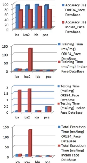
The Figure 5., Show the Pattern Recognition Analysis Performance studies [The Systems Used for the simulation studies are: i5 Intel Core Processor (2.66Ghz, 3MB L3 cache); 8 GB DDR3 Memory and Windows 8 Operating Systems & MATLAB 2014a Programming Tools]; and the Figure 6., show the Verification Analysis Studies Based Olivetti Research Laboratories (ORL 94) Face databases for Independent Components Analysis Classifier Fusion of Likelihood Ratio; the Figure 7., show the Verification Analysis Studies Based Indian Face databases for Independent Components Analysis Classifier Fusion of Likelihood Ratio;

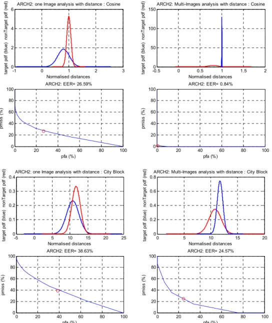
And the Figure 8., show the Verification Analysis Studies Based eNTERFACE2005 Dynamic Face databases for Independent Components Analysis Classifier Fusion of Likelihood Ratio.

(10)

-2 -1 0 1 2 3 0 0.5 1 1.5 2 Normalised distances ta rg e t p d f (r e d ) n o n T a rg e t p d f (b lu e

) _{ARCH1: one Image analysis with distance : Cosine}

0 20 40 60 80 100

0 20 40 60 80 100 pfa (%) p m is s ( % )

ARCH1: EER= 12.38%

-0.50 0 0.5 1 1.5

20 40 60 Normalised distances ta rg e t p d f (b lu e ) n o n T a rg e t p d f (r e d )

ARCH1: Multi-Images analysis with distance : Cosine

0 20 40 60 80 100

0 20 40 60 80 100 pfa (%) p m is s ( % )

ARCH1: EER= 0%

-10 0 10 20 30

0 0.1 0.2 0.3 0.4 Normalised distances ta rg e t p d f (r e d ) n o n T a rg e t p d f (b lu e

) _{ARCH1: one Image analysis with distance : City Block}

0 20 40 60 80 100

0 20 40 60 80 100 pfa (%) p m is s ( % )

ARCH1: EER= 12.57%

-5 0 5 10 15 20

0 1 2 3 Normalised distances ta rg e t p d f (b lu e ) n o n T a rg e t p d f (r e d

) ARCH1: Multi-Images analysis with distance : City Block

0 20 40 60 80 100

0 20 40 60 80 100 pfa (%) p m is s ( % )

ARCH1: EER= 0%

-0.50 0 0.5 1 1.5 2 2.5 3

2 4 6 8 Normalised distances ta rg e t p d f (b lu e ) n o n Ta rg e t p d f (r e d )

ARCH2: one Image analysis with distance : Euclidean

0 20 40 60 80 100

0 20 40 60 80 100 pfa (%) p m is s ( % )

ARCH2: EER= 24.96%

0.8 1 1.2 1.4 1.6 1.8

0 100 200 300 400 Normalised distances ta rg e t p d f (b lu e ) n o n Ta rg e t p d f (r e d )

ARCH2: Multi-Images analysis with distance : Euclidean

0 20 40 60 80 100

0 20 40 60 80 100 pfa (%) p m is s ( % )

(11)

Figure 6. Verification Analysis Studies Based Olivetti Research Laboratories (ORL 94) Face databases for Independent Components Analysis Classifier Fusion of Likelihood Ratio.

-1 0 1 2 3

0 2 4 6 Normalised distances ta rg e t p d f (b lu e ) n o n T a rg e t p d f (r e d )

ARCH2: one Image analysis with distance : Cosine

0 20 40 60 80 100

0 20 40 60 80 100 pfa (%) p m is s ( % )

ARCH2: EER= 24.19%

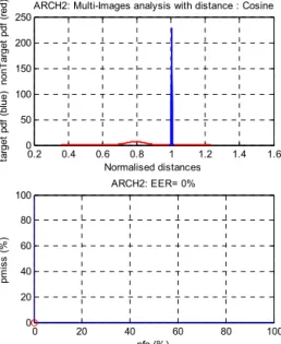
0.2 0.4 0.6 0.8 1 1.2 1.4 1.6 0 50 100 150 200 250 Normalised distances ta rg e t p d f (b lu e ) n o n T a rg e t p d f (r e d )

0 20 40 60 80 100

0 20 40 60 80 100 pfa (%) p m is s ( % )

ARCH2: EER= 0%

-5 0 5 10 15 20 25

0 0.1 0.2 0.3 0.4 Normalised distances ta rg e t p d f (b lu e ) n o n T a rg e t p d f (r e d

) _{ARCH2: one Image analysis with distance : City Block}

0 20 40 60 80 100

0 20 40 60 80 100 pfa (%) p m is s ( % )

ARCH2: EER= 40.98%

0 5 10 15 20

0 0.2 0.4 0.6 0.8 1 Normalised distances ta rg e t p d f (b lu e ) n o n T a rg e t p d f (r e d

) _{ARCH2: Multi-Images analysis with distance : City Block}

0 20 40 60 80 100

0 20 40 60 80 100 pfa (%) p m is s ( % )

ARCH2: EER= 22.5%

-2 -1 0 1 2 3 4

0 0.5 1 1.5 2 2.5 Normalised distances ta rg e t p d f (r e d ) n o n Ta rg e t p d f (b lu e )

0 20 40 60 80 100

0 20 40 60 80 100 pfa (%) p m is s ( % )

ARCH1: EER= 15.78%

-0.50 0 0.5 1 1.5 2 2.5

5 10 15 20 Normalised distances ta rg e t p d f (b lu e ) n o n Ta rg e t p d f (r e d )

0 20 40 60 80 100

0 20 40 60 80 100 pfa (%) p m is s ( % )

(12)

-2 -1 0 1 2 3 0 0.5 1 1.5 2 Normalised distances ta rg e t p d f (r e d ) n o n T a rg e t p d f (b lu e )

0 20 40 60 80 100

0 20 40 60 80 100 pfa (%) p m is s ( % )

ARCH1: EER= 15.78%

-1 -0.5 0 0.5 1 1.5 2

0 20 40 60 80 100

0 20 40 60 80 100 pfa (%) p m is s ( % )

ARCH1: EER= 0%

-20 -10 0 10 20 30

0 0.05 0.1 0.15 0.2 Normalised distances ta rg e t p d f (r e d ) n o n T a rg e t p d f (b lu e )

ARCH1: one Image analysis with distance : City Block

0 20 40 60 80 100

0 20 40 60 80 100 pfa (%) p m is s ( % )

ARCH1: EER= 14.44%

-5 0 5 10 15 20 25

0 0.5 1 1.5 2 Normalised distances ta rg e t p d f (b lu e ) n o n T a rg e t p d f (r e d )

ARCH1: Multi-Images analysis with distance : City Block

0 20 40 60 80 100

0 20 40 60 80 100 pfa (%) p m is s ( % )

ARCH1: EER= 0%

-0.50 0 0.5 1 1.5 2 2.5 3

0 20 40 60 80 100

0 20 40 60 80 100 pfa (%) p m is s ( % )

ARCH2: EER= 27.5%

0 0.5 1 1.5 2 2.5

0 50 100 150 200 Normalised distances ta rg e t p d f (b lu e ) n o n T a rg e t p d f (r e d )

0 20 40 60 80 100

0 20 40 60 80 100 pfa (%) p m is s ( % )

(13)

Figure 7. Verification Analysis Studies Based Indian Face databases for Independent Components Analysis Classifier Fusion of Likelihood Ratio.

-1 0 1 2 3

0 2 4 6 Normalised distances ta rg e t p df ( b lu e ) n o nT a rge t p d f (r e d )

0 20 40 60 80 100

0 20 40 60 80 100 pfa (%) p m is s ( % )

ARCH2: EER= 26.59%

-0.50 0 0.5 1 1.5 2

50 100 150 Normalised distances ta rg e t p df ( b lu e ) n o nT a rge t p d f (r e d )

0 20 40 60 80 100

0 20 40 60 80 100 pfa (%) p m is s ( % )

ARCH2: EER= 0.84%

-5 0 5 10 15 20 25

0 0.1 0.2 0.3 0.4 Normalised distances ta rg e t p d f (b lu e ) n o n T a rg e t p d f (r e d )

ARCH2: one Image analysis with distance : City Block

0 20 40 60 80 100

0 20 40 60 80 100 pfa (%) p m is s ( % )

ARCH2: EER= 38.63%

0 5 10 15 20

0 0.2 0.4 0.6 0.8 Normalised distances ta rg e t p d f (b lu e ) n o n T a rg e t p d f (r e d )

ARCH2: Multi-Images analysis with distance : City Block

0 20 40 60 80 100

0 20 40 60 80 100 pfa (%) p m is s ( % )

ARCH2: EER= 24.57%

-2 -1 0 1 2 3

0 1 2 3 Normalised distances ta rg e t p d f (r e d ) n o n T a rg e t p d f (b lu e

) ARCH1: Single User Images analysis _{with distance : Euclidean}

0 20 40 60 80 100

0 20 40 60 80 100 pfa (%) p m is s ( % )

ARCH1: EER= 0.61%

-1 -0.5 0 0.5 1 1.5

0 10 20 30 40 50 Normalised distances ta rg e t p d f (b lu e ) n o n T a rg e t p d f (r e d

) ARCH1: Multi-Users Images analysis _{with distance : Euclidean}

0 20 40 60 80 100

0 20 40 60 80 100 pfa (%) p m is s ( % )

(14)

-1 0 1 2 3 0 1 2 3 4 5 Normalised distances ta rg e t p d f (r e d ) n o n T a rg e t p d f (b lu e

) ARCH1: Single User Images analysis _{with distance : Cosine}

0 20 40 60 80 100

0 20 40 60 80 100 pfa (%) p m is s ( % )

ARCH1: EER= 1.21%

-1 -0.5 0 0.5 1 1.5

) ARCH1: Multi-Users Images analysis _{with distance : Cosine}

0 20 40 60 80 100

0 20 40 60 80 100 pfa (%) p m is s ( % )

ARCH1: EER= 0%

-10 0 10 20 30

0 0.1 0.2 0.3 0.4 Normalised distances ta rg e t p d f (r e d ) n o n T a rg e t p d f (b lu e

) ARCH1: Single User Images analysis _{with distance : City Block}

0 20 40 60 80 100

0 20 40 60 80 100 pfa (%) p m is s ( % )

ARCH1: EER= 1.41%

-10 -5 0 5 10 15

0 0.5 1 1.5 2 Normalised distances ta rg e t p d f (b lu e ) n o n T a rg e t p d f (r e d

) ARCH1: Multi-Users Images analysis _{with distance : City Block}

0 20 40 60 80 100

0 20 40 60 80 100 pfa (%) p m is s ( % )

ARCH1: EER= 0%

-2 0 2 4 6

) ARCH2: Single User Images analysis _{with distance : Euclidean}

0 20 40 60 80 100

0 20 40 60 80 100 pfa (%) p m is s ( % )

ARCH2: EER= 16.91%

0.5 1 1.5 2

) ARCH2: Multi-Users Images analysis _{with distance : Euclidean}

0 20 40 60 80 100

0 20 40 60 80 100 pfa (%) p m is s ( % )

(15)

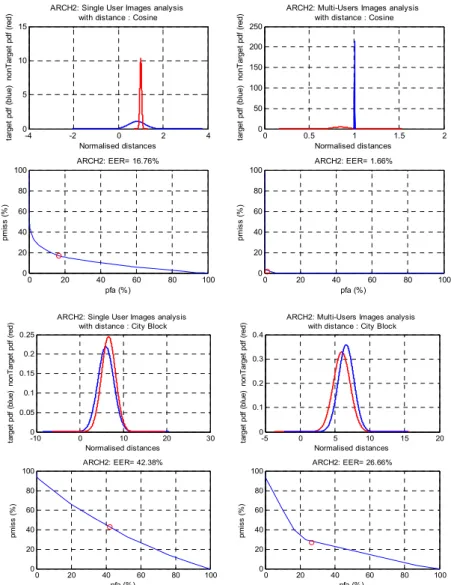
Figure 8. Verification Analysis Studies Based eNTERFACE2005 Dynamics Face databases for Independent Components Analysis Classifier Fusion of Likelihood Ratio.

5. Conclusions

The paper has presented a human authentication method of Biometric face based Independent Component Analysis Architectures I and II; single biometric authentication has the fundamental problems of high FAR and FRR. It has presented a framework for novel fusion strategy within the scores at the score level. The likelihood ratio based fusion rule within the scores of the classifier achieves a significant recognition rates. As a result presented an EER=0.61%. And EER=0.00%. Respectively for Algorithmic Processing design One and Two of algorithmic design Based ICA ARCH I fusion of Likelihood Ratio within scores are achieved based Euclidean Measures Similarity. Thus, Based on the experimental results, it has shown that EER can be reduced down significantly.

References

[1] S. Gleni and P. Petratos, DNA Smart Card for Financial Transactions, The ACM Student Magazine 2004, http://www.acm.org.

[2] G. Chetty and M. Wagner, Audio-Visual Multimodal Fusion for Biometric Person Authentication and Liveness Verification,

Australian Computer Society, Inc. This paper appeared at the NICTA-HCSNet Multimodal UserInteraction Workshop (MMUI2005), Sydney, Australia.

[3] N. Poh and S. Bengio, Database, Protocol and Tools for Evaluating Score-Level Fusion Algorithms in Biometric Authentication, IDIAP RR 04-44, August 2004, a IDIAP, CP 592, 1920 Martigny, Switzerland.

[4] S. Srisuk, M. Petrou, W. Kurutach and A. Kadyrov, Face Authentication using the Trace Transform, Proceedings of the 2003 IEEE Computer Society Conference on Computer Vision and Pattern Recognition (CVPR’03).

[5] S. Ben-Yacoub, Y. Abdeljaoued, and E. Mayoraz, Fusion of Face and Speech Data for Person Identity Verification, IEEE TRANSACTIONS ON NEURAL NETWORKS, VOL. 10, NO. 5, SEPTEMBER 1999.

[6] J. Kittler, M. Hatef, Robert P. W. Duin, and J. Matas, On Combining Classifiers, IEEE TRANSACTIONS ON PATTERN ANALYSIS AND MACHINE INTELLIGENCE, VOL. 20, NO. 3, MARCH 1998.

-4 -2 0 2 4

) ARCH2: Single User Images analysis _{with distance : Cosine}

0 20 40 60 80 100

0 20 40 60 80 100 pfa (%) p m is s ( % )

ARCH2: EER= 16.76%

0 0.5 1 1.5 2

0 50 100 150 200 250 Normalised distances ta rg e t p d f (b lu e ) n o n T a rg e t p d f (r e d

) ARCH2: Multi-Users Images analysis _{with distance : Cosine}

0 20 40 60 80 100

0 20 40 60 80 100 pfa (%) p m is s ( % )

ARCH2: EER= 1.66%

-10 0 10 20 30

0 0.05 0.1 0.15 0.2 0.25 Normalised distances ta rg e t p d f (b lu e ) n o n T a rg e t p d f (r e d

) ARCH2: Single User Images analysis _{with distance : City Block}

0 20 40 60 80 100

0 20 40 60 80 100 pfa (%) p m is s ( % )

ARCH2: EER= 42.38%

-5 0 5 10 15 20

0 0.1 0.2 0.3 0.4 Normalised distances ta rg e t p d f (b lu e ) n o n T a rg e t p d f (r e d

) ARCH2: Multi-Users Images analysis _{with distance : City Block}

0 20 40 60 80 100

0 20 40 60 80 100 pfa (%) p m is s ( % )

(16)

[7] B. Batagelj and F. Solina, Face Recognition in Different Subspaces: A Comparative Study, University of Ljubljana, Faculty of Computer and Information Science, Trzaska 25, SI-1000 Ljubljana, Slovenia.

[8] X. Lu, Y. Wang and A.K. Jain, Combining Classifiers for Face Recognition, Proc. ICME 2003 (IEEE International Conference on Multimedia & Expo), Baltimore, MD, July 6-9, 2003, pp. 13-16.

[9] Brian C. Becker and Enrique G. Ortiz , Evaluation of Face Recognition Techniques for Application to Face-book, 8th IEEE International Conference on Automatic Face & Gesture Recognition, 2008 (FG '08)., December, 2009.

[10] K. Delac, M. Grgic, S. Grgic, Independent Comparative study of PCA, ICA and LDA on the FERET Data set, Proc. of the 4th International Symposium on Image and Signal Processing and Analysis, pp 289-294, 2005.

[11] K. Veeramachaneni, L. Osadciw, A. Ross and N. Srinivas, Decision-level Fusion Strategies for Correlated Biometric Classifiers, Proc. of IEEE Computer Society Workshop on Biometrics at the Computer Vision and Pattern Recogniton (CVPR) conference, (Anchorage, USA), June 2008.

[12] H. K. Ekenel and B. Sankur, Multiresolution face recognition, Electrical and Electronic Engineering Department, Bogazici University, Bebek, I˙stanbul, Turkey-Received 30 January 2004; accepted 17 September 2004. Elsevier B. V.

[13] Olivetti Research Laboratories face database, ORL 1994, http://www.cl.cam.ac.uk/research/dtg/attarchive/facedatabase. html.

[14] F. Samaria and A. Harter, Parameterization of a stochastic model for human face identification, 2nd IEEE Workshop on Applications of Computer Vision, Sarasota (Florida), December 1994.

[15] Vidit Jain and Amitabha Mukherjee. The Indian Face Database 2002.

http://vis-www.cs.umass.edu/~vidit/IndianFaceDatabase/. [16] Y. Zana, Roberto M. Cesar-Jr, Rogerio S. Feris, and Matthew

Turk, Face Verification in Polar Frequency Domain: A Biologically Motivated Approach, ISVC 2005, LNCS 3804, pp. 183–190, 2005. C Springer-Verlag Berlin Heidelberg 2005 [17] M. Turk and A. Pentland, Eigenfaces for Recognition, Journal

of Cognitive Neuroscience, vol. 3, no. 1, pp. 71-86, 1991. [18] G. Shakhnarovich and B. Moghaddam, Face Recognition in

Subspaces, TR2004-041 May 2004. Electric Research Laboratories, Inc., 2004 - 201 Broadway, Cambridge, Massachusetts 02139.

[19] M. M. Loève. Probability Theory, Van Nostrand, Princeton, 1955. [20] V. Belhumeur, J. Hespanha, and D. Kriegman, Eigenfaces vs. Fisherfaces: Recognition using class specific linear projection. IEEE Transactions on Pattern Analysis and Machine Intelligence, 19 (7): 711-720, July 1997.

[21] S. Bn-Yacoub, Y. Abdljaoued and E. Mayoraz, FUSION OF FACE AND SPEECH DATA FOR PERSON IDENTITY VERIFICATION, IDIAP-RR 99-2003.

[22] A. Hyvärinen and E. Oja, Independent Component Analysis: Algorithms and Applications, Neural Networks Research Centre Helsinki University of Technology, P. O. Box 5400, FIN-02015 HUT, Finland Neural Networks, 13 (4-5): 411-430, 2000.

[23] W. Lu and Jagath C. Rajapakse, Constrained Independent Component Analysis, School of Computer Engineering – Nanyang Technological University, Singapore 639798. [24] S. Vaseghi and H. Jetelova, Principal and independent

component analysis in image processing, in Proceedings of the 14th ACM International Conference on Mobile Computing and Networking (MOBICOM ’06) , pp. 1–5, San Francisco, Calif, USA, September 2006.

[25] M. S. Bartlett, H. M. Lades, T. J. Sejnowski, Independent component representations for face recognition, Conference on Human Vision and Electronic Imaging III, San Jose, California, 1998.

[26] P. Comon, Independent component analysis, a new concept, Signal Processing36, 287–314 (1994).

[27] A. Hyvärinen, Independent component analysis by minimization of mutual information, Proc. IEEE Int. Conf. on Acoustics, Speech and Signal Processing (ICASSP’97), 3917–3920 (1997). [28] K. Veeramachaneni, L. A. Osadciw, and P. K. Varshney, An Adaptive Multimodal Biometric Management Algorithm, IEEE TRANSACTIONS ON SYSTEMS, MAN, AND CYBERNETICS-PART C: APPLICATIONS AND REVIEWS, VOL. 35, NO. 3, AUGUST 2005.

[29] D. Huang, H. Leung and Winston Li, Fusion of Dependent and Independent Biometric Information Sources, Department of Electrical & Computer Engineering - University of Calgary, 2500 University Dr NW Calgary, AB T2N 1N4.

[30] P. Minh Tri, On estimating the parameters of Gaussian mixtures using EM, School of Computer Engineering, Nanyang Technological University.

[31] Distance Measures Overview,

https://docs.tibco.com/pub/spotfire/5.5.0-march-2013/UsersG uide/hc/hc_distance_measures_overview.htm

[32] Distance Measures,

http://www.umass.edu/landeco/teaching/multivariate/readings/ McCune.and.Grace. 2002.chapter6.pdf.

[33] Yannis S., Yannis P., Felipe C., Pedro L., Francois S., Sascha S., Rolando B., Federico M., and Athanasios V., GMM-Based Multimodal Biometric Verification, eNTERFACE 2005 The summer Workshop on Multimodal Interfaces July 18th – August 12th, Facultè Polytechnique de Mons, Belgium.