Explicit computations with modular
Galois representations
Proefschrift
ter verkrijging van
de graad van Doctor aan de Universiteit Leiden,
op gezag van Rector Magnificus prof. mr. P. F. van der Heijden,
volgens besluit van het College voor Promoties
te verdedigen op maandag 15 december 2008
klokke 13.45 uur
door
Johannes Gerardus Bosman
Promotor: prof. dr. S. J. Edixhoven (Universiteit Leiden)
Referent: prof. dr. W. A. Stein (University of Washington)
Overige leden: prof. dr. J.-M. Couveignes (Universit´e de Toulouse 2) prof. dr. J. Kl¨uners (Heinrich-Heine-Universit¨at D¨usseldorf) prof. dr. H. W. Lenstra, Jr. (Universiteit Leiden)
FOR
M
ATHEMATICS
Johan Bosman, Leiden 2008
Contents
Preface vii
1 Preliminaries 1
1.1 Modular forms . . . 1
1.1.1 Definitions . . . 1
1.1.2 Example: modular forms of level one . . . 4
1.1.3 Eisenstein series of arbitrary levels . . . 7
1.1.4 Diamond and Hecke operators . . . 10
1.1.5 Eigenforms . . . 14
1.1.6 Anti-holomorphic cusp forms . . . 16
1.1.7 Atkin-Lehner operators . . . 16
1.2 Modular curves . . . 17
1.2.1 Modular curves overC . . . 18
1.2.2 Modular curves as fine moduli spaces . . . 19
1.2.3 Moduli interpretation at the cusps . . . 21
1.2.4 Katz modular forms . . . 24
1.2.5 Diamond and Hecke operators . . . 27
1.3 Galois representations associated to newforms . . . 27
1.3.1 Basic definitions . . . 28
1.3.2 Galois representations . . . 29
1.3.3 `-Adic representations associated to newforms . . . 30
1.3.4 Mod`representations associated to newforms . . . 32
1.3.5 Examples . . . 34
1.4 Serre’s conjecture . . . 35
1.4.1 Some local Galois theory . . . 35
1.4.2 The level . . . 38
1.4.3 The weight . . . 39
1.4.4 The conjecture . . . 41
2 Computations with modular forms 43 2.1 Modular symbols . . . 43
2.1.1 Definitions . . . 43
2.1.2 Properties . . . 45
2.1.3 Hecke operators . . . 46
2.1.4 Manin symbols . . . 47
2.2 Basic numerical evaluations . . . 49
2.2.1 Period integrals: the direct method . . . 50
2.2.2 Period integrals: the twisted method . . . 51
2.2.3 Computation ofq-expansions at various cusps . . . 52
2.2.4 Numerical evaluation of cusp forms . . . 55
2.2.5 Numerical evaluation of integrals of cusp forms . . . 56
2.3 Computation of modular Galois representations . . . 58
2.3.1 Computing representations forτ(p)mod` . . . 58
2.3.2 Computingτ(p)mod`fromP` . . . 62
2.3.3 Explicit numerical computations . . . 62
3 A polynomial with Galois groupSL2(F16) 69 3.1 Introduction . . . 69
3.1.1 Further remarks . . . 70
3.2 Computation of the polynomial . . . 71
3.3 Verification of the Galois group . . . 72
3.4 DoesPindeed defineρf? . . . 74
3.4.1 Verification of the level . . . 75
3.4.2 Verification of the weight . . . 76
3.4.3 Verification of the form f . . . 77
3.5 MAGMAcode used for computations . . . 78
4 Some polynomials for level one forms 79 4.1 Introduction . . . 79
4.1.1 Notational conventions . . . 79
4.1.2 Statement of results . . . 80
4.2 Galois representations . . . 81
4.2.1 Liftings of projective representations . . . 81
4.2.2 Serre invariants and Serre’s conjecture . . . 82
4.2.3 Weights and discriminants . . . 82
4.3 Proof of the theorem . . . 84
4.4 Proof of the corollary . . . 86
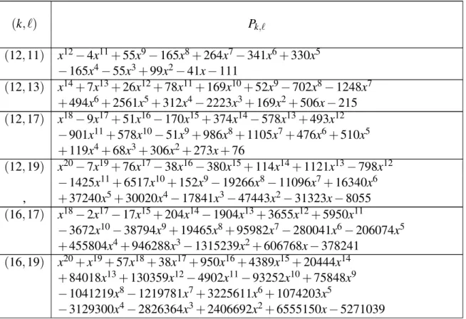
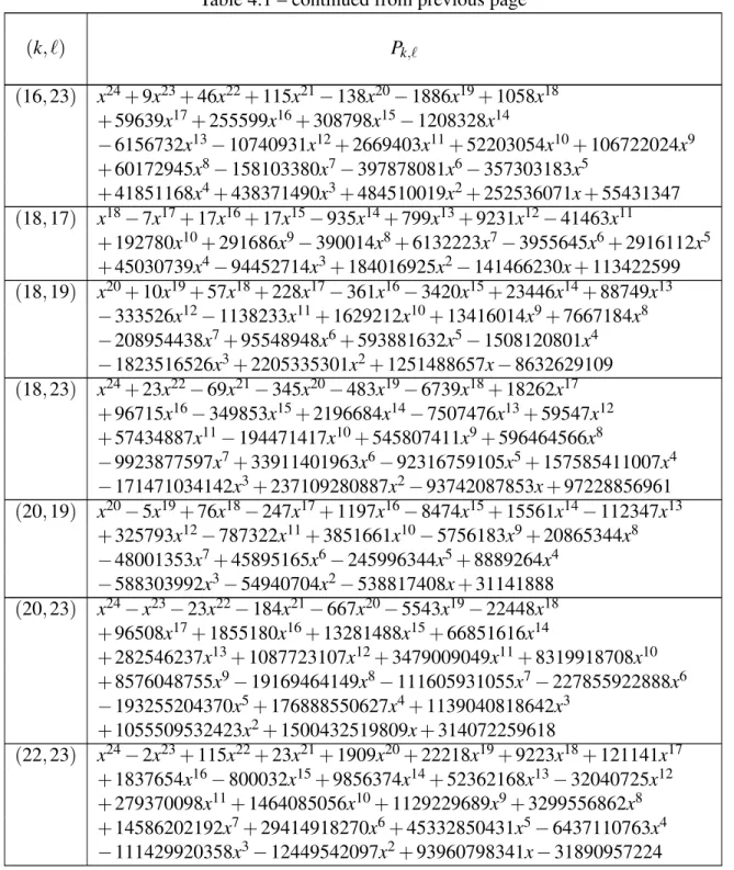
4.5 The table of polynomials . . . 87
Bibliography 89
Samenvatting 95
Curriculum vitae 101
Preface
The area of modular forms is one of the many junctions in mathematics where several dis-ciplines come together. Among these disdis-ciplines are complex analysis, number theory, al-gebraic geometry and representation theory, but certainly this list is far from complete. In fact, the phrase ‘modular form’ has no precise meaning since modular forms come in many types and shapes. In this thesis, we shall be working with classical modular forms of integral weight, which are known to be deeply linked with two-dimensional representations of the absolute Galois group of the field of rational numbers.
In the past decades an astonishing amount of research has been performed on the deep the-oreticalaspects of these modular Galois representations. The most well-known result that came out of this is the proof of Fermat’s Last Theorem by Andrew Wiles. This theorem states that for any integern>2, the equationxn+yn=zn has no solutions in positive integersx, yandz. The fact that at first sight this theorem seems to have nothing to do with modular forms at all witnesses the depth as well as the broad applicability of the theory of modu-lar Galois representations. Another big result has been achieved, namely a proof of Serre’s conjecture by Chandrashekhar Khare, Jean-Pierre Wintenberger and Mark Kisin. Serre’s conjecture states that every continuous two-dimensional odd irreducible residual representa-tion of Gal(Q/Q)comes from a modular form. This can be seen as a vast generalisation of Wiles’s result and in fact the proof also uses Wiles’s ideas.
On the other hand, research on thecomputationalaspects of modular Galois representations is still in its early childhood. At the moment of writing this thesis there is very little literature on this subject, though more and more people are starting to perform active research in this field. This thesis is part of a project, led by Bas Edixhoven, that focuses on the computations of Galois representations associated to modular forms. The project has a theoretical side, proving computability and giving solid runtime analyses, and an explicit side, performing actual computations. The main contributors to the theoretical part of the project are, at this moment of writing, Bas Edixhoven, Jean-Marc Couveignes, Robin de Jong and Franz Merkl. A preprint version of their work, which will eventually be published as a volume of the An-nals of Mathematics Studies, is available [28]. As the title of this thesis already suggests, we will be dealing with the explicit side of the project. In the explicit calculations we will make some guesses and base ourselves on unproven heuristics. However, we will use Serre’s conjecture to prove the correctness of our results afterwards.
The thesis consists of four chapters. In Chapter 1 we will recall the relevant parts of the theory of modular forms and Galois representations. It is aimed at a reader who hasn’t studied this subject before but who wants to be able to read the rest of the thesis as well. Chapter 2 will be discussing computational aspects of this theory, with a focus on performing explicit computations. Chapter 3 consists of a published article that displays polynomials with Galois group SL2(F16), computed using the methods of Chapter 2. Explicit examples of such polynomials could not be computed by previous methods. Chapter 4 will appear in the final version of the manuscript [28]. In that chapter, we present some explicit results on mod` representations for level one cusp forms. As an application, we improve a known result on Lehmer’s non-vanishing conjecture for Ramanujan’s tau function.
Notations and conventions
Throughout the thesis we will be using the following notational conventions. For each field kwe fix an algebraic closurek, keeping in mind that we can embed algebraic extensions ofk intok. Furthermore, for each prime number p, we regardQas a subfield ofQpandFp will
be regarded as a fixed quotient of the integral closure ofZp in Qp. Furthermore, if λ is a
Chapter 1
Preliminaries
In this chapter we will set up some preliminaries that we will need in later chapters. No new material will be presented in this chapter and a reader who is familiar with modular forms can probably skip most of it without loss of understanding of the rest of this thesis. The main purpose of this chapter is to make a reader who is not familiar with modular forms or related subjects sufficiently comfortable with them. The presented material is well-known and the exposition will be far from complete. Proofs will usually be omitted. The main references for all of this chapter are [24] and the references therein, as well as [25]. In each section we will also give specific further references.
1.1
Modular forms
In this section we will briefly discuss what modular forms are. Apart from the main refer-ences given in the beginning, referrefer-ences for further reading include [54].
1.1.1
Definitions
Consider the complex upper half planeH:={z∈C:ℑz>0}. On it we have an action of
SL2(Z)by
a c
b d
z:= az+b
cz+d. (1.1)
Note that this action is not faithful, but it does become faithful when factored through PSL2(Z) =SL2(Z)/±I. We can also addcuspstoH. The cusps are the points inP1(Q) = Q∪ {∞}. We will denote the completed upper half plane by H∗, so H∗=H∪P1(Q). We
will extend the action of SL2(Z) on H to an action on H∗: use the same fractional linear
transformations.
It might be useful to note that SL2(Z)acts transitively on the set of cusps: every cusp can be
written asγ∞for some γ ∈SL2(Z). The subgroup of SL2(Z) that fixes the cuspγ∞is the
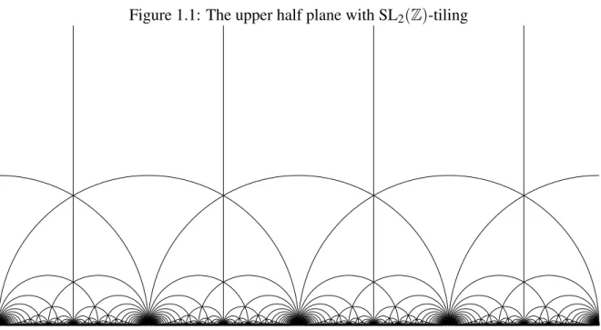
Figure 1.1: The upper half plane with SL2(Z)-tiling
group
γ
±
1 0
h 1
:h∈Z
γ−1.
Definition 1.1. LetΓ<SL2(Z) be a subgroup of finite index and consider a cuspγ∞ with
γ∈SL2(Z). Then thewidthofγ∞with respect toΓ, or the width ofγ∞inΓ\H∗, is defined as the smallest positive integerhfor which at least one ofγ
1 0
h
1
γ−1and −γ
1 0
h
1
γ−1is
inΓ.
Figure 1.1 is a useful picture to keep in mind when thinking about these things. It shows a tiling of the upper half plane along the SL2(Z)-action. Each tile here is an SL2(Z)-translate
of thefundamental domain
F :=
z∈H:−1
2 ≤ℜz≤ 1
2 and|z| ≥1
.
Sometimes in the literature parts of the boundary are left out in order thatF contain exactly one point of each orbit of the SL2(Z)-action onH. We will not worry about sets of measure zero here; our definition enables us to view the topological space SL2(Z)\Has a quotient
space ofF.
We can also use formula (1.1) to define an action of GL+2(R) onH or of GL+2(Q) on H∗. Here the superscript+means that we take the subgroup consisting of matrices with positive determinant.
We topologiseH∗in the following way: we take the usual topology onHbut a basis of open neighbourhoods for each cuspγ∞withγ ∈SL2(Z)consists of the sets
whereMruns throughR>0. With this topology, the set of cusps is discrete inH∗.
Definition 1.2. Let Γ be a subgroup of SL2(Z) of finite index and let k be an integer. A
modular form of weight k forΓis a holomorphic function f :H→Csatisfying the following
conditions:
• f(azcz++db) = (cz+d)kf(z)for all
a c b d
∈Γand allz∈H.
• f is holomorphic at the cusps. This means that for any matrix
a c b d
∈SL2(Z), the
function (cz+d)−kf(czaz++db) should be bounded in the region {z∈ C:ℑz≥M} for
some (equivalently, any)M>0.
The former condition is called themodular transformation propertyof f.
IfΓ<SL2(Z)is of finite index, then the set of modular forms of weightkfor the groupΓis
denoted byMk(Γ). Under the usual addition and scalar multiplication of functions,Mk(Γ)is aC-vector space; it can in fact be shown to be of finite dimension.
We will often focus on thecuspidal subspace Sk(Γ) of Mk(Γ) that is defined as the set of f ∈Mk that vanish at the cusps. By ”vanishing at the cusps” we mean that
lim
ℑz→∞
(cz+d)−kf
az+b cz+d
=0
should hold for allac bd∈SL2(Z). Elements ofSk(Γ)are calledcusp forms.
Now, letN∈Z>0be given. Define the subgroupΓ(N)of SL2(Z)by
Γ(N):=
a
c b
d
∈SL2(Z):
a c b d ≡ 1 0 0 1 modN .
Clearly, Γ(N) has finite index in SL2(Z) because it is the kernel of the reduction map
SL2(Z)→SL2(Z/NZ). A subgroup Γ of SL2(Z) that contains Γ(N) for some N will be
called acongruence subgroup of SL2(Z). If Γis a congruence subgroup then the smallest
positive integer N for which Γ⊃Γ(N) holds is called the level of Γ. Likewise, if f is a
modular form for some congruence subgroup, we define its level to be the smallest positive integerNsuch that f is modular for the groupΓ(N).
Many special types of congruence subgroups of some levelNturn out to be very interesting. Arguably, the two most interesting ones are
Γ0(N):=
a c b d
∈SL2(Z):
a c b d ≡∗ 0 ∗ ∗ modN and
Γ1(N):=
a c b d
∈SL2(Z):
One of the reasons to focus on these groups is that any modular form f of level N can be transformed into a modular form for Γ1(N2) (and the same weight) by replacing it with
f(Nz). In fact we have an isomorphism
Mk(Γ(N))∼=Mk Γ0(N2)∩Γ1(N)
⊂Mk(Γ1(N2)) (1.2)
defined by f(z)7→ f(Nz).
Note that we have
1 0 1 1
∈Γ1(N) for all N. If we plug this matrix into the transformation property of a modular form f ∈Mk(Γ1(N)), then f(z+1) = f(z)follows. In other words, f is periodic with period 1. Hence f is a holomorphic function of
q=q(z):=e2πiz.
We therefore have a power series expansion
f(z) =
∑
n≥0
an(f)qn,
the so-calledq-expansion of f. The absence of terms with negative exponent is equivalent with f being holomorphic at∞. If f is a cusp form, then it vanishes at∞and hencea0(f) =0. Be aware of the fact thata0=0 does not in general imply that f is a cusp form because there are other cusps than∞. The function fromZ>0toCdefined byn7→an(f)has very interesting
arithmetic properties for many modular forms f, as we shall see later.
1.1.2
Example: modular forms of level one
Let us give some examples of modular forms of level one now, that is modular forms for the full group SL2(Z). Note that SL2(Z)is generated by the matrices
1 0 1 1
and01−01. So to
check the modular transformation properties in this case it suffices to check f(z+1) = f(z)
and f(−1/z) =zkf(z).
Another interesting thing to observe here is thatz∈Hdefines a lattice
Λz:=Zz+Z⊂C.
Forz,w∈H there is a λ ∈C× with Λz =λΛw if and only if there is a γ ∈SL2(Z) with
z=γ(w). On the other hand, given a lattice Λ ⊂C we can choose a basis ω1,ω2 with
ℑ(ω2/ω1)>0. Then we haveΛ=ω1Λω2/ω1. This gives us a bijective correspondence
be-tween the SL2(Z)-equivalence classes ofHand theC×-equivalence classes of the set of rank
2 lattices inC.
a c
b d
∈SL2(Z) and allz∈H. Then we define the functionF =Ff from the set of rank 2
lattices inCtoCby
F(Zω1+Zω2):=ω1−kf(ω2/ω1) whereℑ(ω2/ω1)>0.
This functionF then satisfiesF(λΛ) =λ−kF(Λ)for allλ ∈Cand allΛ. Conversely, given
a functionF from the set of rank 2 lattices inCtoCthat satisfiesF(λΛ) =λ−kF(Λ)for all λ ∈Cand allΛ, we define f = fF by
f(z) =F(Zz+Z).
The function f will then satisfy the weight k modular transformation property for SL2(Z)
and in fact the assignments f 7→Ff andF7→ fF are inverse to each other.
Eisenstein series
Now that we have given definitions of modular forms, it becomes time that we write down some explicit examples. Let us first note that there are no non-zero modular forms of odd weight and level one; this can be seen by plugging in the matrix−01−01, which yields the
identity f(z) = (−1)kf(z). So if we want to write down a modular form we should at least do this in even weight. For reasons that we will make clear later, there cannot exist nonzero modular forms of negative weight and no non-constant modular forms of weight 0. Also, in level one there are no non-zero modular forms of weight 2.
Ifk≥4 is even, then
Gk(z) := (k−1)!
2(2πi)k
∑
0
m,n∈Z
1
(mz+n)k (1.3)
is a modular form of weightk, the so-called normalised Eisenstein series of weightk and level one (priming the summation sign here means that we ignore the terms whose denom-inator is equal to zero). One can in fact write downGk(z)in terms of lattices. The formula becomes then
Gk(Λ) = (k−1)!
2(2πi)k
∑
0
z∈Λ
z−k
and we readily see that it does satisfy the weight k modular transformation property for SL2(Z). The reason for using the normalisation factor(k−1)!/(2(2πi)k)becomes clear if
one writes down theq-expansion forGk:
Gk=−Bk
2k+n
∑
≥1σk−1(n)qn.
(1.4)
HereBkis thek-th Bernoulli number, defined by
x
ex−1 =
∑
k≥0Bk k!x
andσk−1(n)is defined as∑d|ndk−1.
We see that the arithmetic functionn7→σk−1(n)arises as the coefficients of a modular form, something that not everyone would expect right after reading the definition of a modular form.
Why can’t we takek=2 here? This is because the series (1.3) does not converge absolutely in that case and verifying the modular transformation property boils down to changing the order of summation. If we defineG2 by the q-expansion (1.4), then we get a well-defined holo-morphic function onHthat ’almost’ satisfies a modular transformation property for SL2(Z):
we have
G2
az+b cz+d
= (cz+d)2G2(z)−c(cz+d) 4πi
for all
a c
b d
∈SL2(Z). The ’almost’ modularity ofG2is still very useful within the theory of modular forms.
Discriminant modular form
The spacesMk(SL2(Z))fork∈ {4,6,8,10}can be shown to be one-dimensional, so they are
generated by Gk. In particular there are no non-zero cusp forms there. The lowest weight where we do have a cusp form of level one isk=12 (for higher levels, however, there are non-zero cusp forms of lower weight):
∆(z):=8000G34−147G26=q
∏
n≥1
(1−qn)24.
This form is called thediscriminant modular formormodular discriminantand it is a gen-erator for the spaceS12(SL2(Z)). If we write it out as a series
∆(z) =
∑
n≥1
τ(n)qn=q−24q2+252q3−1472q4+4830q5−6048q6+· · ·
thenτ(n)is called theRamanujan tau function. The tau function will play an important role
in this thesis. Ramanujan observed some very remarkable properties of it. Among these properties, the following ones occur, which he was unable to prove.
• For coprime integersmandnwe haveτ(mn) =τ(m)τ(n).
• For prime powers we have a recurrenceτ(pr+1) =τ(p)τ(pr)−p11τ(pr−1).
• For all prime numbers pwe have the estimation|τ(p)| ≤2p11/2.
The first two of these properties were proved by Mordell in 1917; they determineτ(n)in
terms ofτ(p)for pprime. The third property was proved by Deligne in 1974; its proof uses
Other properties found by Ramanujan and improved by others (cf. [83, Section 1] and [64, Section 4.5]) are congruence properties. For `∈ {2,3,5,7,23,691} there exist simple formulas forτ(n)modulo`or a power of`. The following summarises what is known about
this for`6=23:
τ(n)≡σ11(n) mod 211 forn≡1 mod 8,
τ(n)≡1217σ11(n) mod 213 forn≡3 mod 8,
τ(n)≡1537σ11(n) mod 212 forn≡5 mod 8,
τ(n)≡705σ11(n) mod 214 forn≡7 mod 8,
τ(n)≡n−610σ1231(n) mod 36 forn≡1 mod 3,
τ(n)≡n−610σ1231(n) mod 37 forn≡2 mod 3,
τ(n)≡n−30σ71(n) mod 53 forn6≡0 mod 5,
τ(n)≡nσ9(n) mod 7 forn≡0,1,2,4 mod 7,
τ(n)≡nσ9(n) mod 72 forn≡3,5,6 mod 7,
τ(n)≡σ11(n) mod 691 for alln.
Modulo 23 we have the following congruences forp6=23 prime:
τ(p)≡0 mod 23 if 23p=−1,
τ(p)≡σ11(p) mod 232 if pis of the forma2+23b2,
τ(p)≡ −1 mod 23 otherwise.
Later in this thesis we will studyτ(p)mod`for other values of`.
1.1.3
Eisenstein series of arbitrary levels
Having seen some examples in level one, we now turn back to the subgroups Γ0(N) and
Γ1(N)of SL2(Z). In this subsection we will define what Eisenstein series are for these
sub-groups. The situation is analogous to the level one case, though slightly more complicated. We will make use of Dirichlet characters, which will in this subsection be assumed to be primitive and take values in C×. If a Dirichlet character is evaluated at an integer not
co-prime with its conductor, then the value is defined to be 0. Details for this subsection can be found in [25, Chapter 4].
The casek≥3
ForN∈Z>0,k∈Z≥3andc,d∈Z/NZwe define
G(kc,d)(z):=
∑
0m≡cmodN n≡dmodN
1
(mz+n)k. (1.5)
This defines a modular form of weightkforΓ(N).
To get forms with nice q-expansions, we have to take suitable linear combinations of the
that satisfy the conditions
N(ψ)N(φ)|N and ψ(−1)φ(−1) = (−1)k. (1.6)
We then define
Gψk,φ := (−N(φ))
k(k−1)!
2(2πi)kg(φ−1)
N(ψ)
∑
c=1
N(φ)
∑
d=1
N(ψ)
∑
e=1
G(kcN(ψ),d+eN(ψ)),
where the pair (cN(ψ),d+eN(ψ)) is an element of (Z/(N(ψ)N(φ)Z))2 and for any C
-valued Dirichlet characterχ, the numberg(χ)denotes its Gauss sum:
g(χ):=
∑
ν∈(Z/N(χ)Z)×
χ(ν)exp
2πiν
N(χ)
. (1.7)
Theq-expansion ofGψk,φ is as follows:
Gψk,φ =−δ(ψ)Bk,φ
2k +n
∑
≥1σψ,φ k−1(n)q
n,
(1.8)
whereδ(ψ)equals 1 ifψ is trivial and 0 otherwise,Bk,φ is a so-called generalised Bernoulli
number defined by
∑
ν∈(Z/N(φ)Z)×
φ(n) xe
νx
eN(φ)x−1 =
∑
k≥0Bk,φ
k! x
k
andσkψ−,φ1(n)is a character-twisted sum of(k−1)-st powers of divisors, defined as
σkψ−,φ1(n) =
∑
d|n
ψ(n/d)φ(d)dk−1.
The functionGψk,φ is called anormalised Eisenstein series with charactersψ andφ. It is an
element ofMk(Γ1(N(ψ)N(φ))). In particular, it is an element ofMk(Γ1(N))and the same holds forGψk,φ(dz)for everyd| N( N
ψ)N(φ). Furthermore,G
ψ,φ
k is inMk(Γ0(N))if and only if the characterψ φ is trivial.
The casesk=1andk=2
Recall from the level one situation thatG2, defined by a q-series, is not a modular form, though it is not really far from being one. A similar picture occurs in arbitrary level: the series (1.5) do not converge absolutely fork∈ {1,2}, but the q-series (1.8) do define holo-morphic functions onHthat are ’almost’ modular. In fact it will turn out to be much nicer than it seems to be at first sight. Assumek∈ {1,2}, take N∈Z>0 and letψ andφ beC×
Let us first treat the casek=2. DefineGψ2,φ by theq-series (1.8). ThenG2ψ,φ is inM2(Γ1(N))
unless bothψ andφ are trivial, in which caseGψ2,φ(z)−dG2ψ,φ(dz) =G2(z)−dG2(dz)is in M2(Γ1(N))for alld|N. Again, the series is modular forΓ0(N)if and only ifψ φ is trivial.
In weight 1 the convergence problems of (1.5) are even worse but still we can do almost the same thing. We alter the definition of theq-series slightly: put
Gψ1,φ :=−δ(φ)B1,ψ+δ(ψ)B1,φ
2 +n
∑
≥1σψ,φ
0 (n)q
n.
This turns out to be a modular form inM1(Γ1(N))in all cases.
Eisenstein subspace
Now that we have defined for each spaceMk(Γ1(N))what its Eisenstein series are, we will define itsEisenstein subspaceas the subspace generated by these series:
Definition 1.3. Let k and N be positive integers with k 6=2. The Eisenstein subspace Ek(Γ1(N))ofMk(Γ1(N))is defined as the subspace generated by the modular formsGψk,φ(dz) defined above where(ψ,φ) runs through the set of pairs of Dirichlet characters satisfying
(1.6) and for given(ψ,φ), the numberd runs through all divisors ofN/(N(ψ)N(φ)).
Definition 1.4. LetNbe a positive integer. The Eisenstein subspaceE2(Γ1(N))ofM2(Γ1(N)) is defined as the subspace generated by the following modular forms:
• The formsGψk,φ(dz)defined above where(ψ,φ)runs through the set of pairs of
Dirich-let characters that are not both trivial and that satisfy (1.6) and for given (ψ,φ), the
numberdruns through all divisors ofN/(N(ψ)N(φ)).
• The formsG2(z)−dG2(dz)whered runs through divisors ofN, exceptd=1.
The given generators for the spaces actually do give a basis for each space, provided that in the casek=1 we take each formGψ1,φ =G1φ,ψonly once. Furthermore, we defineEk(Γ0(N)) to beMk(Γ0(N))∩Ek(Γ1(N))and this is actually generated by the Eisenstein series that lie inMk(Γ0(N)).
The Eisenstein subspace satisfies a very nice property:
Theorem 1.1. Let k and N be positive integers and letΓbe either Γ0(N)or Γ1(N). Then every f ∈Mk(Γ)can be written in a unique way as g+h with g∈Ek(Γ)and h∈Sk(Γ).
1.1.4
Diamond and Hecke operators
The arithmetic structure of modular forms turns out to be related to interesting operators on the spacesSk(Γ1(N)), called diamond operatorsandHecke operators. The operators are in fact defined on all ofMk(Γ1(N)), preservingEk(Γ1(N))as well. However, the treatments for Sk andEkdiffer at a few points and since we more or less ’know’Ek already, we will stick to Sk(Γ1(N))from now. Details for this subsection can be found in [25, Chapter 5].
Most operators on modular forms can be formulated in terms of a notation called theslash operator. For k∈Z and γ =
a c
b d
∈GL+2(R) we define the following operation on the space of functions f :H→C:
(f|kγ) (z):=det(γ)k−1(cz+d)−kf(γz).
It must be noted that in the literature there appears to be no consensus about the normalisa-tion factor det(γ)k−1; some textbooks use det(γ)k/2 instead. For a function f the modular
transformation property of weightkforΓ<SL2(Z)can be formulated in terms of the slash
operator as f|kγ = f for allγ ∈Γ. Be aware of the fact that slash operators in general don’t
leave the spacesSk(Γ)invariant.
Diamond operators
Note thatΓ1(N)is a normal subgroup ofΓ0(N)and that for the quotient we have
Γ0(N)/Γ1(N)∼= (Z/NZ)× by
a
c b
d
7→d. (1.9)
It follows from this normality that γ ∈Γ0(N) leaves the spaces Sk(Γ1(N)) invariant under the weightkslash action. Since the action of the subgroupΓ1(N)is trivial so this defines an action of(Z/NZ)× onSk(Γ1(N)):
hdif := f|k
a c
b d
,
where we can choose any matrixac bd∈Γ0(N)mapping todunder (1.9). The operatorhdi is called adiamond operator.
Letε :(Z/NZ)×→C× be a character. Then we define the subspaceSk(N,ε)ofSk(Γ1(N)) as
Sk(N,ε):=f ∈Sk(Γ1(N)):hdif =ε(d)f for alld∈(Z/NZ)×
and call it the ε-eigenspace of Sk(Γ1(N)). Note that if ε is the trivial character, then we
have Sk(N,ε) =Sk(Γ0(N)). If f ∈Sk(Γ1(N)) lies inside Sk(N,ε) then we say that f is a
representation of(Z/NZ)× on a finite-dimensionalC-vector space and thus is a direct sum of irreducible representations, hence we have
Sk(Γ1(N)) =
M
ε:(Z/NZ)×→C×
Sk(N,ε).
Note that we always haveh−1i= (−1)k so that Sk(N,ε) can only be non-zero for ε with ε(−1) = (−1)k.
Hecke operators
Congruence subgroups of SL2(Z)have the property that any two of them are commensurable,
which means that their intersection has finite index in both of them. Also, for any congruence subgroupΓ<SL2(Z)and anyγ ∈GL+2(Q)we have thatγ−1Γγ∩SL2(Z)is a congruence
subgroup of SL2(Z)and that γ−1Γγ is commensurable with Γ. It follows that for any two
congruence subgroupsΓ1 and Γ2 and any γ ∈GL+2(Q) the left action of Γ1 onΓ1γΓ2 has only a finite number of orbits. If we choose representativesγ1, . . . ,γr ∈GL+2(Q) for these
orbits then the operator
Tγ=TΓ1,Γ2,k,γ :Sk(Γ1)→Sk(Γ2) given by
Tγf = r
∑
i=1
f|kγi (1.10)
is well-defined and depends only on the double cosetΓ1γΓ2. Note that the diamond operator hdiis equal toTγ if we chooseγ∈Γ0(N)with lower right entry congruent todmodN.
Now, letpbe a prime number and consider the operatorTponSk(Γ1(N))defined as
Tp:=Tγ forγ =
1 0 0 p .
It is this operator that we call aHecke operator. If we write it out according to the definition ofTγthen we have
Tpf = (hpif)
k p 0 0 1 +
p−1
∑
j=0 f k 1 0 j p , (1.11)
where we take the conventionhpif =0 for p|N. It can be shown that the Hecke operators onSk(Γ1(N)) commute with the diamond operators and with each other. In particular the subspacesSk(N,ε)are preserved; hence we can speak of Tp as operators onSk(N,ε), with
Sk(Γ0(N))being a special case of this. The formula (1.11) then becomes
Tpf =ε(p)f
k p 0 0 1 +
p−1
∑
j=0 f k 1 0 j p ,
If we use the lattice interpretation for the level one case, we can formulate Tp in terms of
lattices. Take f ∈Sk(SL2(Z))and letF be the corresponding function on the set of full rank
lattices inC. Then the function corresponding toTpf is equal to
TpF(Λ) =pk−1
∑
Λ0⊂Λ
[Λ:Λ0]=p
F(Λ0), (1.12)
i.e. we sum over all sublattices of index p. A similar interpretation exists in arbitrary levels; we shall address this later, in Subsection 1.2.5.
We can also define operatorsTnfor arbitrary positive integersn. We do this by means of a
recursion formula:
T1=1,
Tmn=TmTn form,ncoprime,
Tpr=Tpr forp|N prime andr∈Z>1, Tpr+1 =TpTpr− hpipk−1T
pr−1 forp-N prime andr∈Z>0.
(1.13)
One motivation for this definition is that in the lattice interpretation formula (1.12) we can simply replacepwithn.
We can in fact describe the Hecke operators in terms ofq-expansions. Take N∈Z>0 and f ∈Sk(Γ1(N)). For alln∈Z>0we have
am(Tnf) =
∑
d|gcd(m,n)
gcd(d,N)=1
dk−1amn/d2(hdif).
This formula has some interesting special cases. First of all, form=1 we get
a1(Tnf) =an(f). (1.14)
Also, forpprime and f ∈Sk(N,ε)we have
an(Tpf) =
apn(f) forp-n,
apn(f) +ε(p)pk−1an/p(f) forp|n.
Petersson inner product
Let Γ<SL2(Z) be of finite index. We can define an inner product (i.e. a positive
def-inite hermitian form) on Sk(Γ) that is very natural in some sense. If we write z=x+iy then the measureµ :=dxdy/y2is GL+2(R)-invariant onHand the integralRΓ\Hµ converges
to [PSL2(Z): PΓ]π/3. The measure µ is called the hyperbolic measure on H. Also, for
f ∈Sk(Γ)the function|f(z)|2ykisΓ-invariant and bounded onH, hence the measure
is a Γ-invariant measure on H such that the integral RΓ\Hµf converges to a positive real
number. Now we define the Petersson inner product onSk(Γ)as follows:
(f,g):= 1 [PSL2(Z): PΓ]
Z
Γ\H
f(z)g(z)yk−2dxdy (1.15)
for f,g∈Sk(Γ), i.e. it is a scaled inner product associated to the Hermitian form f 7→R
Γ\Hµf.
The normalisation factor[PSL2(Z): PΓ]−1is used so that the value of the integral does not
depend on the chosen groupΓfor which f andgare modular.
We can in fact use the formula (1.15) for the Petersson inner product to define a sesquilinear pairing onMk(Γ)×Sk(Γ)(note that this would not work on Mk(Γ)×Mk(Γ)as the integral diverges there). ForΓ∈ {Γ0(N),Γ1(N)}the set of f ∈Mk(Γ)with(f,g) =0 for allg∈Sk(Γ)
is exactly the Eisenstein subspaceEk(Γ)defined in Subsection 1.1.3.
From now on, we return to the caseΓ=Γ1(N). The Petersson inner product behaves partic-ularly nicely with respect to the Hecke operators. Takeγ ∈GL+2(Q). Then the adjoint ofTγ
with respect to the Petersson inner product is equal toTγ∗ where
γ∗=
d −c
−b a
forγ =
a c
b d
,
i.e.
(Tγf,g) = (f,Tγ∗g) whereTγ∗=Tγ∗. For the diamond operators this boils down to
hdi∗=hdi−1
If we now letWN be the operator f 7→N1−k/2f|k
0
N
−1 0
onSk(Γ1(N))then we have
Tn∗=WNTnWN−1. (1.16)
We will study the operator WN in more detail in Subsection 1.1.7. In the special case gcd(n,N) =1 formula (1.16) simplifies to
Tn∗=hni−1Tn if gcd(n,N) =1.
In particular forncoprime toNthe operatorsTnandTn∗commute.
Hecke algebra
The diamond and Hecke operators on Sk(Γ1(N)) generate a subring of EndCSk(Γ1(N))
Tnwith gcd(n,N) =1. If confusion could arise we will writeTk(N)andT0k(N)respectively.
The structure ofT is important in the study ofSk(Γ1(N)). It can be shown thatT is a free
Z-module of rank dimSk(Γ1(N)). Consider the pairing
T×Sk(Γ1(N))→C, (T,f)7→a1(T f).
For any ring A we put TA :=T⊗A. From formula (1.14) it follows immediately that the
induced pairingTC×Sk(Γ1(N))→Cis perfect. In particular we have
Sk(Γ1(N))∼=HomZ−Mod(T,C) (1.17)
Under this isomorphism, the action ofTonSk(Γ1(N))comes from the following action ofT
on HomZ−Mod(T,Z): letT ∈Tsendφ ∈HomZ−Mod(T,Z)toT
07→
φ(T T0). It can be shown
that Hom(TQ,Q) is in this way a free TQ-module of rank one so that in fact Sk(Γ1(N))is free of rank one as aTC-module. For each subringAofC, we can identify HomZ−Mod(T,A)
with theA-module of modular forms whoseq-expansion has coefficients inA.
1.1.5
Eigenforms
The commutativity of all theTn,Tn∗,hdiandhdi∗fornanddcoprime toN has an interesting
consequence:
Theorem 1.2. For k,N∈Z>0the space Sk(Γ1(N))has a basis that is orthogonal with respect to the Petersson inner product and whose elements are eigenvectors for all the operators in
T0.
Theorem 1.2 would fail if we took all the Hecke operators in T, i.e. also the Tn with gcd(n,N)>1. This is because those operators are in general not semi-simple, so we do not get a decomposition of our vector space into eigenspaces. Forms that are eigenvectors for all the operators inTare calledeigenforms. If a form is an eigenvector for all the operators inT0, we will call it aT0-eigenform. EachT0-eigenform is an eigenvector for the diamond operators, so must lie inside some spaceSk(N,ε). An eigenform f is called normalisedif
a1(f) =1. From (1.14) and the commutativity ofTit follows easily that f ∈Sk(Γ1(N))is a normalised eigenform if and only if the mapT→Ccorresponding to f as in (1.17) is a ring homomorphism.
ConsiderMandN withM|N. For each divisord ofN/Mwe have a map
αd:Sk(Γ1(M))→Sk(Γ1(N)) defined by f(z)7→ f(dz).
The map αd is called a degeneracy map. Note that for d =1 it is just the inclusion of
Sk(Γ1(M))intoSk(Γ1(N)). The subspace ofSk(Γ1(N))generated by all theαd(f)forM|N,
M<N,d|N/Mis called theold subspaceofSk(Γ1(N))and is denoted bySk(Γ1(N))old.
Theorem 1.3. Let f ∈Sk(Γ1(N))new be an eigenform. Then C· f is an eigenspace of
Sk(Γ1(N))and a1(f)6=0. Furthermore, Sk(Γ1(N))newis generated by its eigenforms.
This is called themultiplicity one theorem. In fact, in the new subspace there is no distinction between eigenforms forTand eigenforms forT0. The theorem allows us to put the normali-sationa1=1 on eigenforms in the new subspace. New eigenforms f that satisfya1(f) =1 are callednewforms. If we combine this with (1.14) then we see
Theorem 1.4. Let N and k be positive integers and let f ∈Sk(Γ1(N))be a newform. Then the eigenvalue of the Hecke operator Tnon f is equal to the q-coefficient an(f).
If f ∈ Sk(Γ1(M)) a T0k(M)-eigenform, then for all d the form αd(f)∈ Sk(Γ1(dM)) is a
T0k(dM)-eigenform. We furthermore have a decomposition:
Sk(Γ1(N)) =
M
M|N
M
d|N M
αd(Sk(Γ1(M))new)
that allows us to write down an interesting basis forSk(Γ1(N)):
Theorem 1.5. Let N and k be given positive integers. Then the following set is a basis for Sk(Γ1(N))consisting ofT0-eigenforms.
[
M|N
[
d|N M
{αd(f): f is a newform in Sk(Γ1(M))}.
The fieldKf
If f ∈Sk(Γ1(N))is a newform with characterε, then the values ofε together with the coef-ficientsan(f)generate a field
Kf :=Q(ε,a1(f),a2(f), . . .)
which is known to be a number field. It can be shown that for any embeddingσ :Kf ,→C
the functionσf :=∑σ(an)qn is a newform inSk(Γ1(N))with character σ ε. To a newform f ∈Sk(N,ε)we can attach a ring homomorphism
θf :T→Kf
defined by
θf(hdi) =ε(d) and θf(Tp) =ap,
as in (1.17). We define
If :=ker(θf),
which is a prime ideal ofTcalled theHecke idealof f. It is known that imθf is an order in
1.1.6
Anti-holomorphic cusp forms
From time to time we will also be considering anti-holomorphic cusp forms. A function f :H→Cis called an anti-holomorphic cusp form of some levelN and weightkifz7→ f(z)
is inSk(Γ1(N)). The space of anti-holomorphic cusp forms of levelNand weightkis denoted bySk(Γ1(N)). We let the diamond and Hecke operators act onSk(Γ1(N))by the formulas
hdif =hdif and Tpf =Tpf,
where we denote by f the functionz7→ f(z). The spacesSk(N,ε)are now defined as
Sk(N,ε) =f : f ∈Sk(N,ε)
=f ∈Sk(Γ1(N)):hdif =ε(d)f for alld∈(Z/NZ)× .
If we have a simultaneous eigenspace insideSk(Γ1(N))for the diamond and Hecke operators then we also have an eigenspace with conjugate eigenvalues and of the same dimension (which could be the same space if all these eigenvalues are real). It follows that we have a decomposition of Sk(Γ1(N))⊕Sk(Γ1(N)) into eigenspaces with the same eigenvalues as in the decomposition ofSk(Γ1(N)), but the dimension of each such eigenspace is twice the dimension of its restriction toSk(Γ1(N)).
1.1.7
Atkin-Lehner operators
The main reference for this subsection is [3].
Besides diamond and Hecke operators, there is another interesting type of operators on Sk(Γ1(N)), namely theAtkin-Lehner operators. Let Q be a positive divisor ofN such that gcd(Q,N/Q) =1. LetwQ∈GL+2(Q)be any matrix of the form
wQ=
Qa
Nc b
Qd
(1.18)
witha,b,c,d∈Z and det(wQ) =Q. The assumption gcd(Q,N/Q) =1 ensures that such a wQ exists. A straightforward verification shows f|kwQ∈Sk(Γ1(N))). Now, given Q, this f|kwQ still depends on the choice ofa,b,c,d. However, we can use a normalisation in our
choice ofa,b,c,d which will ensure that f|kwQonly depends onQ. Be aware of the fact that different authors use different normalisations here. The one we will be using is
a≡1 modN/Q, b≡1 modQ, (1.19)
which is the normalisation used in [3]. We define
WQ(f):=Q1−k/2f|kwQ=
Qk/2
(Ncz+Qd)k f
Qaz+b Ncz+Qd
, (1.20)
An unfortunate thing about these Atkin-Lehner operators is that they do not preserve the spacesSk(N,ε). But we can say something about it. Letε :(Z/NZ)×→C× be a character
and suppose that f ∈Sk(N,ε). By the Chinese Remainder Theorem, one can writeε in a
unique way asε =εQεN/Q such thatεQis a character on(Z/QZ)× and εN/Qis a character
on(Z/(N/Q)Z)×. It is a fact that
WQ(f)∈Sk(N,εQεN/Q).
Also, there is a relation between theq-expansions of f andWQ(f):
Theorem 1.6. Let f ∈Sk(N,ε)be a newform. Take Q|N withgcd(Q,N/Q) =1. Then
WQ(f) =λQ(f)g
withλQ(f)∈Can algebraic number of absolute value 1 and g∈Sk(N,εQεN/Q)a newform.
Suppose now that n is a positive integer and write n=n1n2 where n1consists only of prime factors dividing Q and n2consists only of prime factors not dividing Q. Then we have
an(g) =εN/Q(n1)εQ(n2)an1(f)an2(f).
The numberλQ(f)in the above theorem is called apseudo-eigenvaluefor the Atkin-Lehner
operator. In some cases there exists a closed expression for it.
Theorem 1.7. Let f ∈Sk(N,ε)be a newform and suppose q is a prime that divides N exactly
once. Then we have
λq(f) =
g(εq)q−k/2aq(f) ifεqis non-trivial,
−q1−k/2a
q(f) ifεqis trivial.
Here, g(εq)is the Gauss sum ofεq.
Theorem 1.8([2, Theorem 2]). Let f∈Sk(N,ε)be a newform with N square-free. For Q|N
we have
λQ(f) =ε(Qd−
N Qa)
∏
q|Q
ε(Q/q)λq(f).
Here, a and d are defined by (1.18). Moreover, this identity holds without any normalisation assumptions on the entries of wQ, as long as we defineλq(f)by the formula given in Theorem
1.7.
1.2
Modular curves
1.2.1
Modular curves over
C
LetΓ<SL2(Z)be a subgroup of finite index. If one divides out the group action ofΓonH
one obtains a Riemann surface
YΓ:=Γ\H.
If we add the cusps toYΓ and use(q|0γ−1)1/w(γ∞) as a local parameter at the cusp γ∞ we obtain another Riemann surface
XΓ:=Γ\H∗,
which happens to be compact. This compactness implies thatXΓis in fact (the analytification of) a projective algebraic curve overC, the open subsetYΓ⊂XΓ being an affine curve.
ForΓequal toΓ0(N),Γ1(N)orΓ(N)we writeYΓ asY0(N),Y1(N)orY(N)andXΓasX0(N), X1(N)orX(N)respectively. These are the curves in which we are primarily interested.
The curvesY0(N), Y1(N) andY(N) have moduli interpretations. Take z∈H and consider the lattice Λz =Zz+Z, as we did in Subsection 1.1.2. Then C/Λz is a complex elliptic
curve and in this way SL2(Z)\H is in bijection with the set of all isomorphism classes of
elliptic curves overC. This gives in all three cases the moduli interpretation forN =1. In general,Y0(N)(C) =Γ0(N)\H is in bijection with the set of isomorphism classes of pairs
(E,C) whereE is an elliptic curve over CandC⊂E(C) is a cyclic subgroup of orderN. The bijection is obtained by
z7→(C/Λz,
1
NZmodΛz).
The additional informationCthat we attach toEis called alevel structure.
Likewise, forY1(N)(C) =Γ1(N)\Hthe map
z7→(C/Λz,
1
N modΛz).
defines a bijection with the set of isomorphism classes of pairs(E,P)withEan elliptic curve overCandP∈E(C)a point of orderN.
To describe the moduli interpretation ofY(N), we use the Weil pairing on elliptic curves over
C. The sign convention we use is such that the Weil eN-pairing on theN-torsion ofC/Λis
defined as
eN(z,w) =exp
πiN zw−zw
covol(Λ)
. Then the map
z7→(C/Λz,
1
NmodΛz, z
NmodΛz)
defines a bijection between Y(N)(C) = Γ(N)\H and the set of isomorphism classes of triples(E,P,Q)where E is an elliptic curve overCandP,Q∈E(C)[N]are points that
In view of (1.2), the curveY(N) is isomorphic toYΓ with Γ=Γ0(N2)∩Γ1(N). The map z7→Nz defines an isomorphism YΓ →Y(N). In terms of moduli, YΓ parametrises triples
(E,C,P)withE/Can elliptic curve,C⊂E(C)cyclic of orderN2andP∈Ca point of order N. Let us describe what the given isomorphismYΓ →Y(N) sends (E,C,P) to. Choose a generatorP0forCwithP=NP0and aQ∈E(C)[N2]witheN2(P0,Q) =exp(2πi/N2). Then
the image of(E,C,P)is the triple(E/hNPi,PmodNP,NQmodNP).
1.2.2
Modular curves as fine moduli spaces
In the previous subsection we spoke about bijections between points ofYΓ(C) and isomor-phism classes of elliptic curves with certain level structures. It turns out that this can be put in a more general setting, which is what we will do in the present subsection.
For an arbitrary schemeS, an elliptic curve over Sis defined to be a proper smooth group schemeE over S of which all the geometric fibres are elliptic curves. For a fixed positive integerN that we use for our level structures, we will usually work with schemes in which Nis invertible, i.e. schemes overZ[1/N], which is the treatment of [22]. Getting rid of this condition is done in the standard work [36] and makes things much more technical.
So letN be a positive integer, letS/Z[1/N]a scheme and letE/Sbe an elliptic curve. Then a point of orderNofE/Sis meant to be a sectionP∈E(S)[N]whose pull-back to all geometric fibres ofE/Sdefines a point of orderN. Define a contravariant functor
F1(N): SchZ[1/N]→Set
from the category of schemes over Z[1/N] to the category of sets as follows. We send a scheme S to the set of isomorphism classes of pairs (E,P) where E is an elliptic curve over S and P a point of order N of E/S. And we send a morphism T →S to the map F1(N)(S)→F1(N)(T)that sends every pair(E,P)/Sto its pull-back alongT →S.
Theorem 1.9 (Igusa). Let N >3 be an integer. Then there exists a smooth affine scheme Y1(N)overZ[1/N], an elliptic curveEover Y1(N)and a pointPofE/Y1(N)of order N that satisfies the following universal property: for all schemes S/Z[1/N] and pairs (E,P) with E/S an elliptic curve and P a point of order N of E/S there are unique morphisms S→Y1(N) and E→Esuch that the following diagram is commutative with Cartesian inner square:
E
/
/
E
S //
P
B
B
Y1(N)
P
[
[
Moreover, the geometric fibres of Y1(N)/Z[1/N]are irreducible curves.
Note that we abusively use the same notationY1(N) as in the previous subsection; we will write subscripts in cases where this abuse might lead to confusion. The scheme Y1(N)
S→Y1(N) defines a functorial bijection betweenY1(N)(S)and F1(N)(S). Because we can give such an isomorphism of functors, or equivalently, a universal(E,P), we say thatY1(N)
is afine moduli spacefor the functorF1(N).
The complex curveY1(N)from the previous subsection, together with its moduli description, is canonically isomorphic to the base changeY1(N)CofY1(N)Z[1/N]toC. In fact, overC, the universal elliptic curveEC/Y1(N)Ccan be described analytically as follows: ConsiderC×H
as line bundle overHand embedZ2×Hinto it by
Z2×H,→C×H, ((m,n),z)7→((mz+n),z).
Call the image of this embeddingΛ. The quotient(C×H)/Λ is an elliptic curveE overH
whose fibre overz∈HisC/Λz. The sectionP:H→E defined byz7→1/Nhas orderN. We
have an action of SL2(Z)onC×Has follows:
a c
b d
(w,z):=
w cz+d,
az+b cz+d
.
This action respectsΛ and therefore induces an action on E. The subgroup of SL2(Z)
re-specting the sectionPis exactlyΓ1(N)and we can in fact describeEC/Y1(N)Cas the quotient
ofE/Hby the action ofΓ1(N):
EC∼=Γ1(N)\((C×H)/Λ). (1.21)
Let us note that from Theorem 1.9 it follows thatY1(N)has a model overQand that for each field extensionK/Qthe setY1(N)(K)ofK-rational points ofY1(N)Q is in bijection with the set of isomorphism classes of pairs(E,P)whereE is an elliptic curve overK andP∈E(K)
is a K-rational point of orderN. We furthermore see that for p-N the curveY1(N)Q has a non-singular reductionY1(N)Fp that parametrises all pairs(E,P)with E an elliptic curve over a fieldK of characteristicpandP∈E(K)a point of orderN.
There is another functor that people sometimes use; this is the functor
Fµ(N): Sch→Set.
It takes a schemeSto the set of pairs(E,ι)whereE/Sis an elliptic curve andι:µN,S→Eis
a closed immersion of group schemes overS. There exists a fine moduli spaceYµ(N)/Z[1/N]
forFµ(N) as well. Also here we have an isomorphism ofYµ(N)C with the complex curve Y1(N)C; it is defined by sendingzto(C/Λz,exp(2πik/N)7→k/NmodΛ). In fact, we have
an isomorphism of schemes
Y1(N)∼=Yµ(N) (1.22)
immersion of group schemesι:µN,S→E0we have an endomorphism ofµN,Sthat is defined
by sendingQ∈µN,S(T)toeN(P,(ιQ)0)for anyS-schemeT, where(ιQ)0 denotes any point
ofE(T) that maps to ιQ along φ. We take for ι0 the ι that makes this endomorphism the
identity. OverCthe isomorphism (1.22) can be defined by sendingz∈HtowN(z) =−1/Nz.
ForY(N)with N >2 there is a similar description as the fine moduli space over Z[1/N]
parametrising all pairs(E/S,φ)whereφ :(Z/NZ)S→E(S)[N]is an isomorphism of group
schemes. In this case, theY(N) from the previous subsection is a disjoint union of φ(N)
copies of the base changeY1(N)C ofY1(N)Z[1/N] toC: one for each possible value of the
Weil pairing.
One cannot constructY0(N) as the fine moduli space parametrising pairs (E,C) of elliptic curve and cyclic subgroups of order N in any sensible meaning. The obstruction lies in the fact that such pairs always have the non-trivial automorphism−1. However, we can do the following. Let the groupG= (Z/NZ)× act on Y1(N) by letting d ∈(Z/NZ)× act as
(E,P)7→(E,dP) on moduli and define Y0(N) as the quotient G\Y1(N). AlthoughY0(N)
is not a fine moduli space, it is true that for all fieldsK with char(K)-N the setY0(N)(K) is naturally in bijection with the set of K-isomorphism classes of pairs (E,C) where E is an elliptic curve over K andC⊂E is a cyclic subgroup of orderN defined over K. Here as wellY0(N)from the previous subsection is canonically isomorphic to the base change of Y0(N)Z[1/N]toC.
1.2.3
Moduli interpretation at the cusps
In Subsection 1.2.1 we defined the compact Riemann surfacesX0(N), X1(N)andX(N)but so far we only gave moduli descriptions forY0(N),Y1(N)andY(N). In this subsection we will explain the approach of [22] to extend the moduli interpretation to the cusps.
N´eron polygons and generalised elliptic curves
Letnbe a positive integer and letkbe a field. AN´eron n-gon over kis defined to be a singu-lar connected curve overkthat can be constructed as follows: taken copies ofP1k, indexed byZ/nZ and identify for eachi∈Z/nZ the point ∞of the i-thP1 with the point 0 of the (i+1)-stP1such that this intersection point is an ordinary double point.
Fora∈P1
k(k)andi∈Z/nZwe denote the pointaof thei-thP1of a N´eronn-gon by(a,i).
The choice of projective coordinates onP1allows us to identifyP1k− {0,∞}withGm,k, which
acts onP1k by(a,b)7→ab. This way we give the smooth locusCsmof a N´eronn-gonCthe structure of a commutative group scheme, where addition is defined as
(a,i) + (b,j):= (ab,i+j). (1.23)
Note that a N´eron n-gonC together with its addition (1.23), admits an action of the group
µn(k)by lettingζ ∈µn(k)act as(a,i)7→(ζia,i). Furthermore, we have an automorphismι
defined on it that sends(a,i)to(a−1,−i). In fact
Aut(C,+)∼=µn(k)× hιi (1.24)
is the group of automorphisms ofCthat respect the addition.
We are now ready to define the notion of a generalised elliptic curve.
Definition 1.5. Let S be a scheme. Then a generalised elliptic curve over S is a scheme E over S that is proper, flat, of finite presentation that comes equipped with a morphism
Esm×SE
+
→E that makesEsm into a commutative group scheme acting onE and such that each geometric fibre ofE/Sis either an elliptic curve or a N´eron polygon equipped with an action as in (1.23).
Definition 1.6. IfE is a generalised elliptic curve over a schemeS, thena point of order N ofE/Sis meant to be section inEsm(S)[N]whose pull-back to all geometric fibres defines a point of orderNsuch that the subgroup generated by it meets all irreducible components.
The notion of generalised elliptic curves enables us to generalise Igusa’s theorem toX1(N):
Theorem 1.10(see [22, Chapter IV]). Let N>4be an integer. Then there exists a proper smooth scheme X1(N) overZ[1/N], a generalised elliptic curveE over X1(N) and a point
P of E/X1(N) of order N that satisfies the following universal property: for all schemes S/Z[1/N] and pairs (E,P) with E/S a generalised elliptic curve and P∈E(S) a point of order N there are unique morphisms S→X1(N)and E→Esuch that the following diagram is commutative with Cartesian inner square:
E
/
/
E
S //
P
B
B
X1(N)
P
[
[
Moreover, the geometric fibres of X1(N)/Z[1/N]are irreducible curves.
The schemeY1(N) is naturally an open subscheme ofX1(N) and the complement is called thecuspidal locus of X1(N). We can also extendYµ(N) to cusps and get a schemeXµ(N)
parametrising pairs(E,ι)of generalised elliptic curves over S together with closed
immer-sions ι:µN,S→E. We require that the image of ι meets the geometric fibres of E in all
components. The isomorphism (1.22) extends to an isomorphismX1∼=Xµ.
As with Y0(N), we define X0(N) by dividing out the group action of (Z/NZ)× defined by d :(E,P)7→(E,dP). Furthermore, there also exists for N >2 a scheme X(N) that is a fine moduli space for pairs (E,φ)/S/Z[1/N] with E/S a generalised elliptic curve and
φ :(Z/NZ)2S→Esma closed immersion ofS-group schemes meeting all irreducible
Tate curves
We will give an informal discussion on the Tate curve now. Precise results can be found in [22, Chapter VII]. See also [74, Chapter V] for a more elementary and explicit approach. The idea is that for an elliptic curveE=C/Λ overCwe haveE ∼=C×/qZ withq=exp(2πiz).
An explicit Weierstrass equation forE is
E:y2+xy=x3+a4(q)x+a6(q) (1.25)
with
a4(q) =−5
∑
n≥1
σ3(n)qn and a6(q) =− 1
12n
∑
≥1(5σ3(n) +7σ5(n))qn.
An isomorphismC×/qZ→Ecan be given by
t 7→
∑
n∈Z
qnt
(1−qnt)2−2
∑
n≥1
σ1(n)qn,
∑
n∈Z
(qnt)2
(1−qnt)3+
∑
n≥1
σ1(n)qn
!
,
where of course we sendt ∈qZto 0∈E. This isomorphism leads to the following
identifi-cation of differentials onC×/qZ andE:
dt
t = dx
2y+x.
We will use thist-coordinate notation whenever it makes sense.
The Weierstrass equation (1.25) defines a generalised elliptic curve overZ[[q]]. Also, for any w∈Z>0 we can regard (1.25) as a Weierstrass equation for an elliptic curve over the ring
Z((q1/w)). We call this the Tate curve Eqover Z[[q]]and Z((q1/w))respectively. The idea
is now that if we move our favourite cusp of widthwto∞and seeq1/w as a local parameter
there, thenEqcan be seen as a (formal completion of a) universal elliptic curve over a
punc-tured neighbourhood of our cusp. This can in fact be used to describe cusps ofX1(N)over arbitrary fields, not justC.
Let nowN >4 and wbe integers withw|N. Let kbe a field of characteristic not dividing N that contains allN-th roots of unity and put R=k[[q1/w]]andK =k((q1/w)). The N´eron model Eq of Eq over K is the smooth locus of a generalised elliptic curve over R whose
special fibreEqis a N´eronw-gon overk. We have canonical isomorphismsEq(K)∼=K×/qZ
and Eq,0(K)∼=R×/qZ, where the latter is the subset of Eq(K) consisting of points whose
specialisation lies in the 0-component of the smooth locus. The component group ofEqis
canonically isomorphic to
Eq(k)/E
0
q(k)∼=Eq(K)/Eq,0(K)∼= (q1/w)Z/qZ∼=Z/wZ.
Using the identification Eq(K)∼=K×/qZ we get an isomorphism from µ
N(k)×Z/wZ to
Eq(K)[N], hence a homomorphism toEq(k), defined by(ζ,i)7→ζqi/w. This gives us a
and a point(ζ,i)of orderNofEq(K)satisfying gcd(i,w) =1; this last condition is necessary
so as to meet the requirement that the subgroup generated by it meets all the components of the special fibre. Be aware of the fact that this does not lead to a unique notation for cusps because of (1.24).
Let us work out what this means for a cuspγ∞withγ =
a c
b d
∈SL2(Z)in the upper half
plane model forX1(N)C. Writez∈Has γ ω withω ∈Hand let w=w(γ) =N/gcd(c,N)
be the width ofγ∞in X1(N). If we putqγ =exp(2πiω)then q
1/w
γ is a local parameter for
X1(N)Catγ∞. The fibre of(E,P)abovez=γ ω is then uniquely isomorphic to
(E,P)z∼=
C/Λω,
cω+d
N
.
In terms of the parameterq1γ/wthis can be written as
(E,P)z∼=
C×/qZ,ζNdqcγ/N
=C×/qZ,ζd
N(q
1/w γ )
c/gcd(c,N),
where we have putζN =exp(2πi/N). Our conclusion is thatEγ∞ is the N´eronw-gon with
w=N/gcd(N,c)and for the point of orderNon it we have
Pγ∞=
exp(2πid/N), c
gcd(c,N)
.
Note that the cusp does not uniquely determine the numberd, but the different choices lead to isomorphic objects.
Let us note that in this way we can see that the cusp 0∈H∗is defined overQ: it corresponds to(c,d) = (1,0) and thus to anN-gon with the point (1,1) on it, which is invariant under the action of Gal(Q(ζN)/Q). The cusp ∞∈H∗ is not defined over Q: it corresponds to (c,d) = (0,1)and thus to a 1-gon with the point (ζN,0)on it, whose isomorphism class in
only invariant under the stabiliser subgroup ofQ(ζN+ζN−1).
1.2.4
Katz modular forms
The algebraic description of modular curves allows us to give an algebraic description of modular forms as global sections of certain line bundles over modular curves. These sec-tions are sometimes calledKatz modular formsand in particular they allow us to speak about modular forms forΓ1(N)over anyZ[1/N]-algebra.
LetS be a scheme and letE/S be a generalised elliptic curve. The curveE has a sheaf of relative differentialsΩ1E/Sas well as a zero section 0 :S→E. We put
ωE/S:=0∗Ω1E/S,
which is a line bundle onS. In particular, forN>4 andk∈Zwe can consider the line bun-dleω⊗k
EC/Y1(N)C on
in an analytic context, the sheafω((⊗k
C×H)/Λ)/H is a freeOH-module of rank 1, generated by
(dw)⊗k, wherewdenotes the coordinate on the factorC. In particular, any holomorphic func-tion f :H→Ccan be seen as the section f(z)(dw)⊗k ofω((⊗k
C×H)/Λ)/Hand vice versa. The
action ofγ =
a c b d
∈SL2(Z)on(C×H)/Λ sends f(z)(dw)⊗k to(cz+d)−kf(γz)(dw)⊗k.
Using that Γ1(N) acts freely on H, we see now that H0(Y1(N)(C),ω⊗k) is isomorphic to the space of holomorphic functions on Hthat satisfy the weight k modular transformation property forΓ1(N).
Now, we extend this toEC/X1(N)C. Global sections ofH0(X1(N)(C),ω⊗k)can still be seen
as holomorphic functions f :H→Csatisfying the weightkmodular transformation property forΓ1(N). Using the description of neighbourhoods of cusps as Tate curves, one can see that the extra condition at the cusps is simply that f has to be holomorphic at the cusps. So we have an isomorphism
Mk(Γ1(N))∼=H0
X1(N)C,ω
⊗k
EC/X1(N)C
.
Cusps forms are modular forms that vanish at the cusps, so we have
Sk(Γ1(N))∼=H0
X1(N)C,ω⊗k
EC/X1(N)C(
−cusps)
.
Here, cusps denotes the divisor of all cusps, all counted with multiplicity 1. The above isomorphisms inspire us to write down the definition of Katz modular forms
Definition 1.7. LetN>4 andk be integers. LetAbe aZ[1/N]-algebra. Then the space of Katz modular forms forΓ1(N)overAis defined to be theA-module
Mk(Γ1(N),A):=H0
X1(N)A,ωE⊗Ak/X1(N)A
and the space of Katz cusp forms overAis defined as theA-module
Sk(Γ1(N),A):=H0
X1(N)A,ωE⊗Ak/X1(N)A(−cusps)
.
Let us remark that there is an isomorphism of line bundles
ω⊗2
E/X1(N) ∼
−→Ω1X1(N)/Z[1/N](cusps),
called theKodaira-Spencer isomorphism, see [35, Subsection A1.3.17]. OverCit is defined by f(z)(dw)⊗27→(2πi)−1f(z)dz. It is compatible with base-change. A consequence of this
isomorphism is
S2(Γ1(N),A)∼=H0
X1(N)A,Ω1X
1(N)A/A
q-expansions
We can define theq-expansion of a Katz modular form of levelNand weightkalgebraically. Let A be an algebra over Z[1/N,ζN] and consider the Tate curve Eq over A[[q]] together
with the pointt=ζN modqZon it. By Theorem 1.10, the pair(Eq,ζNmodqZ)is the
base-change of E/X1(N)along an A[[q]]-valued point ofX1(N). This base-change gives a pull-back homomorphism
Mk(Γ1(N),A) =H0
X1(N)A,ωE⊗Ak/X1(N)A
→H0SpecA[[q]],ωE⊗k
q/A[[q]]
.
The latter object is a free module overA[[q]]generated by(dt/t)⊗k, wheredt/tis the standard differential onEq. So we obtain a homomorphism ofA-modules
Mk(Γ1(N),A)→A[[q]]
dt
t
⊗k
.
Applying this homomorphism and dropping the factor(dt/t)⊗kdefines for f ∈Mk(Γ1(N),A) itsq-expansion in A[[q]]. Formation of thisq-expansion commutes with base-change. Over
C thisq-expansion coincides with the usual q-expansion of f ∈Mk(Γ1(N)) since the pair
(Eq,ζNmodqZ)corresponds to a neighbourhood of the cusp∞.
A thorn in the eye here is that the ringAhas to contain a primitiveN-th root of unity, while we wish to work, for instance, overQ. Luckily, we can resolve this problem. So letAbe a
Z[1/N]-algebra. Remember that we have an isomorphism
X1(N)∼=Xµ(N). This induces an isomorphism
Mk(Γ1(N),A)∼=H0
Xµ(N),ω(⊗k
E/hPi)A/Xµ(N)A
.
Now, consider the pair(Eq,ι)over A[[q]]withι the canonical injection µN,A ,→Eq via the
t-coordinate. We repeat the above argument and obtain a map
Mk(Γ1(N),A)→A[[q]].
Over C, the q-series of f ∈Mk(Γ1(N),A) obtained in this way coincides with the usual q-expansion ofWN(f). So we have the following proposition:
Proposition 1.1. Let N and k be positive integers with N>4. Let A be a subring ofCin which N is invertible. Then the image of the canonical map
Mk(Γ1(N),A)→Mk(Γ1(N))