Copula Models
Philipp Arbenz, Mathieu Cambou, Marius Hofert, Christiane Lemieux, and Yoshihiro Taniguchi
Dedicated to Ian H. Sloan on the occasion of his 80th birthday.
Abstract An importance sampling approach for sampling from copula models is introduced. The proposed algorithm improves Monte Carlo estimators when the functional of interest depends mainly on the behaviour of the underlying random vector when at least one of its components is large. Such problems often arise from dependence models in finance and insurance. The importance sampling framework we propose is particularly easy to implement for Archimedean copulas. We also show how the proposal distribution of our algorithm can be optimized by making a connection with stratified sampling. In a case study inspired by a typical insur-ance application, we obtain variinsur-ance reduction factors sometimes larger than 1000 in comparison to standard Monte Carlo estimators when both importance sampling and quasi-Monte Carlo methods are used.
1 Introduction
Many applications in finance and insurance lead to the problem of calculating a functional of the formµ=E(Ψ0(XXX)), whereXXX= (X1, . . . ,Xd):Ω →Rdis a ran-dom vector on a probability space (Ω,F,P) andΨ0:Rd→R is a measurable function. If the components ofXXXcannot be assumed to be independent, it is popular
Philipp Arbenz SCOR
e-mail: [email protected]
Mathieu Cambou
Institute of Mathematics, Station 8, EPFL, 1015 Lausanne, Switzerland e-mail: [email protected]
Marius Hofert·Christiane Lemieux·Yoshihiro Taniguchi ( ) University of Waterloo, Waterloo, Ontario, Canada
e-mail: [email protected]; [email protected]; [email protected]
to model the distribution functionHofXXXwith a copulaC, such thatH(x1, . . . ,xd) = C(F1(x1), . . . ,Fd(xd)),xxx∈Rd, whereFj(x) =P(Xj≤x), j∈ {1, . . . ,d}, are the uni-variate margins of H andC:[0,1]d →[0,1]is a copula. A copula allows one to separate the dependence structure from the marginal distributions, which is useful for constructing multivariate stochastic models. We assume the reader to be familiar with copulas and refer to [15] or [17] for an introduction; see also Section 2 for important background information.
A drawback of using such flexible models is that an analytical form for the quan-tity of interestE(Ψ0(XXX))rarely exists, and thus numerical methods must be applied to evaluate it. Preferably, the employed techniques should be applicable to high-dimensional problems, which are common in finance. An advantage of Monte Carlo (MC) simulation is that the rate of convergence of its error is independent of the dimensionality of a given problem. Nevertheless, the convergence rate of plain MC is generally slow so that MC is often combined with some variance reduction tech-nique (VRT) to improve the precision of estimators.
Importance sampling (IS) is a VRT often used for rare event simulations. IS at-tempts to reduce the variance of the MC estimator ofE(Ψ0(XXX))by samplingXXXmore frequently from the important region where|Ψ0(XXX)|is large. While there are many publications that design IS for Gaussian andt-copula models, [2, 8, 12, 19] for in-stance, not much attention has been given to IS for other types of copulas, including Archimedean copulas. To our knowledge, [3] is the only work which develops IS for Archimedean copulas.
The main contribution of this paper is the study of IS techniques that do not rely on a specific copula structure. We consider the case where the functionalΨ0of interest depends mainly on the behaviour of the random vectorXXXwhen at least one of the components is large. Such problems often arise from dependence models in the realm of finance and insurance. We propose a new IS framework for this setup which can be implemented for all classes of copula models from which sampling is feasible. The main idea of our proposed IS approach is to oversample sets of the form [0,1]s\[0,λ
k]s for 0≤λ1≤. . .≤λM ≤1. Explicit algorithms are given in the case of Archimedean copulas. We also examine how to optimally choose the proposal distribution by making a connection with stratified sampling (SS), which is then used to propose yet another estimator based on our general IS setup.
The rest of this work is organized as follows. In Section 2, we motivate our pro-posed IS method and give the necessary background on Archimedean copulas and QMC methods for copulas. In Section 3 we introduce a general IS setup for copula models, and then show in Section 4 how to exploit the Marshall–Olkin stochastic representation of Archimedean copulas to design an efficient sampling algorithm for IS. We show that the proposed IS scheme is very similar to stratified sampling and then develop sampling methods for SS estimators. In Section 5, we derive variance expressions for the IS and SS estimators. By minimizing such variance expressions, we derive the optimal calibration for our proposal distribution, for both IS and SS estimators. In Section 6, we investigate the effectiveness of the proposed IS and SS schemes using numerical experiments. All proofs are deferred to the appendix.
2 Motivation and Background
In a copula model, we may writeµ=E(Ψ0(XXX)) =E(Ψ(UUU)),whereUUU= (U1, . . . , Ud):Ω →Rd is a random vector with distribution functionC,Ψ:[0,1]d→Ris given by
Ψ(u1, . . . ,ud) =Ψ0(F1−1(u1), . . . ,Fd−1(ud)), (1) andFj−1(p) =inf{x∈R:Fj(x)≥p}for j∈ {1, . . . ,d}.
IfCandF1, . . . ,Fdare known, we can use MC simulation to estimateE(Ψ(UUU)). For a random sample{UUUi:i=1, . . . ,n}ofUUU, the MC estimator ofE(Ψ(UUU))is
ˆ µMC,n=
1 n
n
∑
i=1Ψ(UUUi). (2)
In this paper, we consider the case whereΨ is large only when at least one of its arguments is close to 1, or equivalently, if at least one of the components ofXXX is large. This assumption is inspired by several applications in insurance:
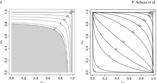
• The fair premium of a stop loss cover with deductible DisE(max{∑dj=1Xj− D,0}). The corresponding functional isΨ(uuu) =max{∑dj=1F
−1
j (uj)−D,0}; see the left-hand side of Figure 1 for a contour plot ofΨfor two Pareto margins.
• Risk measures for an aggregate sumS=∑dj=1Xj, such as value-at-risk, VaRα(S), or expected shortfall, ESα(S), α ∈(0,1), cannot in general be written as an expectation of type E(Ψ0(XXX)). However, they are functionals of the aggre-gate distribution function FS(x) =P(S≤x) =E(Ψ(UUU;x)), whereΨ(uuu;x) = I{F−1
1 (u1)+···+Fd−1(ud)≤x}. We can therefore write
VaRα(S) =inf{x∈R:E(Ψ(UUU;x))≥α}, ESα(S) = 1 1−α
Z 1
α
u1 u2
0.0
0.2
0.4
0.6
0.8
1.0
0.0 0.2 0.4 0.6 0.8 1.0
0.2 1
5 10
20 50
100 200
500 10005000
Fig. 1 Left:Contour lines for the excess functionΨ(u1,u2) =max{F1−1(u1) +F2−1(u2)−10,0},
where the margins are Pareto distributed withF1(x) =1−(1+x/4)−2andF2(x) =1−(1+x/8)−2.
The grey area indicates whereΨis zero.Right:Contour lines for the product functionΨ(u1,u2) = F1−1(u1)F2−1(u2), whereX1∼LN(2,1)andX2∼LN(1,1.5).
allocation methods such as the Euler principle for expected shortfall behave sim-ilarly, see [21] and [15], page 260.
Note that in this framework we follow the convention of [15, Remark 2.1] thatXXX refers to a loss and−XXX to a profit, which is more common in an actuarial context. One could have equally well worked with the profit-and-loss random variable−XXX by changing the area of interest to where components ofXXX are small.
2.1 Archimedean Copulas and Sampling Methods
Archimedean copulas form a popular class of copulas in actuarial science and risk management, as they can capture various types of tail dependence. An Archimedean copula admits the representation
C(u1, . . . ,ud) =ψ(ψ−1(u1) +· · ·+ψ−1(ud)), (4) whereψis a univariate function calledgeneratorand is such thatψ:[0,∞)→[0,1] withψ(0) =1 andψ(∞) =limt→∞ψ(t) =0; alsoψ(t)is continuous and strictly
decreasing on[0,inf{t:ψ(t) =0}]. We review two sampling techniques applicable to Archimedean copulas.
Conditional distribution method
The conditional distribution method (CDM) is a sampling technique that in principle works for any copula. For j∈ {2, . . . ,d}, let
be the conditional distribution of thejth component given the firstj−1 components. As a function ofuj,Cj|1...j−1(uj|u1, . . . ,uj−1)is a univariate distribution function on
[0,1]and thus can be sampled via inversion. Doing this iteratively in jbased on the previously computed component samples leads to a sample fromCaccording to the CDM. The efficiency of this sampling method depends on the computational cost required to evaluate the conditional quantile functionsC−1
j|1...j−1(uj|u1, . . . ,uj−1), which in many cases are not available in closed form. For Archimedean copulas, there exists a more efficient sampling method, which we now describe.
Marshall–Olkin algorithm
It is well established thatψinduces an Archimedean copula for any dimensiond≥2 if and only ifψis the Laplace–Stieltjes transform of a distribution function of some positive random variableV, the so-called frailty. Based onV, one can derive the stochastic representation
ψ
E1
V
, . . . ,ψ
Ed
V
∼C, (5)
where E1, . . . ,Ed ind.
∼Exp(1) are independent of the positive frailty random vari-ableV whose Laplace–Stieltjes transform is ψ. This sampling method is known asMarshall–Olkin (MO) algorithm; see [14].
For many popular Archimedean copulas, the frailty random variableV from the MO algorithm has a known distribution, for instanceV is Gamma distributed for Clayton copulas; see Table 1 for information about five popular Archimedean cop-ulas and the corresponding frailty random variablesV, and see [11, Table 1] for the details concerning Table 1. In Section 4 we develop an IS algorithm that exploits the MO representation of Archimedean copulas.
Family Parameter ψ(t) V
Ali-Mikhail-Haqθ∈[0,1) (1−θ)/(exp(t)−θ) Geo(1−θ)
Clayton θ∈(0,∞) (1+t)−1/θ Γ(1/θ,1)
Frank θ∈(0,∞)−log(1−(1−e−θ)exp(−t))/θ Log(1−e−θ)
Gumbel θ∈[1,∞) exp(−t1/θ) Stable(1/θ,1,cosθ(π/(2θ)),I
{θ=1}; 1)
Joe θ∈[1,∞) 1−(1−exp(−t))1/θ Sibuya(1/θ)
Table 1 Popular Archimedean generators and corresponding frailty distributions.
2.2 Quasi-Monte Carlo and Copula Models
The combination of QMC and copulas is studied in depth in [1]. To describe how it works, letη:[0,1)d+k→[0,1)dfork≥0 be some transformation function such thatη(UUU0)∼CforUUU0∼U[0,1)d+k. The choice ofη corresponds to the choice of sampling methods forC, such as CDM or MO. The plain MC estimator (2) thus becomes
ˆ
µMC,n=
1 n
n
∑
i=1To use QMC, we replace the point set{UUU0i,i=1, . . . ,n}by a low-discrepancy point set. The choice of sampling algorithmη is not very important to control the MC error, but it is for QMC, as explained in [1]. The sampling algorithms we propose in this work are applicable to both MC and QMC, and numerical results for both methods are reported in Section 6. For QMC we use a Sobol’ sequence [20] and ap-ply to it a randomization based on a digital-shift (see [13, Section 6.2.2]) so that we can construct unbiased estimators and compute confidence intervals for the quantity of interest by using replication.
3 Importance Sampling for Copula Models
IS is a popular variance reduction technique for rare event simulations. Suppose we want to estimateE(Ψ(UUU))whereUUU∼C, for ad-dimensional copulaC. In IS, we draw samples from some proposal distribution ˜UUU∼Gand construct the estimator
ˆ µIS,n=
1 n
n
∑
i=1Ψ(UUU˜i)w(UUU˜i), UUU˜i ind.
∼G, (7)
wherew(uuu) = dCdG((uuuuuu)) is the Radon-Nikodym derivative ofCwith respect toG. The functionwworks as a weight function so that the estimator remains unbiased after changing the distribution. Intuitively, the variance of the IS estimator is smaller than the variance of the plain MC estimator if the proposal distribution is concentrated around the important region, which we characterized in Section 2 as the region where the maximal component of a sample point is close to 1.
In order to define the proposal distributionG, we suggest a mixing approach by taking a weighted average of a multivariate distribution functionCλ :[0,1]d→[0,1] over different values ofλ. LetFΛdenote a discrete distribution function of a random variableΛ:Ω 7→[0,1), defined byqk:=P(Λ =λk),k=1, . . . ,M. We then define the distribution functionGof ˜UUUas a mixture ofCλ with respect toFΛ:
G(uuu) =
M
∑
k=1qkCλk(uuu),
whereCλ is a distorted version of the copulaCitself that concentrates samples in a region of the form[0,1]d\[0,λ]d. Note that theC
λ we will construct (see (8)) is a copula only ifC(λ111) =0, butCλ does not need to be copula for our approach to work.
We will see that this mixture approach is natural in order to allowCto be abso-lutely continuous with respect toG. In particular, the absolute continuity is guaran-teed for any copulaCif the following assumption is satisfied.
Assumption 1.The random variableΛ satisfiesP(Λ=0)>0.
In order to obtain a well defined weight functionwand an unbiased estimator ˆ
particular conditions onC. Although it seems restrictive, we will see that it is also needed to have a consistent estimator ˆµIS,n. Moreover, ensuringP(Λ =0)>0 can be seen as a form of defensive mixture sampling, where a fraction of samples are drawn from the original distribution [9]. Defensive sampling bounds the IS weights away from infinity (as will be seen in Lemma 2) so that the resulting estimator has a finite variance. To that end, we assume Assumption 1 to be satisfied in what follows. The construction of the proposal distributionGas aCλ-mixture directly yields a sampling method, as one can draw a realization ofGby first drawingΛ∼FΛ and then ˜UUU∼CΛ. Therefore, the following algorithm can be used to construct ˆµIS,n:
Algorithm 1General IS algorithm for copulas
1: Fixn∈N.
2: DrawΛi∼FΛ,i∈ {1, . . . ,n}.
3: Draw ˜UUUi∼CΛi,i∈ {1, . . . ,n}.
4: Calculatew(UUU˜i) =dC(UUU˜i)/dG(UUU˜i),i∈ {1, . . . ,n}.
5: Return ˆµIS,n=1n∑ni=1Ψ(UUU˜i)w(UUU˜i).
The following lemma establishes consistency and asymptotic normality of the estimator ˆµIS,n.
Lemma 1.Suppose thatVar(Ψ(UUU))<∞and that w(·)≤B for a constant B<∞. Then
1.µISˆ ,nconvergesP-almost surely toµ;
2.σ2=Var(Ψ(UUU˜)w(UUU˜))<∞and√n(µISˆ ,n−µ)→N (0,σ2)in distribution. We will later show that under some mild assumptions onFΛ, the weight function will indeed be bounded on[0,1].
The form ofCλ we propose to work with is the distribution ofUUUconditioned on the event that at least one of its components exceedsλ:
Cλ(uuu) =P(U1≤u1, . . . ,Ud≤ud|max{U1, . . . ,Ud}>λ)
=P(U1≤u1, . . . ,Ud≤ud|UUU∈/[0,λ]d)
=C(uuu)−C(min{u1,λ}, . . . ,min{ud,λ})
1−C(λ111) , (8)
whereλ111=λ(1, . . . ,1) = (λ, . . . ,λ)∈[0,1)d. By putting mass ofΛ on(0,1), we can put more weight on the region of the copula where at least one component is large. For instance, ifFΛis discrete andP(Λ=0) =P(Λ=0.9) =0.5, then 50% of the samples of ˜UUUare constrained to lie only in[0,1]d\[0,0.9]dwhile the other 50% of the samples will lie on[0,1]d. Note that the mass on[0,1]d\[0,0.9]dwould then be higher than 50% since we can still sample from[0,1]d\[0,0.9]dwhenΛ=0. On the other hand, the caseP(Λ=0) =1 yieldsG=CsinceCλ =Cforλ=0.
Theorem 1.The Radon–Nikodym derivative w(uuu) =dC(uuu)/dG(uuu)is given by
w(uuu) =
M
∑
k=1I{λk≤max{u1,...,ud}}
1−C(λk111) qk
−1
.
In order to simplify the notation, letwe:[0,1]→[0,∞)be defined as
e
w(u) =
M
∑
k=1I{λk≤u}
1−C(λk111) qk
−1
. (9)
Therefore we have thatw(uuu) =we(max{u1, . . . ,ud}). In order to evaluatewe, it is
suf-ficient to calculate (or approximate)C(λk111)fork∈ {1, . . . ,M}. These values must be calculated only once and thus this approach is fast and can be easily implemented. In particular, the density ofCdoes not have to be evaluated to calculatew(or ˜w). This is in an advantage in comparison to most other IS algorithms, for which the existence of the density ofCis required.
Lemma 2.Under Assumption 1,w is bounded from above bye P(Λ=0)−1on[0,1]. As a consequence of Lemma 2, Assumption 1 is not only sufficient to obtain existence of the weights, but it also guarantees that they are bounded. In virtue of Lemma 1, this guarantees consistency and asymptotic normality of the IS estimator. Note that our approach could be generalized to other forms ofCλ andFΛ (e.g., not necessarily discrete). In such cases the evaluation of the weight functionwemight be more demanding and require the use of numerical integration schemes.
4 Importance Sampling Algorithm for Archimedean Copulas
While the IS method from the previous section can be applied to any copula, sam-pling fromCλ is in general difficult. A possible solution could be to use rejec-tion sampling, but we do not pursue this approach here as we expect it would not work very well with QMC sampling. In this section, we instead focus on develop-ing sampldevelop-ing algorithms forUUU|U(d):=max{U1, . . . ,Ud}>λ whenUUU follows an Archimedean copula with generatorψ. This corresponds to Step 3 in Algorithm 1. In light of (5), we have (U1, . . . ,Ud)d
= (ψ(E1
V ), . . . ,ψ( Ed
V )) whereEj ind.
∼Exp(1)
andV is the corresponding frailty random variable. The conditionU(d)>λ can then be written as E(1)<ψ−1(λ)V, where E(1)∼Exp(d)is the first order statis-tic of{E1, . . . ,Ed}. In summary, sampling fromUUU|U(d)>λ is equivalent to sam-pling from(E1, . . . ,Ed,V)|E(1)<ψ−1(λ)V. Algorithm 2 summarizes the sampling method for this conditional distribution where we letγ =ψ−1(λ). Proposition 1 asserts that samples from Algorithm 2 have the right distribution.
Algorithm 2Sampling Step of the IS algorithm for Archimedean copulas
Require: 0<γ=ψ−1(λ)<∞.
1: Draw(E(1),V)|(E(1)<γV). 2: Draw(E1, . . . ,Ed)|E(1).
3: LetUj=ψ(Ej/V)forj∈ {1, . . . ,d}.
4: return (U1, . . . ,Ud).
While Proposition 1 holds for general (positive)Ej’s andV, we now give detailed explanations of how to do the sampling for Steps 1 and 2 of Algorithm 2, i.e., when Ej
ind.
∼Exp(1)andV is the frailty random variable. We assume thatV is continuous for the derivations below. We need only minor modifications for the discrete case.
Step 1: Sample(E(1),V)|(E(1)<γV)
We want to sample from the joint distribution of(E(1),V)conditioned on the event (E(1)<γV). Let fE(1)(x)and fV(v)be the density ofE(1) andV, respectively. Fur-ther, let f(E
(1),V)|(E(1)<γV)(x,v) be the conditional joint density of (E(1),V) given
E(1)<γV. Then by independence ofE(1)andV f(E
(1),V)|(E(1)<γV)(x,v) =βfE(1)(x)fV(v)I(x<γv), (10) where 1/β =P(E(1)<γV) =P(U(d) >λ) = (1−C(λ111)) = (1−ψ(dψ−1(λ))). We use conditional sampling to sample from this density, that is, we first sampleV from the marginal conditional density fV|(E(1)<γV) of (10) then drawE(1)from (10) givenV. Note that
fV|(E(1)<γV)(v) =βfV(v) Z γv
0
fE(1)(x)dx=βfV(v)(1−exp(−dγv)). (11)
Unfortunately, the density (11) does not belong to a known parametric family for most Archimedean copulas. Nonetheless, there exist efficient numerical algo-rithms that allow one to sample from a univariate distribution given its probability density function. For instance, the NINIGL Algorithm in [4] achieves this through numerical inversion techniques. Such algorithms could become costly if they had to be applied for several values ofΛ. However in our numerical experiments, the threshold random variableΛ only takes a small number of distinct values, such as 10, which is much less than the number of simulations, which is of order 10,000. Furthermore for each value ofΛ =λ, we sample from (11) thousands of times, which makes the overhead required to initialize the sampling algorithms negligible. After samplingV from (11), we want to drawE(1)givenV. Let the conditional density ofE(1)be denoted by fE
(1)|(E(1)<γV,V)(x|V). Then
fE
(1)|(E(1)<γV)(x|V) =
and we can draw a sample from this density using the inversion technique. In par-ticular, we generateU∼U[0,1)and then letE(1)=−1dlog(1−U(1−e
−γdV)).
Step 2: Sampling(E1, . . . ,Ed)|E(1)
Suppose we have drawnE(1)=x(1)from Step 1. Let f(x1, . . . ,xd) =exp −∑di=1xi
be the joint density of(E1, . . . ,Ed). Note that eachEjis as likely to be the minimum. Consider the case whereE1is the minimum. The conditional distribution is
f(x1, . . . ,xd|E1=E(1),E(1)=x(1)) =
e−x(1)−∑dj=2xj (1/d)de−dx(1) =e
−∑dj=2(xj−x(1))·I
{E1=x(1)}. (12) We can sample from (12) by letting Ej =Exp(1) +x(1) independently for j ∈ {2, . . . ,d}.
Since any of theEj’s can be the minimum, we pick the index for the minimum component randomly from 1 todand sample the rest of the components accordingly. This sampling method works for MC, but may not work very well for QMC. When randomly choosing the index for the minimum component, we potentially destroy the structure of the LDS. So, if we are working with an LDS, the CDM based on Proposition 2 below is preferred.
Proposition 2.Suppose E1, . . . ,Edare iidExp(1). Then
P(Ek≤xk|E1=x1, . . . ,Ek−1=xk−1,E(1)=x)
=
(
1−exp{−(xk−x)}, if xj=x for some j∈ {1, . . . ,k−1}, 1
d−k+1I{xk<x}+
d−k
d−k+1(1−exp{−(xk−x)}), otherwise. (13) To sampleE1, . . . ,Ed, we letktake the successive valuesk∈ {1, . . . ,d}in (13) and proceed by inversion.
4.1 Stratified Sampling Alternative to Importance Sampling
Recall from Algorithm 1 and the form ofCλ given in (8) that our IS scheme starts with sampling a threshold random variableΛ=λkand then proceeds by sampling
˜
UUU∼UUU|(T=max{U1, . . . ,Ud}>λk). Instead, we can construct a stratified sampling (SS) estimator based on the samples fromUUU|(λk+1>T ≥λk). That is, we stratify the domain ofUUUalong withT. SupposeΛ takesMdistinct values as 0=λ1<· · ·< λM<1. LetλM+1=1 for convenience. Then we can defineMstrata as
ˆ
µSS,n=
M
∑
k=1pk nk
nk
∑
i=1Ψ(UUU˜(ik)), (15)
where pk is the stratum probability,nk is the number of samples allocated to the stratumΩk, and ˜UUU
(k) i
ind.
∼UUU|Ωk. For Archimedean copulas,pk=ψ(dψ−1(λk+1))− ψ(dψ−1(λk)). In Section 5, we show that the SS estimator has a smaller variance than the IS estimator. It is easy to show that sampling from Ωk is equivalent to sampling from(E1, . . . ,Ed,V)|ψ−1(λk+1)V<E(1)≤ψ−1(λk)V. Letγk=ψ−1(λk) for allk∈ {1, . . . ,M+1}. Algorithm 3 summarizes the procedure to sample from each stratum.
Algorithm 3SamplingUUUk,jin SS algorithm for Archimedean copulas
Require: 0<γk+1<γk<∞.
1: Draw(E(1),V)|(γk+1V<E(1)≤γkV). 2: Draw(E1, . . . ,Ed)|E(1).
3: LetUj=ψ(Ej/V)forj∈ {1, . . . ,d}.
4: return (U1, . . . ,Ud).
In this algorithm, Step 2 is exactly the same as for the IS case (Algorithm 2). For Step 1, we use conditional sampling to draw samples from the joint conditional density of(E(1),V)|(γk+1V<E(1)≤γkV). By using an argument similar to the one used for Step 1 of Algorithm 2, we can show that the marginal conditional density ofVis
fV|(E(1)<γV)(v) =βfV(v)(exp(−dγk+1v)−exp(−dγkv)), (16)
wherefV(v)is the density ofVandβ=1/pk=1/ψ[dψ−1(λk+1))−ψ(dψ−1(λk)]. Conditional on V drawn from (16), generate U ∼U[0,1) and then let E(1) = −1dloge−γk+1dy−U(e−γk+1dy−e−γkdy). Then(E
(1),V)follows the desired distri-bution.
5 Variance Analysis and Calibration Method
In this section, we analyze the variance of the IS and SS estimators and then propose calibration methods for choosing theqk’s designed to minimize the variance of the respective estimators. We also show that the SS scheme is more flexible to calibrate and gives an estimate with a smaller variance than the IS estimator.
We define the strataΩ1, . . . ,ΩMas in (14) andCk=C(λk111)fork∈ {1, . . . ,M}. The following proposition gives the variance of the IS estimator.
Proposition 3.LetµISˆ ,nbe the IS estimator described in Algorithm 1 with Cλgiven in(8). Then its variance is given by
Var(µISˆ ,n) = 1 n
M
∑
k=1pk k
∑
l=1ql 1−Cl
!−1
µk(2)−µ2
, (17)
where pk=P(UUU∈Ωk), qk=P(Λ =λk)andµk(2)=E(Ψ2(UUU)|Ωk).
For the optimal calibration, we want to choose theqk’s so that (17) is minimized. The following proposition gives an analytical expression for the optimal calibration. For convenience, we defineµ0(2)=0.
Proposition 4.The set of qk’s that minimize(17)under the conditionµ1(2)≤ · · · ≤ µM(2)withµ0(2)=0for convenience, is
qoptk =
(1−Ck)
q
µk(2)−
q
µk(−2)1
M
∑
k=1
(1−Ck)
q
µk(2)−
q
µk(2−)1
, k∈ {1, . . . ,M}. (18)
Remark 2.If the condition µ1(2)≤ · · ·<µM(2) is not met, some of theqoptk ’s given by (18) will be negative, which makes the IS scheme infeasible. Note thatqoptk <0 means that ever having the event[Λ =λk]makes the overall variance greater than when qoptk =0. We propose to then removeλk from the support ofΛ ifqoptk <0. Accordingly, the strataΩk’s will change so the stratum second moments need to be recomputed for the optimal calibration.
Of course, we do not know the true values of theµk(2)’s in practice, so we have to replace them with estimates. As often done for Neyman allocation, we can first run a pilot study with a small number of simulations and estimate theµk(2)’s. The
condi-tionµ1(2)≤ · · ·<µM(2)means that the outer strata must have greater stratum second
incompatible, although there is no guarantee that the former implies the latter. If the ISM is satisfied, then we can substitute (18) into (17) and obtain
Var(µˆISopt,n) =1 n
M
∑
k=1pk
q
µk(2)
!2
−µ2
. (19)
Using the Cauchy-Schwarz inequality, we can show that
VarQ(µˆISopt,n) =1 n
M
∑
k=1pk
q
µk(2)
!2
−µ2
≤
1 n
M
∑
k=1pkµ (2) k −µ
2
!
=Var(µMCˆ ,n).
Equality holds only whenµk(2)is the same for allk. Except for this restrictive case, the IS estimator with the optimal choice ofqk’s always has a smaller variance than the plain MC counterpart. If the ISM is not met, there is no analytical form for the optimalqk’s. We can still find the optimal values using widely available convex optimization solvers in this case. If we letq1=1 andqk=0 fork=2, . . . ,M, the proposal distribution is the same as the original distribution. That is, IS becomes plain MC. Hence, if we choose theqk’s appropriately, the IS estimator cannot do worse than plain MC. In this sense, the IS estimator is similar to an SS estimator.
Now that we have derived the variance expression and the optimal choice ofqk’s, we move on to the stratified sampling estimator (15). Using simple algebra, one can show that Var(µˆSS,n) =∑Mk=1p2kσk2/nk,whereσk2=Var(Ψ(UUU)|Ωk),k∈ {1, . . . ,M} are the stratum variances. The optimalnk’s are given by Neyman allocation
nk=
npkσk
∑Mk=1pkσk
. (20)
Unlike the IS estimator, there is no restriction on this optimal allocation, i.e., we do not needσkto be increasing withk. In this sense, the SS estimator is more flexible. Since the true strata variances are unknown, we have to replace them with esti-mates. Investigating the optimal calibration formula for IS (18) and SS (20), it ap-pears that the estimation error of the strata moments (theµk(2)’s for IS and theσk2’s for SS) has greater impact on the estimated calibration for IS than for SS. Sinceqk for IS depends on
q
µk(2)−
q
µk(−2)1, the estimation error comes from both estimat-ingµk(2−)1andµk(2). On the other hand, for SS,nkdepends onσk, so the estimation error comes from estimatingσk2alone. Consequently, the approximation is likely to deviate more from the actual optimal calibration for IS than for SS.
Proposition 5.Suppose we have an IS estimator withP(Λ=λk) =qk,1≤k≤M. If theµk=E(Ψ(UUU)|Ωk)are not all equal and n is large enough, then there exists some strata sample allocation(n1, . . . ,nM)for the SS estimator such thatVar(µˆSS,n)≤ Var(µˆISdet,n)≤Var(µˆIS,n).
This result trivially holds when we use the optimalqk’s (18) for stratified and un-stratified IS and use the optimal allocation (20) for SS. Since the SS estimator is more flexible for calibration and it has a smaller variance than both IS estimators, the SS approach is preferred if the sampling efforts for (11) and (16) are not sig-nificantly different. Nonetheless, depending on the type of the underlying copula, sampling from the IS distribution could be much easier than sampling from the SS distribution.
6 Numerical Examples
In this section, we investigate the efficiency of the IS and SS estimators introduced in this paper. We consider the valuation of tail-related quantities of a portfolio con-sisting of stocks from companies in the financial industry listed on the S&P 100. The five stocks in the portfolio are AIG, Allstate Corp., American Express Inc., Bank of New York and Citigroup Inc. Their stock symbols are AIG, ALL, AXP, BK and C, respectively. We assume that the value of the portfolio is 100 and that all the portfolio weights are equal. The data are daily negative log-returns of these five companies from 2010-01-01 to 2016-04-01 (1571 data points). We fit GARCH(1,1)-models witht-innovations to each return series to filter out the volatility clustering effect using theRpackage “rugarch” [6]. The fitted standardized residuals do not exactly follow at-distribution, so we fit a semi-parametric distribution to the resid-uals using theRpackage “spd” [7]. The fitted model uses a kernel density estimate for the centre of the distribution and fits a generalized Pareto distribution to the tails. The use of generalized Pareto distribution to model the GARCH filtered residuals to estimate tail-related risk measures in a univariate setting is studied by McNeil and Frey [16]. We letS=∑dj=1Xjdenote the portfolio loss over a one day period with
Xj=100ωj 1− d
∑
j=1exp(aj−bjF˜j−1(Uj))
!
,
whered is the number of assets,ωj’s are the portfolio weights,aj’s are the means of the log-returns, bj’s are the fitted conditional standard deviations from the GARCH(1,1) model, ˜Fj’s are the fitted semi-parametric distributions from theR package “spd”, and(U1, . . . ,Ud)follows the fitted copula. We use theRpackage “distr” [18] to sample from (11) and (16).
The three functionals we estimate are stop lossE(max{S−D,0})withD=3 for Gumbel andD=2 for Frank, VaR0.99 and ES0.99 of S. To defineCΛ, we use λk=1− 12k−1fork=1, . . . ,M, withM=10. When constructing an IS estimator, we stratifyΛ regardless of whether we use MC or QMC. When we calibrate the qk’s for IS according to (18) and SS according to (20), we use ES as our objective function.
Gumbel Frank
MC QMC MC QMC
Objective function d Estimate IS SS Plain IS SS Estimate IS SS Plain IS SS
E(max{S−D,0}) 5 0.012 67 168 33 1730 8085 0.011 6.4 11 14 85 161 20 0.010 49 40 51 1128 3488 0.0034 4.6 4.1 5.7 46 46 VaR0.99(S) 5 3.2 10 26 8.4 39 98 2.4 9.7 9.0 2.6 32 26
20 3.04 7.9 7.2 5.8 19 28 2.1 4.3 4.8 3.6 16 19 ES0.99(S) 5 4.2 89 175 29 6019 16989 2.8 17 21 7.1 250 373
20 4.03 49 39 48 1296 4205 2.3 4.6 3.8 4.0 38 36
Run time 5 3.6 3.7 1.8 3.7 3.8 3.6 3.7 1.1 3.6 3.7 20 2.0 1.9 1.2 1.9 2.0 1.7 1.8 1.1 1.9 2.0
Table 2 Estimates and variance reduction factors for the Gumbel and Frank copulas based on
n=30 000,d=5.
Table 2 shows the estimates, variance reduction factors and computational times for the three functionals for the five different estimators based on Gumbel and Frank copulas, respectively. We used 30 randomizations to estimate the variance of each estimator (MC and QMC). The estimates shown are based on SS estimators with QMC. Variance reduction factors are defined to be the ratios of the variance of the plain MC estimators over the variance of the estimators with the respective VRTs. The last row of Table 2 shows the increase in computation time compared to plain MC. We see that both IS and SS reduce the variance by large amounts and this is amplified when combined with QMC. Note that SS estimators generally give smaller variances than the IS estimators, as suggested by Proposition 5. For IS and SS estimators with and without QMC, we see that the largest variance reduction factors are for ES. This makes sense as we calibrate theqk’s to minimize the variance of the ES estimator.
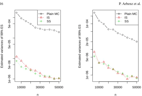
We also repeat the same experiment but with a portfolio of 20 stocks from large companies in the financial industry traded on NYSE (the full list is available from the authors); the results are displayed underd=20 in Table 2. Figures 2 and 3 show the log-variance of the three different MC-based estimators for differentn.
Appendix
Proof of Lemma 1. Since E(Ψ(UUU˜)w(UUU˜)) =E(Ψ(UUU)), consistency follows di-rectly from the Strong Law of Large Numbers. Note that E Ψ(UUU˜)2w(UUU˜)2
=
● ● ● ● ● ● ● ● ● ●
10000 30000 50000
1e−06 5e−06 5e−05 5e−04 n Estimated v ar
iances of 99% ES
● Plain MC
IS SS ● ● ● ● ● ● ● ● ● ●
10000 30000 50000
1e−06 5e−06 2e−05 1e−04 n Estimated v ar
iances of 99% ES
● Plain MC
IS SS
Fig. 2 Estimated variances of plain MC, IS and SIS estimators of ES0.99 for a Gumbel copula
(left-hand side) and a Frank copula (right-hand side) for differentnand ford=5.
● ● ● ● ● ● ● ● ● ●
10000 30000 50000
5e−06 2e−05 1e−04 5e−04 n Estimated v ar
iances of 99% ES
● Plain MC
IS SS ● ● ● ● ● ● ● ● ● ●
10000 30000 50000
1e−06 5e−06 2e−05 5e−05 n Estimated v ar
iances of 99% ES
● Plain MC
IS SS
Fig. 3 Estimated variances of plain MC, IS and SIS estimators of 99% ES for a Gumbel copula
change of measure. We can immediately deduce asymptotic normality of ˆµIS,nby the Central Limit Theorem, see, for example, Section 2.4 in [5], page 110. ut
Proof of Theorem 1.Due to Leibniz’ integral rule,dG(uuu) =R1
0dCλ(uuu)dFΛ(λ). From the definition ofCλ, we can derive the differential
dCλ(uuu) =
(
0, uuu∈[0,λ]d, dC(uuu)
1−C(λ111), otherwise. Using both identities, we obtain
dG(uuu) =dC(uuu) Z 1
0
I{λ≤max{u1,...,ud}}
1−C(λ111) dFΛ
(λ),
leading to the desired result. ut
Proof of Lemma 2.SinceC(λ111),λ ∈[0,1], the diagonal section of the copulaCand the distribution functionFΛ are both increasing functions. The weight functionweis
thus decreasing on[0,1], and is bounded above bywe(0) =P(Λ =0)−1<∞. ut Proof of Proposition 1.We sample(E1, . . . ,Ed,V)|(E(1) <γV)using conditional distribution sampling. That is, we first sample (E(1),V)|(E(1) <γV), which is the Step 1 of Algorithm 2. Given the (E(1),V) drawn, we then want to sample (E1, . . . ,Ed)|(E(1)<γV,E(1),V)which is equivalent to sampling(E1, . . . ,Ed)|E(1)
and this is the Step 2 of the algorithm. ut
Proof of Proposition 2.First, consider the case wherexj=xfor some j=1, . . . ,k− 1. Without loss of generality assume thatx1=x, i.e.,E1=E(1). So we want to find P(Ek ≤xk|E1=x1, . . . ,Ek−1=xk−1,E(1)=E1=x). From (12), the conditional distribution ofEkisx+Exp(1). So the above probability equals
P(Ek≤xk|E1=x1, . . . ,Ek−1=xk−1,E(1)=x) =1−e−(xk−x). (21) Next, we consider the casexj6=xfor all j=1, . . . ,k−1. This means thatEj= E(1)for some j=k, . . . ,d. Since allEjare iid, there is ad−1k+1probability thatEk= E(1). In such a caseEk=xwith probability 1 as we are givenE(1)=x. SupposeEk6= E(1), which occurs with probability ofd−d−k+k1. Then we need to find the probability
P(Ek≤xk|E1=x1, . . . ,Ek−1=xk−1,E(1)=x,Ej6=E(1),j=1, . . .k)
=
d
∑
j=k+11
d−kP(Ek≤xk|E1=x1, . . . ,Ek−1=xk−1,E(1)=x,Ej=E(1))
=P(Ek≤xk|E1=x1, . . . ,Ek−1=xk−1,E(1)=x,Ed=E(1)) =1−e−(xk−x).
The last equality again holds by (12) and the result follows. ut
Proof of Proposition 3.Recall that the IS estimator (7) is
ˆ µIS,n=
1 n
n
∑
i=1Ψ(UUU˜i)w(UUU˜i) = 1 n
n
∑
i=1whereti=max(UUU˜i,1, . . . ,UUU˜i,d), and where the weight function (9) is
e
w(u) =
M
∑
k=1I{λk≤u}
1−Ck qk
−1
. (23)
Hence weis constant over each stratum Ωk. Thus, foruuu∈Ωk, we can define the stratum weight as
wk=
k
∑
l=1ql 1−Cl
−1
, k∈ {1, . . . ,M}. (24)
The second moment ofw(UUU˜)Ψ(UUU˜)is
E(w2(UUU˜)Ψ2(UUU˜)) =E(w(UUU)Ψ2(UUU)) = M
∑
k=1pkE(w(UUU)Ψ2(UUU)|UUU∈Ωk)
=
M
∑
k=1pkwkE(Ψ2(UUU)|UUU∈Ωk) = M
∑
k=1pkwkµ (2) k =
M
∑
k=1pk k
∑
l=11 1−Cl
ql
!−1
µk(2).
The third equality holds because the weight function ˜w(t) is constant over each stratum. The last equality follows from (24). Then the variance of the IS estimator based onnsamples is Var(µISˆ ,n) =1n
∑Mk=1pk
∑kl=11−1Clql −1
µk(2)−µ2
. ut
Proof of Proposition 4.Since the variance expression (17) is convex inqk’s, we can solve the minimization problem using Lagrange multipliers. First, we simplify (17) so that the minimization problem becomes easier. Let ˜pk=P(UUU˜ ∈Ωk), the stratum probability under the proposal distribution. Observe that
˜ pk=
M
∑
l=1ql·P(UUU∈Ωk|Λ =λk) = k
∑
l=1ql·P(UUU∈Ωk|Λ=λk)
=
k
∑
l=1ql·P(UUU∈Ωk|Λ =λk) = k
∑
l=1ql pk 1−Cl
=pk k
∑
l=1ql 1−Cl
. (25)
By (23) and (25), we can writewk=pk/p˜k. The weightwk is the ratio of proba-bilities of a sample falling onto stratumΩkunder the original distribution and the proposal distribution. Plugging this expression into (17), we have
Var(µISˆ ,n) = 1 n
M
∑
k=1p2k ˜ pk
µk(2)−µ2
!
. (26)
Using the Lagrange multiplier method, we can show that the optimal ˜pkis
˜ poptk =pk
q
µk(2)
M
∑
k=1pk
q
Note that this optimal choice of ˜pk’s resembles the Neyman allocation, the optimal allocation under stratified sampling.
Using the relationqk= (1−Ck)
˜ pk
pk−
˜ pk−1
pk−1
, (with ˜p0/p0=0) the optimalqkis
qoptk ∝(1−Ck)
q
µk(2)−
q
µk(−2)1
,(withµ0(2)=0). (28)
The assumption thatµ1(2)≤ · · · ≤µM(2)ensures thatqoptk ≥0 fork=1, . . . ,M. ut Proof of Proposition 5.We have ˆµISdet,n=1n∑Mk=1∑
nqk
j=1Ψ(UUU˜ki)w(UUU˜ki), UUU˜ki iid
∼UUU|Λ=
λk. Thus Var(µˆISdet,n) =E
Var(Ψ(UUU˜)w(UUU˜)|Λ)/n+O(1/n2) (term due to round-ingnqk). Since Var(µISˆ ,n) =1nVar(Ψ(UUU˜)w(UUU˜), we have Var(µˆISdet,n)≤Var(µISˆ ,n)as long asnis large enough for theO(1/n2)term due to rounding to be smaller than Var(E(Ψ(UUU˜)w(UUU˜)|Λ))/n>0. As shown before, ˜pk=P(UUU˜ ∈Ωk) =pk∑kl=1
ql
1−Cl.
Consider an SS estimator with nk =np˜k. Then Var(µSSˆ ,n) = 1n∑Mk=1 p2k
˜ pkσ
2 k. Also Var(Ψ(UUU˜)w(UUU˜)|Λ =λk) =Var(Ψ(UUU˜)w(UUU˜)|T >λk)≥E[Var(Ψ(UUU˜)w(UUU˜)|T > λk,T ∈Ωj)] =∑Mj=k
pj
1−Ckw
2
jσ2j. Then, using (24) andwk=pk/p˜kwe get
Var(µˆISdet,n)≥ 1 n
M
∑
k=1qk M
∑
j=kpj 1−Ckw
2 jσ2j =
1 n
M
∑
k=1pkw2kσk2 k
∑
j=1qj 1−Cj
=1
n M
∑
k=1pkwkσk2=1 n
M
∑
k=1p2k ˜ pk
σk2=Var(µSSˆ ,n).
u t
Acknowledgements We thank the anonymous referees for their helpful comments. The third and
fourth author gratefully acknowledge the financial support of NSERC Canada through grant num-bers #5010 and #238959, respectively.
References
1. Cambou, M., Hofert, M., Lemieux, C.: Quasi-random numbers for copula models. Statistics and Computing27(5), 1307–1329 (2017)
2. Chan, J., Kroese, D.: Efficient estimation of large portfolio loss probabilities in t-copula mod-els. European Journal of Operational Research205(2), 361–367 (2010)
3. Choe, G., Jang, H.: Efficient algorithms for basket default swap pricing with multivariate Archimedean copulas. Insurance: Mathematics and Economics48(2), 205–213 (2011) 4. Derflinger, G., H¨ormann, W., Leydold, J.: Random variate generation by numerical inversion
when only the density is known. ACM Trans. Model. Comput. Simul.20(4), 1–25 (2010) 5. Durrett, R.: Probability: theory and examples, fourth edn. Cambridge Series in Statistical and
Probabilistic Mathematics. Cambridge University Press, Cambridge (2010)
8. Glasserman, P., Li, J.: Importance sampling for portfolio credit risk. Management science
51(11), 1643–1656 (2005)
9. Hesterberg, T.: Weighted average importance sampling and defensive mixture distributions. Technometrics37(2), 185–194 (1995)
10. Hofert, M., Kojadinovic, I., Maechler, M., Yan, J.: copula: Multivariate Dependence with Cop-ulas (2016). R package version 0.999-15
11. Hofert, M., M¨achler, M., et al.: Nested archimedean copulas meet R: The nacopula package. Journal of Statistical Software39(9), 1–20 (2011)
12. Huang, P., Subramanian, D., Xu, J.: An importance sampling method for portfolio cvar estima-tion with gaussian copula models. In: Proceedings of the 2010 Winter Simulaestima-tion Conference (WSC), pp. 2790 – 2800 (2010)
13. Lemieux, C.: Monte Carlo and Quasi-Monte-Carlo Sampling. Springer (2009)
14. Marshall, A., Olkin, I.: Families of multivariate distributions. Journal of the American Statis-tical Association83(403), 834–841 (1988)
15. McNeil, A., Frey, R., Embrechts, P.: Quantitative Risk Management: Concepts, Techniques, Tools. Princeton University Press, Princeton (2005)
16. McNeil, A.J., Frey, R.: Estimation of tail-related risk measures for heteroscedastic financial time series: an extreme value approach. Journal of Empirical Finance7(3), 271–300 (2000) 17. Nelsen, R.: An Introduction to Copulas, second edn. Springer, New York (2006)
18. Ruckdeschel, P., Kohl, M., Stabla, T., Camphausen, F.: S4 classes for distributions. R News
6(2), 2–6 (2006)
19. Sak, H., H¨ormann, W., Leydold, J.: Efficient risk simulations for linear asset portfolios in the t-copula model. European Journal of Operational Research202(3), 802–809 (2010) 20. Sobol, I.: On the distribution of points in a cube and the approximate evaluation of integrals.
USSR Comput. Math. Math. Phys.7(4), 86–112 (1967)