G. Di Gennaro, R.J. van Weeren, M. Hoeft, H. Kang, D. Ryu, L. Rudnick, W. Forman, H.J.A. R¨ottgering,2 M. Br¨uggen,7W.A. Dawson,8 N. Golovich,9 D.N. Hoang,2 H.T. Intema,2 C. Jones,1
R.P. Kraft,1 T.W. Shimwell,2 and A. Stroe10
1Harvard-Smithsonian Center for Astrophysics, 60 Garden Street, Cambridge, MA 02138, USA 2Leiden Observatory, Leiden University, PO Box 9513, 2300 RA Leiden, The Netherlands 3Th¨uringer Landessternwarte, Sternwarte 5, 07778 Tautenburg, Germany
4Department of Earth Sciences, Pusan National University, Busan 46241, Korea 5Department of Physics, School of Natural Sciences, UNIST, Ulsan 44919, Korea
6Minnesota Institute for Astrophysics, University of Minnesota, 116 Church St. S.E., Minneapolis, MN 55455, USA 7Hamburger Sternwarte, Universit¨at Hamburg, Gojenbergsweg 112, 21029 Hamburg, Germany
8Lawrence Livermore National Lab, 7000 East Avenue, Livermore, CA 94550, USA 9University of California, One Shields Avenue, Davis, CA 95616, USA
10European Southern Observatory, Karl-Schwarzschild-Str. 2, 85748, Garching, Germany
(Received March 27, 2018; Accepted July 29, 2018)
ABSTRACT
Despite progress in understanding radio relics, there are still open questions regarding the underlying particle accel-eration mechanisms. In this paper we present deep 1–4 GHz VLA observations of CIZA J2242.8+5301 (z = 0.1921), a double radio relic cluster characterized by small projection on the plane of the sky. Our VLA observations reveal, for the first time, the complex morphology of the diffuse sources and the filamentary structure of the northern relic. We discover new faint diffuse radio emission extending north of the main northern relic. Our Mach number estimates for the northern and southern relics, based on the radio spectral index map obtained using the VLA observations and existing LOFAR and GMRT data, are consistent with previous radio and X-ray studies (MRN= 2.58±0.17 and MRS= 2.10±0.08). However, color-color diagrams and modelings suggest a flatter injection spectral index than the one obtained from the spectral index map, indicating that projection effects might be not entirely negligible. The southern relic consists of five “arms”. Embedded in it, we find a tailed radio galaxy which seems to be connected to the relic. A spectral index flattening, where the radio tail connects to the relic, is also measured. We propose that the southern relic may trace AGN fossil electrons that are re-accelerated at a shock, with an estimated strength of M= 2.4. High-resolution mapping of other tailed radio galaxies also supports a scenario where AGN fossil electrons are revived by the merger event and could be related to the formation of some diffuse cluster radio emission.
Keywords: galaxies: clusters: individual (CIZA J2242.8+5301) – galaxies: clusters: intra-cluster medium – large-scale structure of Universe – radiation mechanisms: non-thermal – diffuse radiation – shock waves
Corresponding author: Gabriella Di Gennaro
Di Gennaro et al.
1. INTRODUCTION
Cluster mergers are the most energetic phenomena in the Universe since the Big Bang, involving kinetic en-ergies of ∼ 1063−1065 erg, released over a time scale of 1–2 Gyr (e.g. Sarazin 2002) depending on the clus-ter’s mass and on the relative velocity of the merging dark matter halos. In a hierarchical cold dark mat-ter (CDM) scenario, these phenomena are the natural way to form rich cluster of galaxies. Cluster mergers produce shock waves and turbulence in the intracluster medium (ICM). It has been proposed that ICM shocks and turbulence can (re-)accelerate cosmic rays (CRs) which then produce diffuse radio synchrotron emitting sources in the presence ofµGauss magnetic fields. These diffuse sources are known asradio halosandradio relics (see Brunetti & Jones 2014; Feretti et al. 2012, for a theoretical and an observational review).
Radio halos are centrally located unpolarized sources with a smooth morphology, roughly following the X-ray emission from the ICM. The currently favored forma-tion scenario for the formaforma-tion of radio halos involves the re-acceleration of pre-existing CR electrons (ener-gies of ∼ MeV, e.g. Brunetti et al. 2001; Petrosian 2001) via magneto-hydrodynamical turbulent motions, induced by a merging event. Moreover, radio halos are characterized by a steep-spectrum (α < −1, with
Sν ∝να, e.g. Brunetti et al. 2008). A correlation be-tween the halo radio power and the cluster X-ray lu-minosity exists (e.g. Cassano et al. 2013), showing that the most X-ray luminous clusters host the most powerful radio halos. Moreover, Cassano et al. (2010) showed a clear correlation between the cluster’s dynamical state, measured from the X-ray surface brightness distribution, and the presence of giant radio halos, providing strong support that mergers play an important role in the for-mation of these sources.
As with the radio halos, radio relics are characterized by a steep spectral index (α≈ −0.8 to −1.5). They are generally elongated sources located in the outskirts of clusters, and they are suggested to trace outwards trav-eling shock fronts, where the ICM and magnetic fields are compressed. (e.g. Ensslin et al. 1998; Finoguenov et al. 2010; van Weeren et al. 2010). As a consequence, the magnetic field is amplified and aligned, producing polarized radio emission. One formation scenario for relics is the diffusive shock acceleration (DSA) mech-anism, similar to what occurs in supernova remnants (e.g. Blandford & Ostriker 1978; Drury 1983; Ensslin et al. 1998). This model involves particles (electrons) that are accelerated from the ICM’s thermal pool into CRs at shocks, while the electrons in the downstream region suffer synchrotron and inverse Compton (IC)
en-ergy losses. A prediction of the DSA model is a relation between the Mach number of the shock and the radio spectral index at the shock location (e.g. Giacintucci et al. 2008). However, recent observations suggest fun-damental problems with the standard DSA model: (1) in a few cases, there are cluster merger shocks without cor-responding radio relics (e.g. the main shock in the Bullet Cluster,Shimwell et al. 2014) (2) sometimes, the spec-tral index derived Mach numbers are significantly higher than those obtained from the X-ray observations (e.g. van Weeren et al. 2016), and (3) some relics require an unrealistic shock acceleration efficiency (for DSA) to ex-plain their observed radio power (e.g.Vazza & Br¨uggen 2014;Botteon et al. 2016). Another formation scenario isshock re-accelerationof relativistic fossil electrons (e.g. Markevitch et al. 2005;Macario et al. 2011;Kang & Ryu 2011; Kang et al. 2012; Bonafede et al. 2014; Shimwell et al. 2015;Kang et al. 2017;van Weeren et al. 2017a). This mechanism addresses the DSA efficiency problem, and implies a direct connection between radio relics and radio galaxies, which are supposed to be the primary sources of fossil plasma.
Radio “phoenices” are another class of relics that are characterized by their steep curved spectra and often complex toroidal morphologies. They are supposed to trace AGN fossil plasma lobes which have been adi-abatically compressed by merger shock waves (Enßlin & Gopal-Krishna 2001; Enßlin & Br¨uggen 2002; de Gasperin et al. 2015).
Relics have a range of sizes and morphologies. So-called double relic systems, with two relics located on diametrically opposite sides of the cluster center (e.g. Rottgering et al. 1997;Bagchi et al. 2006;Venturi et al. 2007; Bonafede et al. 2009; van Weeren et al. 2009; Bonafede et al. 2012; de Gasperin et al. 2014) are an important subclass. Numerical simulations (e.g. van Weeren et al. 2011) suggest that these systems are the result of binary mergers between two-comparable mass clusters (mass ratio of 1:1 or 1:3), with the line connect-ing the two relics representconnect-ing the projected merger axis of the system.
2. CIZA J2242.8+5301
CIZA J2242.8+5301 (hereafter CIZA2242) is a merg-ing galaxy cluster located atz= 0.1921 which was first observed in X-ray by ROSAT (Kocevski et al. 2007). This merging cluster has been well studied across the electromagnetic spectrum, from radio, optical, to X-ray bands (van Weeren et al. 2010;Ogrean et al. 2013;Stroe et al. 2013;Ogrean et al. 2014; Stroe et al. 2014; Aka-matsu et al. 2015; Dawson et al. 2015; Jee et al. 2015; Okabe et al. 2015;Donnert et al. 2016;Stroe et al. 2016; Kierdorf et al. 2017; Rumsey et al. 2017), and it has been used as a textbook example for numerical simu-lations aimed to model the shock physics (van Weeren et al. 2011;Kang et al. 2012;Kang & Ryu 2015; Don-nert et al. 2017;Molnar & Broadhurst 2017;Kang et al. 2017).
In the radio band, CIZA2242 shows the presence of a spectacular double relic, located ∼1.5 Mpc north and south from the cluster center. The northern relic is com-posed of an arc-like structure, ∼2 Mpc long and∼50 kpc wide, which suggests the relic traces a shock prop-agating outward, and which gave the cluster the nick-name of the “Sausage” cluster. The cluster also contains a low surface brightness radio halo (van Weeren et al. 2010; Stroe et al. 2013; Hoang et al. 2017). Numeri-cal simulations performed by van Weeren et al. (2011) suggested that the mass ratio of the colliding clusters is between 1.5:1 and 2.5:1, and that the relics are seen close to edge-on (i.e. |i|.10◦). Donnert et al.(2017) showed that, in the northern shock, the upstream X-ray tem-peratures and radio properties are consistent with each other, and consistent with weak lensing cluster masses. Dawson et al.(2015) found two comparable subcluster masses (16.1+4−3..63×1014 M
and 13.0+4−2..05×1014 M for the northern and southern clusters, respectively). Their data was consistent with the interpretation of a merger occurring on the plane of the sky. The time since core passage was estimated to be about 0.6 Gyr byRumsey et al.(2017).
The cluster has an X-ray luminosity ofL500 = 7.7± 0.1×1044erg s−1in the 0.1–2.4 keV energy band, within a radius of R500 = 1.2 Mpc (Hoang et al. 2017). Sev-eral X-ray surface brightness discontinuities were de-tected withChandraandXMM-NewtonbyOgrean et al.
in the radio band (Mradio
N ∼4.6 and MradioS ∼2.8, for the northern and southern relic respectively,van Weeren et al. 2010;Stroe et al. 2013), recent observations show an agreement between the X-ray and the radio Mach number (Mradio
N = 2.9 +0.10
−0.13Stroe et al. 2014,MradioN = 2.7+0−0..63 Hoang et al. 2017 andMradio
S = 1.9 +0.3 −0.2 Hoang et al. 2017).
The Sausage relic has also been observed at high fre-quencies (&2 GHz), where there is still some debate on the integrated radio spectral shape of the relic. New radio observations (up to 30 GHz) revealed a possi-ble steepening in the integrated radio spectrum from
α ∼ −1.0 to α ∼ −1.6 at ν > 2.5 GHz (Stroe et al. 2016), questioning the single power-law spectrum pre-dicted from the DSA model (Ensslin et al. 1998). Pos-sible explanations involve a non-negligible contribution from the Sunyaev-Zel’dovich (SZ) effect (Basu et al. 2016), the presence of a non-uniform magnetic field in the region (Donnert et al. 2016) and evolving shock and re-acceleration models (Kang & Ryu 2015). Contrary to the interferometric observations, no steepening at high frequencies is revealed by single dish observations ( Kier-dorf et al. 2017) at 4.85 and 8.35 GHz, with the Effels-berg Telescope, nor by the combined single-dish Sardinia Radio Telescope interferometric measurements fromLoi et al. (2017). This result led Loi et al. (2017) to sug-gest that the interferometric observations at very high frequency might lose diffuse flux on large angular scales due to the limitation of the minimum baseline length (although Stroe et al. 2016 did attempt to correct for this effect).
re-Di Gennaro et al.
gion. Moreover, Hoang et al. found that the radio halo power is in agreement with the known correlation be-tween the X-ray luminosity and radio power for giant radio halos, and suggested that the halo traces electrons re-accelerated by turbulence generated by the passing shock wave.
3. OBSERVATIONS AND DATA REDUCTION
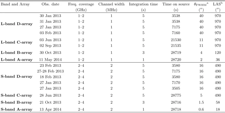
CIZA2242 was observed by the VLA with all the four array configurations in the L- and S-bands, covering the frequency range from 1 to 4 GHz. The total recorded bandwidth was 1 GHz for the L-band, and 2 GHz for the S-bands, split into 16 spectral windows each having 64 channels (1 and 2 MHz width, for the L- and S-band re-spectively). Due to the large angular size of the cluster and the S-band field of view (FOV), we observed three separate pointings. These pointings were located north-west, north-east and south with respect to the cluster’s center. An overview of the frequency bands and obser-vations is given in Table1.
For the primary calibrators we used 3C138 and 3C147, observed ≈5−10 minutes each at the end of the serving run. In some configurations 3C48 was also ob-served (≈8 minutes) near the middle or at the end of the observing run, depending on whether this source was observed in addition to, or in substitution of, the other two primary calibrators. J2202+4216 was included as a secondary calibrator, and observed for ≈3 minutes at intervals of 30-40 minutes. All four polarization prod-ucts (RR, RL, LR and LL) were recorded.
The data were reduced withCASA1 (McMullin et al. 2007) version 4.7.0, and processed in the same way for all the different observing runs. As a first step the data were Hanning smoothed. We removed radio fre-quency interference (RFI) using the tfcrop mode from
theflagdatatask and applied the elevation dependent
gain tables and antenna offsets positions. We deter-mined complex gain solutions for the central 10 chan-nels of each spectral window. In this way we removed possible time variations of the gains during the calibra-tor observations. We pre-applied these solutions to find the delay terms (gaintype=‘K’) and bandpass calibra-tion. Applying the bandpass and delay solutions, we re-determined the complex gain solutions for the primary calibrators using the full bandwidth. We determined the global cross-hand delay solutions (gaintype=‘KCROSS’) from the polarized calibrator 3C138, taking a RL-phase difference of −10◦ (both L- and S-band) and polariza-tion fracpolariza-tions of 7.5% and 10.7% (L- and S-band re-spectively). We used 3C147 to calibrate the
polariza-1https://casa.nrao.edu
tion leakage terms (poltype=‘Df’), and 3C138 to cal-ibrate the polarization angle (poltype=‘Xf’). If not present, we replaced 3C147 with J2355+4950 as polar-ization leakage calibrator. All relevant solutions tables were applied on the fly to determine the complex gain solution for the secondary calibrator J2202+4216 and to obtain its flux density scale. The absolute flux scale from the primary calibrators was calculated assuming the Perley & Butler (2013) model. The RFI removal was repeated after applying the derived calibration so-lutions, using thetfcropmode first and followed by the rflagmode.
All the solutions were transferred to the target source, and then the data were averaged by a factor of two in time and a factor of four in frequency (we excluded the first 7 and the last 10 channels). Finally, a last round of RFI flagging was performed with AOFlagger (Offringa et al. 2010), to remove the remaining interference from the dataset.
To refine the calibration for the target field, we per-formed two rounds of phase-only self-calibration and two of amplitude and phase self-calibration on the individual datasets. The only exceptions were the northeastern and northwestern pointing of the A-array data taken in the S-band, for which the low signal-to-noise ratio (SNR) allowed only for phase-only self-calibration, combining both polarizations (gaintype=‘T’). All imaging inCASA was done with w-projection (Cornwell et al. 2005,2008), which takes the non-coplanar nature of the array into ac-count. We also used briggs weighting (Briggs 1995) with a robust factor of 0. The spectral index was taken into account during the deconvolution, usingnterms=3(Rau & Cornwell 2011). To deconvolve a few bright sources outside the main lobe of the primary beam, image sizes of up to 97202 pixels were needed (in A-array configu-ration). Clean masks were employed during the decon-volution. Initially, the clean masks were automatically made with thePyBDSMsource detection package (Mohan & Rafferty 2015), and then updated after each imaging cycle. We manually flagged some additional data dur-ing the self-calibration process by visually inspectdur-ing the self-calibration solutions.
L-band D-array
27 Jan 2013 1–2 1 5 7175 40 970
03 Feb 2013 1–2 1 5 7160 40 970
L-band C-array 03 Jun 2013 1–2 1 5 21530 11 970
02 Sep 2013 1–2 1 5 21535 11 970
L-band B-array 30 Oct 2013 1–2 1 3 28719 4 120
L-band A-array 11 May 2014 1–2 1 1 28720 2 36
S-band D-array
23 Feb 2013 2–4 2 5 3580 16 490
27-28 Feb 2013 2–4 2 5 7175 16 490
18 Feb 2013 2–4 2 5 3580 16 490
27 Jan 2013 2–4 2 5 7170 16 490
27 Jan 2013 2–4 2 5 3505 16 490
S-band C-array 28 Jun 2013 2–4 2 5 28775 5 490
S-band B-array 21 Oct 2013 2–4 2 3 28716 1.5 58
S-band A-array 13 Apr 2014 2–4 2 1 28718 0.6 18
Note: a synthesized beamwidth;b largest angular scale.
Table 2. Image (CASA) information.
Band Resolution weighting robust uv-taper σrms
(00×00
) (00) (µJy beam−1)
L-band
1.6×1.6 briggs 0 none 5.3 2.5×2.5 uniform N/A 2.5 6.5
6×6 uniform N/A 5 5.8
10×10 uniform N/A 10 8.9
25×25 uniform N/A 25 19
S-band
1.3×1.3 briggs 0 none 3.4 2.5×2.5 uniform N/A 2.5 4.1
6×6 uniform N/A 5 4.5
10×10 uniform N/A 10 5.6
25×25 uniform N/A 25 23
on common uv-distances, discarding all the data below 120λ. The final image resolutions are 1.600and 1.300(full resolution, L- and S-band respectively), and 2.500, 500, 1000 and 2500 (see Table2). We used a multiscaleclean (Cornwell et al. 2008), with scales of [0,3,7,25,60]× the pixel size2 to make these images. The images were
2 We chose the pixel size so that the beam is sampled by≈5 pixels.
Table 3. Image (WSClean) information.
Band Resolution weighting robust uv-taper σrms
(00×00
) (00) (µJy beam−1)
L-band 2.1×1.8 briggs 0 none 3.8 S-band 0.8×0.6 briggs −0.5 none 2.7
LS-band
3.8×3.8 briggs 0 2.5 3.4
6×6 briggs 0 5 4.2
11×11 briggs 0 10 6.2
26×26 briggs 0 25 16.7
corrected for the primary beam attenuation, with the frequency dependence of the beam taken into account
(widebandpbcortask3).
To create a set of “deep” images, we employed thew -Stacking Clean algorithm (WSClean) byOffringa et al. (2014) (Table3). We also stacked images from the L-and S-bL-and data. We only use these images for view-ing purposes and determinations of source morpholo-gies. No flux density measurements or other quanti-tative measurements in this paper have been extracted
Di Gennaro et al.
from them, sinceWSCleanjust provides an averaged flux density across the bandwidth without taking into ac-count the spectral index during the deconvolution.
4. RESULTS
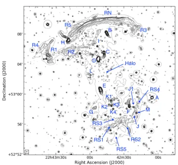
In Figs. 1 and A.1 we present our deep, high-resolution VLA images of CIZA2242, in L- (1–2 GHz, 2.100 ×1.800, weighting briggs’ robust 0 and uniform) and S-band (2–4 GHz, 0.800 ×0.600, weighting briggs’ robust −0.5 and uniform) respectively. The rms noise is 3.8 µJy beam−1 at 1–2 GHz and 2.7 µJy beam−1 at 2–4 GHz (Table3). We also show all the 1–4 GHz lower resolution images produced (Fig. 3). In all the images we detect the two main relics (north and south), and five other areas/regions of diffuse emission and several tailed radio sources above the 3σrms level. We label the cluster sources using the same convention ofStroe et al. (2013) andHoang et al.(2017), see Fig.2.
At full resolution, the length of the northern relic (RN) remains constant between the two frequencies (i.e. ∼1.8 Mpc), while the width decreases from 80 to 40 kpc, in L- and S-band, respectively. The high resolution radio maps show, for the first time, that the relic structure is not continuous, but broken into six different “sheets” or “filaments” (Fig.7) with lengths of about 200−600 kpc. This is visible at both frequencies (Figs. 1 and A.1). The integrated flux densities of RN, measured within the 3σrms region, are 128.1±3.2 mJy and 56.1±1.4 mJy at 1.5 and 3.0 GHz, respectively. We did not included the western emission (R3), for which we measured 12.1±0.3 mJy and 4.5±0.2 mJy, at 1.5 and 3.0 GHz respec-tively4. We also note the presence of additional faint
emission at the 3σrms level located northeastward of the northern relic (4.2±0.2 mJy and 2.1±0.1 mJy, in L-and S-bL-and respectively). We label this emission as R5 (see Fig.2) and, as for R3, it was not included into the RN surface brightness measurement. R5 has an extent of 215 kpc in the full resolution image, but its size in-creases up to 660 kpc in the 1000 resolution image (Fig. 3). On the eastern side, at a distance of about ∼ 30 kpc, a wide-angle tailed source (H in Fig.2) is located, which has a much higher surface brightness than the relic at both frequencies. Comparing the optical and the radio contours of this source (right panel in Fig. 6(d)), we note that the northern lobe breaks ∼50 kpc from the AGN and then proceeds quite straight, while the southern lobe bends immediately, in projection. We also note that the surface brightness of the northern lobe increases by a factor∼4 about 85 kpc northeast of the
4Hoang et al.(2017) measured one single integrated flux value for RN and R3 (1548.2±4.6 mJy at 145 MHz)
host galaxy. The southern lobe, on the other hand, is ∼7 times brighter than the northern one (Flobe S= 21.5 mJy and Flobe N = 3.2 mJy at 1.5 GHz). The zoom on the the northern relic (Fig. 7) shows that the flux boost in the northern lobe coincides with the RN6 fila-ment, while the brighter southern lobe is approximately located along the extent of the RN1 filament.
At a distance of about 600 kpc east of source H, there is another arc-like patch of diffuse emission, labeled R1. This relic extends in the north-south direction for a length of≈610 kpc, while the width changes from about 20 kpc to 100 kpc, going from north to south. The flux density of this diffuse source is about one order of mag-nitude lower than RN: we measure 16.0±0.5 mJy and 7.8±0.3 mJy, at 1.5 and 3.0 GHz respectively. We also note that the southern part of R1 is brighter than the rest of this relic. East of R1, faint emission, labeled as R4, extends for ≈ 315 kpc in NW-SE direction. The size of R4 increases up to 640 kpc, at 1000 resolution. This emission was also detected byHoang et al.(2017), who labeled it as R1 east (and R1 as R1 west). South of RN/H, we detect a patch of extended emission with a toroidal morphology, labeled R2. Although the 3σrms emission is seen only within a region of 180×210 kpc, some residuals cover a broader region, which is better detected at lower resolutions (Fig.3). At 500 resolution, the size increases to 710×250 kpc. Towards the west, we detect source I, which was also reported byStroe et al. (2013) and Hoang et al. (2017). It is barely detected in our high-resolution images, but it is clearly visible in our low resolution images (Fig. 3). Our images reveal that source I is a≈825 kpc long filament that connects with R2.
At full resolution, the southern relic (RS) is well detected only in the L-band image. It is located ≈ 2.5 Mpc south of RN, and formed by two “arms”, la-beled RS1 and RS2 in Fig.2. They measure 530×70 and 25×380 kpc, respectively. We measure a total flux density for these two “arms” of 16.7±0.5 mJy and 7.7±0.3 mJy, at 1.5 and 3.0 GHz respectively. More-over, at lower resolutions we also detect three additional “arms”, labeled RS3, RS4 and RS5, extending eastwards and westwards (Fig.2). The southern relic has a total size of≈1.5 Mpc at 2500 resolution.
H
R1 R4
R5
R3 B
C D
E
F
J
RS G
R2
I
K2 K1
K3
K4
Figure 1. L-band (1.5 GHz) VLA high-resolution image of CIZA2242. The map has a noise ofσrms= 3.8µJy beam−1. The black arrows highlight the “broken” nature of the radio tails. Sources are labeled followingStroe et al.(2013) andHoang et al.
(2017) (see Fig. 2for a more complete labeling).
mJy, at 1.5 and 3.0 GHz respectively. Moreover, at low-resolution source J seems to be completely embedded into the southern relic (bottom right panel in Fig.3).
Towards the north of RS, the patchy extended emis-sion detected by Stroe et al. (2013) and Hoang et al. (2017) is now resolved into four different sources, which are now labeled in Fig.2as K1 (tailed radio source), K2, K3 and K4 (compact radio sources). All these sources have and optical counterpart (see Fig. A.2and the zoom in right panel in Fig. 6(g)). A patch of diffuse emission
is detected on the east of these radio galaxies, namely source G. No clear optical counterpart has been found to be associated to this source from previous optical stud-ies (Dawson et al. 2015, Fig. A.2and the zoom in right panel in Fig. 6(f)).
Di Gennaro et al.
RN
RS1 R1
R4
R2
R3
A B
C
D
E
F G
H I
J K1
R5
K2 K3 J1 L
RS2 RS4
RS3
RS5 Halo
M K4
Figure 2. Labeled cluster sources, adapting the scheme from Stroe et al.(2013) andHoang et al.(2017). We used the 500 resolution (black solid line) to emphasize the diffuse emission. The grey solid line is the 3σradio contour at 2500 resolution. The radio contours are the same of the ones in Fig.3).
16.7 µJy beam−1) level at 2500resolution (bottom right panel in Fig.3). It extends the entire distance between RN and RS, with a size of about 2.1 Mpc×0.8 Mpc (N-S and E-W directions, respectively), at this resolu-tion. To estimate the halo radio flux density, we need to remove the contribution of radio galaxies and other sources. This is not trivial, since some these sources are also characterized by some extended emission.
To construct a model for the emission of the extended and compact sources (e.g. radio galaxies, R2 and source I), we imaged the data with the same settings as for the 500 resolution image (uniform weighting and a uv-taper of 500), since it catches properly the diffuse emission from the tails. To avoid the emission of the halo, we include an inner uv-cut of 0.86kλ, which filters out the emission scales larger than 40 (∼ 770 kpc at cluster’s redshift). The model of the radio galaxies was then subtracted from the uv data by means of the task uvsub. Finally, the new visibilities were re-imaged at low resolution (i.e. a uv-taper of 3500 and uniform weighting) and the final image was primary-beam corrected.
The measured halo radio flux density at 1.4 GHz is 25.2±4.1 mJy. This flux density measurement agrees with the previous result found by Hoang et al.(2017).
The flux density results in a 1.4 GHz radio power5 of P1.5 GHz = (2.69±0.37)×1024 W Hz−1. The total error on the halo flux density has been estimated in-cluding the flux scale uncertainty (i.e. 2.5%), image noise (i.e. σ3500 = 36.3 µJy beam−1) scaled to halo
area, and the uncertainty due to the subtraction of the discrete radio sources in the same region (σsub, see Eq. 1 in Cassano et al. 2013). We used σsub = 2.5% of the total flux of the subtracted radio galaxies, given by the ratio of the post-source subtraction residuals to the pre-source subtraction flux of a nearby compact source (RA = 22h41m33s.02 and DEC = +53◦1100500.63, J2000). Additional uncertainties come from the estima-tion of the halo size and from the flux recovered during the imaging (Bonafede et al. 2017). Therefore, we con-sider this value a lower limit. Unfortunately, the LAS (largest angular scale) of the halo does not allow us to properly recover all the halo flux at 3.0 GHz, hence we do not report a flux density measurement at this fre-quency.
Table 4. Flux densities and integrated spectral index of the diffuse cluster sources measured from the full resolution VLA images.
Source S1.5 GHz S3.0 GHz αint
(mJy) (mJy)
RN 128.1±3.2 56.1±1.4 −1.19±0.05
RS 16.7±0.5 7.7±0.3 −1.12±0.07
R1 16.0±0.5 7.8±0.3 −1.03±0.06
R2 10.3±0.4 4.5±0.2 −1.19±0.09
R3 12.1±0.3 4.3±0.2 −1.43±0.07
R4 4.0±0.2 2.3±0.1 −0.93±0.11
R5 4.2±0.2 2.1±0.1 −0.93±0.12
I 3.4±0.2 1.5±0.2 −1.18±0.17
Halo 25.2±4.1 . . . .
A study of the tailed radio galaxies was performed in detail by Stroe et al. (2013). Similar to this previ-ous work, we find that the majority of the radio tails are stretched in the north-south direction, tracing the merger direction. Interestingly, our deep high-resolution images reveal that source C and F have “broken” tails
5 P
1.4 GHz = 4πD2LS1.4 GHz(1 +z)−(α+1) W Hz−1, where
DL= 944 Mpc is the luminosity distance and (1 +z)−(α+1)the
Figure 3. Combined L- and S-band (1–4 GHz) VLA deep images at low resolution (2.500, top left; 500, top right; 1000, bottom left; 2500, bottom right). The beam size is displayed in the bottom left corner of each image. The radio contours are at 3σrms×
p
[1,4,16,64, . . .], where σ2.500 = 3.4µJy beam−1, σ500 = 4.2 µJy beam−1, σ1000 = 6.2µJy beam−1, σ2500 =
16.7µJy beam−1.
(see black arrows in Fig. 1 and A.1), although they are located at different places in the cluster. In con-trast with the previous classification as a head-tail radio galaxy (Stroe et al. 2013), our highest resolution images reveal that source B is a double-lobe source, but where some emission from the lobes has been stripped back-wards in the north-south direction, suggesting possible stripping of lobe plasma related to the merger event. We also underline the proximity between this tailed ra-dio galaxy and source I (Figs. 2 and 3), although no direct connection is visible in our images. Classical ra-dio tail shapes are seen in sources E and K1, with a tail
extension of 160 and 48 kpc, respectively, based on our 1.5 GHz image. The integrated flux densities of the dif-fuse sources at 1.5 and 3.0 GHz6 and the spectral index between these two frequencies, are reported in Table4. All the spectral index values are in agreement with pre-vious works, i.e. Stroe et al. (2013) and Hoang et al. (2017). We estimated the spectral index uncertainties
Di Gennaro et al.
by taking into account the map noise (σrms) and a flux scale uncertainty of 2.5%, using:
σα= 1 lnS1.5 GHz
S3.0 GHz
s
∆S1.5 GHz S1.5 GHz
2
+
∆S3.0 GHz S3.0 GHz
2
(1)
where ∆Sν =
q σ2 rms Asource Abeam
+ (0.025×Sν)2 is the
to-tal uncertainty onSν, while Asource andAbeam are the area of the source and beam respectively.
4.1. Spectral index maps
We combine our 1–2 and 2–4 GHz VLA images with previous observations performed at 610 (van Weeren et al. 2010) and 145 MHz (Hoang et al. 2017) to ob-tain spectral index maps over a wide frequency range. To take into account the differences of each dataset (e.g. interferometer uv-coverage), we produced new radio im-ages for the previous datasets, cutting at a common uv-distance (120λ). We used uniform weighting to com-pensate for differences in the uv-plane sampling. The images of each dataset were then convolved to the same resolution, and re-gridded to the same pixel grid (i.e. the LOFAR image). The effective final resolutions and the noise levels are listed in Table2.
We obtained the spectral index maps by fitting both first and second order polynomials through the flux mea-surements. Although the maximum signal to noise ratio (SNR) is given by the former case, the latter one allows us to take into account possible non-negligible deviation from a straight spectrum. We proceeded as follow:
1. fit with a second order polynomial;
2. determine if the spectral index shows significant curvature (i.e. above the 2×σ threshold, withσ
the uncertainty associated with the second order term);
3. if the second order term is consistent with zero, we redo the fit and use a first order polynomial; otherwise we keep the second order result.
For the spectral index maps, we accepted theαvalues only when the associated uncertainty was above a given threshold, i.e. σα = 0.2 andσα= 0.4, for the first and second order polynomial fits respectively. In this way we prevent a noisy measurement at a certain frequency from rejecting a possible good fit.
For a first order polynomial fit (i.e. y =a0+a1x), the spectral indexαis defined as the slope of the fit, i.e.
α=a1, while the spectral curvatureC is defined as:
C=−αν1
ν2+α
ν2
ν3 (2)
where ν1 is the lowest of the three frequencies, ν2 the middle one and ν3 the highest, as described by Leahy & Roger (1998). In this convention, the curvature is negative for a convex spectrum. Since this curvature definition works only when we have three frequencies, we define the curvature C in the following way (Stroe et al. 2013):
C=αhigh−αlow (3)
where, in our case, the low frequency spectral index was calculated using the LOFAR and the GMRT observa-tions, and the high low frequency spectral index was calculated using the L- and S-band VLA observations. The uncertainty associated with this measure is:
σC=
q
(σαlow)
2+ (σ αhigh)
2 (4)
where the spectral index uncertainties σαlow and σαhigh
were obtained similarly to Eq. 1.
When the second order polynomial fit (i.e. y=a0+ a1x+a2x2) was used, we defined the curvature,C, and the spectral index,α, as
C=a2 (5)
α= dy
dx x
≡ν=608 MHz
=a1+ 2a2x , (6)
respectively. By using this convention, convex spectra are characterized by more negative values of C. The uncertainties associated with α and C were obtained via Monte Carlo simulation.
The spectral index maps at 1000 and 2500of the entire cluster are shown in Figs.4and5, respectively. The cor-responding spectral index uncertainty map at 1000 reso-lution is presented in Fig.B.2.
22h42m00s
30s
43m00s
30s
44m00s
Right Ascension (J2000)
+52°52'
56'
+53°00'
04'
08'
Declination (J2000)
Figure 4. 1000spectral index map of CIZA2242 obtained between 145 MHz, 610 MHz, 1.5 GHz, and 3.0 GHz. The radio contours are from the LOFAR image, with contours drawn at levels of 3σrms×
p
[1,4,16,64,256, . . .], withσrms= 230µJy beam−1. The most important cluster sources have been labeled as Fig. 2.
All the radio galaxies show a spectral index gradient, as expected from cluster galaxies, with a steepening from
α≈ −0.6 in the nuclei toα≈ −2.0 in the tails (sources E and K1, left panel in Figs. 6(c) and (g), respectively). An exception is source B, where the spectral index gra-dient (α∼2) is seen in the south-west direction and not along the nucleus-lobe axis (left panel in Fig. 6(a)), sup-porting a scenario of plasma stripping as consequence of the cluster merger. A remarkable steep gradient is de-tected in sources F and J (left panel in Fig. 6(e)), the spectral index reaching values lower than−2.5. More-over, for the first time we detect spectral index values across the region connecting J1 (α ≈ −0.6) and the
lobe of source J, with values of about−1.6 (left panel Fig. B.1). Particularly interesting is source H, where the spectral index has a gradient (from α ≈ −0.6 to
α≈ −1.9) only in the southern lobe, while it remains quite constant in the northern lobe (fromα≈ −0.6 to
spec-Di Gennaro et al.
22h42m00s 30s
43m00s 30s
44m00s
Right Ascension (J2000)
+52°52' 56' +53°00' 04' 08' 12'
Declination (J2000)
2.0 1.8 1.6 1.4spectral index1.2 1.0 0.8 0.6
22h42m00s 30s
43m00s 30s
44m00s
Right Ascension (J2000)
+52°52' 56' +53°00' 04' 08' 12'
Declination (J2000)
0.04 0.06 0.08spectral index uncertainty0.10 0.12 0.14 0.16 0.18 0.20
Figure 5. 2500spectral index (left panel) and spectral index uncertainty (right panel) maps of CIZA2242 obtained between 145 MHz, 610 MHz, 1.5 GHz, and 3.0 GHz. The radio contours are from the LOFAR image, contours are drawn at levels of 3σrms×
p
[1,4,16,64,256, . . .], withσrms= 340µJy beam−1.
troscopic confirmation has been found so far (Dawson et al. 2015, Fig. A.2).
We made use of the 2500 resolution images (Fig. 5) to determine the spectral properties of the radio halo, which are consistent with the ones obtained by Hoang et al. (2017). No gradient is seen across the halo, and the spectral indices range between −1.2 and−1.0.
5. DISCUSSION
The Sausage cluster is a well known double-relic sys-tem. Due to its size, regularity, and radio brightness, it offers a unique opportunity to study the particle (re-)acceleration mechanisms at shocks, and the parti-cle aging in the shock downstream region, with a rel-atively small contribution from projection effects. In-deed, numerical simulation byvan Weeren et al. (2011) has shown that CIZA2242 is a binary cluster merger seen very close to edge-on (i.e. |i| .10). Here we dis-cuss the relics’ morphologies, formation scenarios, and underlying particle (re-)acceleration mechanisms.
5.1. Radio Mach number estimates
For the DSA model, there is a relation between the radio injection spectral indexαinjand the Mach number M of the shock (e.g. Drury 1983; Blandford & Eichler 1987):
M=
s
2αinj+ 3 2αinj−1
. (7)
One usually assumes a standard power-law energy dis-tribution of relativistic electrons just after acceleration7.
For “stationary conditions”, with the lifetime of the shock and the electron diffusion time being much longer than the electron cooling time, the integrated spectral indexαintis steeper than the injection index by 0.5 ( Kar-dashev 1962):
αinj= 0.5 +αint. (8)
However, the assumption that the timescale on which the shock properties change is much longer than the elec-tron cooling time does not necessarily have to hold for relics (Kang 2015). For example, for a spherically ex-panding shock, Kang established that the slow decline of the injected particle flux over time could increase the low frequency radio emission downstream away from the shock. This means thatαinjcalculated by Eq.8can lead to significant errors in the derived Mach number (i.e. 0.2 units inα).
Therefore, a more accurate way to compute the Mach number from the radio spectral index, would be to di-rectly measureαinjat the shock front and not useαint. At the shock front, where the particles have recently been (re-)accelerated, the injection spectral index should be “flat”, while it should steepen in the downstream re-gion because of synchrotron and IC energy losses. How-ever, directly measuringαinj, requires (i) highly-resolved maps of the downstream cooling region, to avoid the
7 dN(E)
dE ∝E
(a) source B (b) sources D (bottom left) and C (top right)
(c) source E
break
peak
(d) source H
(e) sources F (top left) and J (bottom right) (f) source G
K1
K2
K3
K4
(g) sources K1 (top), K2 (left), K3 (right) and K4 (bottom)
Figure 6. Tailed radio galaxies in CIZA2242 (for the labels see Fig.3). Left panels: 500resolution spectral index map with the 1–4 GHz radio contours at the same resolution. Right panels: Subarugri composite optical images (Dawson et al. 2015; Jee et al. 2015) with the 0.800×0.600(cyan) 2–4 GHz, and 2.500(white) and 500(red) 1–4 GHz radio contours. For both panels, the radio contours are drawn at 3σ×p
Di Gennaro et al.
mixing of different electron populations and (ii) mini-mum projection effects, which means that the merger should have to occur in, or close to, the plane of the sky. Numerical simulations (e.g.van Weeren et al. 2011; Kang et al. 2012) have indicated that for CIZA2242 the projection effects are probably small, at least for the northern relic, with a merger axis angle|i|.10◦. Fur-thermore, the mixing of emission from regions with dif-ferent spectral ages can be largely avoided thanks to our high-resolution images, as described in Sect. 4.1.
5.2. Spectral index profiles and color-color diagrams
To investigate possible differences in the spectral in-dex properties at the shock and the energy losses in the post-shock region, we analyzed the spectral index pro-file across the radio relics. We extracted flux densities across the width of the relics in narrow annuli spaced by the beam size. To avoid mixing of emission from regions with different amounts of aging, we used the highest res-olution images available for all frequencies, i.e. 500. The flux densities were fitted with a first order polynomial. Following van Weeren et al.(2012), we did not include the calibration uncertainties (15% on SLOFAR, 5% on SGMRT and 2.5% onSVLA) in the estimation of the flux density uncertainties, as this would shift measurements in different annuli/regions in the same way.
Another way to investigate the spectral shapes is by means of so-called color-color (cc) diagrams (Katz-Stone et al. 1993;Rudnick & Katz-Stone 1996;Rudnick 2001). These diagrams emphasize spectral curvature, since they represent a comparison between spectral indices calcu-lated at low- and high-frequency ranges. In our case, we plotα610MHz150MHzon thex-axis andα13..0GHz5GHz on they-axis (see bottom panel in Fig. 9). Moreover, cc-diagrams are particularly useful to discriminate between differ-ent theoretical synchrotron spectral models, and to give constraints on the injection spectrum.
The time evolution of the CR electron energy distri-bution depends on two parameters:
dE
dt =−(εsync+εIC)E
2, (9)
where εIC is the contribution of the IC energy losses, (i.e. εIC ∝ BCMB2 , where BCMB = 3.25(1 +z)2 µG), while εsync is the contribution of the synchrotron en-ergy losses, whose parametrization depends on the ag-ing model assumed. Generally, a JP (Jaffe & Perola 1973) aging model is used, which involves a single burst of particle acceleration, and a continues isotropization of the angle between the magnetic field and the electron velocity vectors (the so-called pitch angle) on a
time-scale shorter than the radiative timetime-scale8. Here, the
synchrotron losses are described by the εsync ∝ B2 re-lation. Other models include continuous particle accel-eration (CI;Pacholczyk 1970) or a modification to the JP model with a finite period of electron acceleration (KGJP;Komissarov & Gubanov 1994).
One characteristic that makes cc-diagrams particu-larly useful is that the shape of the different models only depends on the injection spectral index, while it is independent of the magnetic field value, adiabatic com-pression/expansion and radiation losses.
5.3. Northern Relic
Our high-resolution images reveal that the northern relic contains filamentary substructures. We labeled these sheets as RN1, RN2, RN3, RN4, RN5 and RN6 in Fig. 7. To avoid mixing of different electron popu-lations, we obtained the spectral index profiles in sev-eral sub-sectors (RN1–RN5). We define each sector such that it does not include regions where two sheets over-lap, or contain compact sources. Despite their different locations, RN1 to RN5 display similarαinjvalues at the shock, and similar trends in the downstream region (see Table5).
The injection spectral index for the RN was estimated by considering a narrow region (with a width identical to the beam-size, i.e. the combined red boxes in Fig.8, bottom panel) following the length of the relic. From this region, we obtainαinj =−0.86±0.05, correspond-ing to a Mach number of MN = 2.58±0.17 (Eq. 7). The injection spectral indices of the different filaments in the northern relic, and the corresponding Mach num-bers, are reported in Table5. We find a good agreement with the X-ray Mach number estimate (MN = 2.7+0−0..74 Akamatsu et al. 2015) and with the previous radio stud-ies (MN = 2.9+0−0..1013, Stroe et al. 2014; MN = 2.7+0−0..63, Hoang et al. 2017).
To investigate possible variations across the length of RN, we calculated the spectral index in individual beam-sized regions at the shock front (red boxes in Fig. 8 bottom panel). The results are shown in the top panel in Fig.8and suggest that the eastern part (.1 Mpc) of RN is slightly steeper than the western one. However, given the uncertainties on the spectral indices of the two relic sides, i.e. αinj,.1Mpc = −0.89±0.05 and αinj,&1Mpc = −0.81±0.08, this difference is not significant. Significant spectral index variation are visible on smaller scales (i.e. ∼ 200 kpc): we measure a flattening of the spectral index around 1600 kpc, and a steepening around 400
Figure 7. Full resolution (2.100×1.800) L-band image zooming in the northern relic. The black arrows indicate the points where the relic breaks into several separate sheets.
Table 5. Spectral indices and Mach numbers for the relics in CIZA2242. A comparison with literature values is shown in columns 5, 6 (radio) and 7 (X-ray).
Region res. αinj Mradio? Mradio† Mradio‡ MX−ray
(00)
RN 5 −0.86±0.05 2.58±0.17 2.9+0.10 −0.13 2.7
+0.6 −0.3 2.7
+0.7 −0.4 RN1 5 −0.89±0.05 2.47±0.14
RN2 5 −0.90±0.03 2.46±0.07
RN3 5 −0.89±0.04 2.47±0.10
RN4 5 −0.81±0.04 2.72±0.16
RN5 5 −0.89±0.10 2.48±0.38
RN6 5 −0.84±0.16 2.62±0.86
RS 10 −1.09±0.05 2.10±0.08 2.8+0.19∗∗ −0.19 1.9
+0.3∗∗ −0.2 1.7
+0.4 −0.3 R1 10 −0.82±0.02 2.69±0.06 2.4+0.5
−0.3 2.5 +0.6‡ −0.2 R4 10 −0.86±0.04 2.57±0.12
R5* 10 −1.06±0.21 2.13±0.55
Note: ?this work;† Stroe et al.(2014,2013), for the north and south relics, respectively; ‡Hoang et al.(2017); Aka-matsu et al.(2015). * Source is only visible in our new deep VLA images, hence we calculated the spectral index (and de-rived the Mach numbers) only between 1.5 and 3.0 GHz flux density measurements. ** Obtained at different resolutions: 1800Stroe et al.(2013) and 2500(Hoang et al. 2017).
and 1000 kpc (see Fig. 8). Mach number variations, or different aging trends with the broken-shaped shock surfaces, different amounts of mixing, and magnetic field variation are possible explanations (see Sect.5.3.3).
5.3.1. Spectral curvature
In Fig. 9 we display the spectral index and the cur-vature profiles, and the color-color diagram for the RN4 filament (see the bottom panel of Fig. 8 for the sector placement), obtained with a first order polynomial fit. The steepening of the spectral index in the post-shock region (top panel in Fig. 9) qualitatively agrees with synchrotron and IC energy losses. The non-negligible curvature in each annulus, which was also detected by Stroe et al. (2013), is better seen in the middle panel in Fig. 9, where the curvature profile is shown. All the points in the plot lie below the C = 0 line, and the convexity of the spectrum (C <0, see Eq. 3) increases further towards the cluster center. In the cc-diagram we also show the JP and KGJP (solid and dash-dotted lines, respectively) aging models. Theα610MHz
Di Gennaro et al.
RN1 RN2
RN3
RN4 RN5
Figure 8. Top panel: East-west spectral index profile (blue circles) obtained with a first order polynomial fit and VLA flux densities at 1.5 and 3.0 GHz (orange and green squares, respectively) at 500-resolution of the northern relic. The filled red region represents the standard deviation associated with the injection spectral index (red solid line). Bottom panel: 1–4 GHz 500resolution image of the northern relic. The red boxes shown the beam-sized region where the spectral in-dices were extracted. The yellow sectors represent the re-gions where we extracted the spectral index and curvature profiles and the color-color diagram.
a surprise since the northern relic is almost 2 Mpc long and it is likely that it is also characterized by extended emission in the third dimension. This would easily led to regions with slightly different amounts of spectral aging being contained in a single annulus. Moreover, we note that this effect is stronger further downstream towards the cluster center. A similar result has also been seen for the Toothbrush cluster (van Weeren et al. 2012). We describe the effects of the projection in Sect. 5.3.2.
Interestingly, the injection spectral index directly ob-tained from the spectral index map is slightly different from the one obtained via the cc-diagram (αinj,2Dmap ≈ −0.8 while αinj,model = −0.7). The first point in our color-color diagram, at the relic’s outer edge, already shows a small amount of spectral curvature indicating that even at this location there is already some mixing of emission with different spectral ages, likely due to pro-jection effects. Extrapolation in the cc-diagram to the
αlow=αhighline might therefore provide a more reliable estimate than simply taking the flattest spectral index
5.3.2. 3D model
When computing the spectral model in Section5.3.1, it was assumed that the relic is caused by a planar shock front perfectly aligned with the line of sight. The actual shock front in a merging cluster, which causes a radio relic, has certainly a much more complex geometry. A better approximation, although still very simplistic, is the assumption that the shock front is shaped like a spherical cap with uniform Mach number.
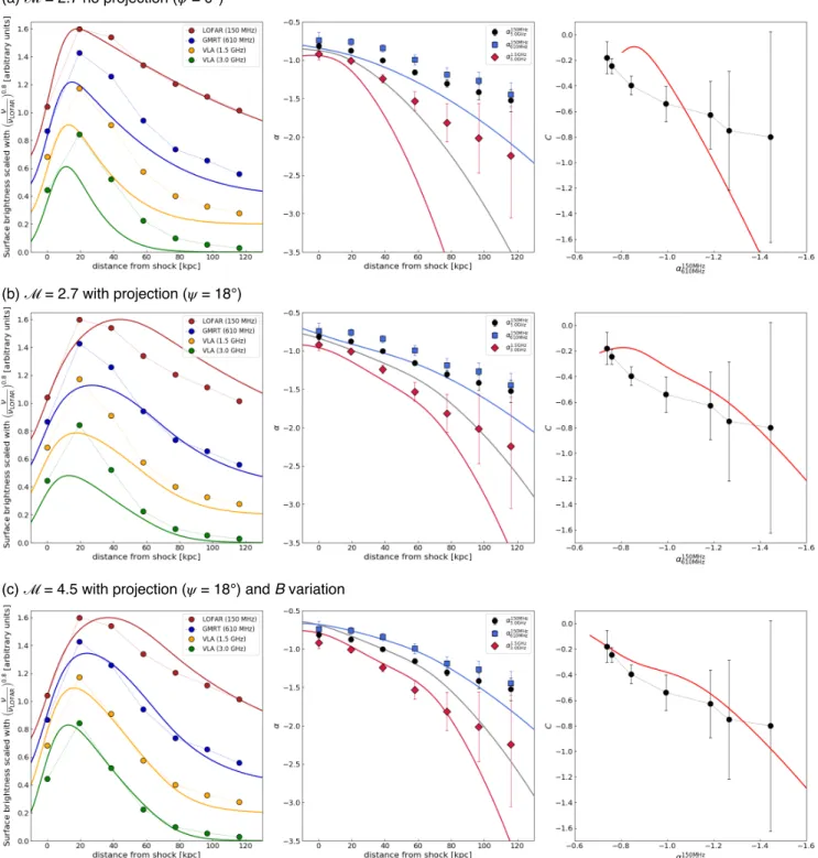
Before we assess the spherically-shaped shock front, we model the profile of a plane shock, i.e. without including any projection effects. We compute the ra-dio emission in the downstream region as described by Hoeft & Br¨uggen (2007). The model assumes a power-law spectrum for the electron energy distribution at the location of injection. A proper average over pitch an-gles was recently included (Hoeft et al. in prep.) to best represent the fast electron velocity isotropization according to the JP model. The resulting model profiles are convolved with the observation resolution, i.e. 500. The top row in Figure10shows the profiles for our four observing frequencies (left panel), and the spectral in-dex (central panel) and curvature (right panel) profiles assuming a shock aligned with the line of sight (ψ= 0◦), a Mach number ofM= 2.7 (i.e. αint =−0.82) accord-ing to the X-ray analysis (seeAkamatsu et al. 2015) and spectral index profile (see Tab. 5), and a homogeneous magnetic field of B = 3 µG. As a result, the peak of the flux density profiles is shifted towards to the down-stream region of the shock, even though the injection is located at the rising flank of the profiles. Although the flux profile at 150 MHz is matched well, this model fails to describe the profiles at the other frequencies, result-ing in a much steeper spectral index profile with respect to that observed (central top panel in Fig. 10).
A possible fix might be made by introducing projec-tion effects, which mix the emission coming from the outermost region and what appears to be in the down-stream region in the 2D plane. To create a toy model, we adopt a curvature radius of the shock of R = 1.5 Mpc and an opening angle of 2ψ = 36◦. This implies that, in projection, there is injection up to about 60 kpc in the downstream direction. The middle row in Figure 10shows the resulting profiles. Evidently, the flux pro-files (left panel) get wider and the spectral index profile
assess the implications, we adopt a quite flat injection index, namelyαinj=−0.6 (M= 4.5)9. Moreover, as it has been pointed out for the “Toothbrush” cluster ( Ra-jpurohit et al. 2018), since we expect that the magnetic field is not homogeneous for a projected Mpc-size shock front, we also included a log-normal distribution for the magnetic field B in the downstream region (see Eq. 7 in Rajpurohit et al. 2018). The best match of our ob-served and modeled profiles is given by a magnetic field strength of B0 = 1 µG and scatter logσ = 1.0. The resulting profiles are shown in the bottom row in Figure 10. The flux densities now match reasonably well and the shapes of the profiles are similar to the observed ones. Although, there are still clear deviations for dis-tances larger than 80 kpc. The discrepancy between the toy model and the observed profiles might be attributed to a much more complex shape of the shock front, injec-tion spectral index and efficiency variainjec-tions across the shock front, and a more complex magnetic field distri-bution including large scale modes. However, our study, combined with the recent results by Rajpurohit et al. (2018) on the “Toothbrush” relic, seems to support the importance of the combination of projection effects and magnetic field variation in the downstream region to ex-plain the cooling of the electrons.
5.3.3. Origin of the filaments
The existence of filaments/sheets in the northern relic is not completely unexpected, since numerical simu-lations show that shock surfaces are complex-shaped structures (e.g.Vazza et al. 2012;Skillman et al. 2013) and the shock Mach numbers are not constant. In com-bination with a highly non-linear shock acceleration ef-ficiency (e.g. Hoeft & Br¨uggen 2007) this would lead to morphologically complex radio relics, with the radio emission primarily tracing localized regions with higher Mach numbers.
Another possibility is that the sheets trace magnetic structures. If they are produced by strands of strong magnetic fields this would imply strong magnetic fields with coherence lengths of Mpc in cluster outskirts. This
9 Such choice comes from Eq. 8, whereα
Di Gennaro et al.
(a) ℳ = 2.7 no projection (𝜓 = 0°)
(b) ℳ = 2.7 with projection (𝜓 = 18°)
(c) ℳ = 4.5 with projection (𝜓 = 18°) and B variation
S2 =
B2
, (10)
where α is, in our case, the injection spectral index, −0.86 (see Tab. 5). According to Eq.10, to explain a flux variation of ∼ 55% (i.e. between the flux density peak at ∼ 1600 kpc and the plateau between ∼1100– 1400 kpc10, i.e. S
2≈0.22 andS1≈0.1 mJy at 1.4 GHz, see top panel in Fig. 8), we need a magnetic field vari-ation of about 30%. The possible influence of the mag-netic field on the radio emission can be addressed via po-larization measurements. A Faraday Rotation Measure analysis for CIZA2242 will be presented in an upcoming paper.
Another possibility to generate non-uniform radio emission is in the re-acceleration scenario. In this case, brightness variations might reflect initial variations in the distribution of fossil radio plasma. A non-uniform distribution of fossil plasma is to be expected consider-ing the complex morphologies of tailed radio galaxies in clusters.
Observational evidences of filaments in radio relics have been found in instances, for example in A 2256 (Owen et al. 2014) and in 1RXS J0603.3+4214 (i.e. the “Toothbrush” cluster,Rajpurohit et al. 2018). However, with the current data in hand we cannot distinguish be-tween the various scenarios above. It is also possible that the sheet-like, filamentary morphology is due to a combination of two or more effects.
5.4. Southern Relic
Our low-resolution images (> 1000) show that the southern relic has a complex morphology. Unlike RN, which is characterized by a single arc-like shape at low resolution, this relic is formed by five “arms” (see Fig.2). This complex morphology does not allow us to produce a clear spectral index profile. Thus, we only calculated the radio Mach number from the injection spectral in-dex, following the same procedure as carried out for RN, avoiding the compact sources. We did that at 1000 reso-lution, a compromise between resolution and SNR. We follow the relic from RS1 to RS4, including the lobe
10The flux density peak at∼1600 kpc is located in the RN4 filament, while the plateau partly covers both RN3 and RN4. We chose these regions because they represent the strongest flux vari-ation.
RS1 RS2
RS3
RS4
RS5
Figure 11. East-west spectral index profile (blue circles) obtained with a first order polynomial fit and VLA flux den-sities at 1.5 and 3.0 GHz (orange and green squares, respec-tively) at 1000-resolution of the southern relic. The filled red region represents the standard deviation associated with the injection spectral index (red solid line). Bottom panel: 1– 4 GHz 1000resolution image of the southern relic. The red boxes shown the beam-sized region where the spectral indices were extracted.
coinci-Di Gennaro et al.
Figure 12. Color-color diagram of the southern region of CIZA2242, using the flux densities extracted in 1000×1000 boxes as shown in the inset in the bottom right corner (same images as the bottom panel in Fig. 11). Red squares are obtained from the area covered by the RS1, RS2 and RS4 “arms” of the southern relic. The black dots come from the lobe of source J. The yellow diamonds represent the values obtained from the radial binning (yellow annuli in the inset).
dent with the location of source J. Around 400 kpc, we measure the steepest spectral index values, coincident with the end of the tail of source J (see Fig.5).
X-ray observations performed withSuzaku(Akamatsu et al. 2015) found a Mach number for RS of 1.7+0−0..45. Al-though this value is comparable within the uncertainties to our radio spectral index derived Mach number, the injection spectral index is affected by the presence of the embedded source J, which is characterized by a very steep spectral index (see Fig. 5). The actual injection spectral index might thus be somewhat flatter.
The spectral index map shows a spectral index steep-ening from the relic outskirts towards the cluster center (Fig. B.1). To investigate whether this region is char-acterized by curved spectra, like RN, we created a cc-diagram using the flux densities extracted in 1000×1000 boxes (i.e. the beam size) covering RS1, RS2, RS4 and the lobe of source J (see the red and black boxes, respec-tively, in the inset in the bottom right corner in Fig. 12). To keep the values with the best SNR, we selected only flux densities above a threshold of 4σrms,ν(whereσrms,ν the noise of each radio map, see Tab. 2). Moreover, we also created a cc-diagram dividing the RS1 “arm” in 1000-wide annuli (yellow sector in the same inset). In-terestingly, we found that all the values for the RS1, RS2 and RS4 regions (red squares in Fig. 12), as well
as the radial distribution (yellow diamonds in the same Figure), fall along the α610MHz
150MHz = α31..5GHz0GHz line. This is somewhat surprising result as curved spectra would be expected due to aging. These results suggest that that (i) at each location, there is an actual power law which represents the steady-state solution to the local shock strength, and that shock strength varies through-out the region, or (ii) there is at each location a very broad range of magnetic fields and/or electron loss his-tories which smear out the underlying spectra, and make them close to power-law. It remains an open question, though, why different power laws at different locations are present for this relic.
5.5. A case for fossil plasma re-acceleration?
There are several issues with the DSA model for ra-dio relics. For some relics, the required fraction of en-ergy flux through the shock surface that needs to be transfered to CR electrons to explain the observed ra-dio power is too large (e.g.Vazza & Br¨uggen 2014;van Weeren et al. 2016). The absence of relic emission at some shocks (e.g. Shimwell et al. 2014) is also puz-zling. In addition, in a few cases, discrepancies have been found between the Mach numbers measured from X-ray observations and those calculated from the ra-dio spectral index (e.g. van Weeren et al. 2016). The re-acceleration of fossil electrons would address some of these problems.
CIZA2242 represents an interesting case to study the interplay between the diffuse radio emission and the tailed radio galaxies. We propose that Source J, which is completely embedded in the southern relic RS, presents a possible case of shock re-acceleration because: (i) there is a morphological connection between the tailed radio galaxy, source J, and the relic. We find that source J consists of an active radio core (J1) and a single jet that ends up in a lobe-like structure (right panel in Fig.6(e)); (ii) A Suzaku analysis revealed the presence of a tem-perature jump roughly at the location of RS (Akamatsu et al. 2015); finally, (iii) the spectral index map dis-plays a steepening from the radio core (J1) through the radio lobe and then a flattening at the cluster shock (right panel in Fig. 6(e)). Also, the cc-diagram for the lobe of source J (black dots in Fig. 12) shows values both on and below the α610MHz
150MHz =α 3.0GHz
Figure 13. Left panel: 1–4 GHz 500resolution image of source J. We overlay the 500(gray) and 2.500(black) resolution radio contours, at 3σand 3σ×p
(1,4,16, . . .), respectively. Right panel: Spectral index profile at 608 MHz, derived by a second order polynomial fit (Eq. 6), across source J obtained from the red boxes in the left panel. The yellow and green squares trace the VLA L- (1.5 GHz) and S-band (3.0 GHz) flux densities across the radio tail, respectively.
and “moved” towards the power law line. Such flatten-ing has been observed recently in the Abell 3411-3412 system (van Weeren et al. 2017a), MACS J0717.5+3745 (van Weeren et al. 2017b) and Abell 1033 (de Gasperin et al. 2017).
5.5.1. Modeling the spectral index change with re-acceleration
FollowingKang et al.(2017), we attempt to model the observed spectral index change from the lobe of source J to the relic RS11. We assume a region of fossil plasma
that is run over up by a spherically expanding shock propagating through the cluster outskirts. To obtain the spectral index distribution across the relic, we extract the flux densities at 500 resolution, following the shape of the tail (left panel in Fig.13). We consider an energy spectrum of the fossil electrons following a power-law distribution with exponential cutoff, of the type:
f(γe)∝γe−sexp
−
γ
e
γe,c
2
, (11)
where s= 1−2αis the injection index from the AGN and γe,c the cutoff Lorentz factor. We use a typical AGN injection spectral index, i.e. α = −0.75 (e.g. Mullin et al. 2008), corresponding tos= 2.5. The spec-tral index where the tail meets the relic (box 13), i.e.
11SeeKang & Ryu(2015) for the geometry of the cloud con-taining the fossil electrons.
α=−2.4 at 608 MHz (right panel in Fig. 13), gives a cutoff Lorentz factor of γe,c = 4.2×10³. This param-eter mimics the steepening of the fossil plasma along the radio tail, and is expected to change with distance from the AGN. We set the post-shock temperature to 9.0±0.6 keV, based on theSuzakudata (Akamatsu et al. 2015), and assume an “extension angle” ofψ= 12◦(van Weeren et al. 2017a). We also included post-shock tur-bulent re-acceleration withτ0= 108 yrs (for details see Kang et al. 2017), which prevent the faster steepening behind the shock (purple dotted line in the top panel of Fig. 14). The pre-shock magnetic field was assumed to be 2.2µG, similar to the magnetic field in the lobes of radio galaxies, leading to a post-shock value of 4.9µG.
The post-shock profile of the radio spectral index de-pends mainly on the shock Mach number and the mag-netic field strength (top panel Fig. 14). Our best-fit model reproduces the spectral change from box 13 (i.e. just before the re-acceleration) to box 19 (i.e. immedi-ately after re-acceleration behind the shock) by assum-ing a sonic Mach number of Ms = 2.4, corresponding to a pre-shock temperature of 3.4 keV12. Such Mach number is chosen to match the radio spectral index
α608 MHz ≈ −0.9 at the relic edge (box 19 in Fig. 13). This value is not consistent with the Suzaku analysis (i.e. M= 1.7+0−0..43andTpre= 5.1+1−1..52keV, respectively),
12 Tpost
Tpre =
5M4+14M2−3
Di Gennaro et al.
Figure 14. Top panel: Spectral index profile calculated at 608 MHz with a second order polynomial fit (Eq.6) from the shock position to the region just before the re-acceleration (boxes from 19 to 13 in the left panel in Fig. 13). Bot-tom panel: Volume-integrated spectrum of the shock region, obtained by assuming a constant pre-shock electron density distribution. Lines display models for different pre- and post-shock magnetic fields as indicated in the legend of the figures.
although the Mach number in the latter case could be underestimated because of instrumental limitations. It is also true, though, that since the fossil electrons are expected to cool due to Coulomb and synchrotron/IC losses advecting away from the AGN core, assuming a constant value forγe,c is a simplification. However,γe,c would not change significantly over∼100kpcscales, i.e. the length of the re-acceleration region, since the radia-tive cooling time scale for electrons with γ <4.2×10³ is tcool > 2.2×10⁸ yr, which is much longer than the shock crossing time (i.e. ≈6.7×10⁷ yr). Additionally, it has been shown that changes in theγe,c value do not affect significantly the energy spectrum of post-shock electrons, since the re-acceleration process “erases” most of the spectral information from the seed fossil parti-cles (see also Supplementary Figure 10 in van Weeren
et al. 2017a). Last but not least, the complex radio tail morphology with a superposition of electron popu-lations could also be the reason of the Mradio/MX−ray discrepancy.
For the re-acceleration, the radio flux density profile across the relic’s width and the integrated spectrum also depend on the spatial variation of fossil electrons. Gen-erally, the radio emission is expected to be the brightest at the approximate shock location, while it fades down-stream of the shock because of energy losses. Instead, we find an opposite trend, with the highest fluxes decreas-ing towards the shock front (see left panel Fig.13, from box 13 to 19). However, the model can reproduce rea-sonably well the observed volume-integrated spectrum (red solid line in the bottom panel of Fig.14). Likely, the shock downstream region is “contaminated” by ra-dio plasma from the lobe of source J, which is embedded in the relic. The failure to accurately predict the flux profiles in the shock downstream region highlights the difficulties of modeling complex AGN lobe emission and its interactions with a shock, in addition to particle re-acceleration in the same general region.
5.6. The relation between tailed radio galaxies and diffuse cluster sources
As discussed above, RS, or at least part of RS, seems to be related to the tailed radio source J. However, this could not be the unique case in CIZA2242, which con-tains a number of complex shaped relics (R1, R2, I, R3, and RS) and tailed radio sources (sources C, D, F, and H). In this section, we speculate that some of the other diffuse relics are also related to AGN fossil plasma that has been revived, either by re-acceleration or solely by adiabatic compression.
a relic (J, RS), patch of fossil plasma (G), and large Mpc-sized complex shaped diffuse sources (RS, R2-I). Whether fossil plasma and re-acceleration are required to produce the main northern relic remains an open question though. Despite the fact the formation scenario for the northern relic remains unclear, our observations do imply that to produce realistic models of diffuse clus-ter radio emission, fossil plasma will need to be included in simulations.
6. CONCLUSIONS
We have presented deep 1–4 GHz VLA observations of the galaxy cluster CIZA J2242.8+5301 (z = 0.1921). This cluster is one of the best examples of a merging system, hosting two Mpc-size relics and several other diffuse radio sources. Our images reached a resolu-tion of 2.100×1.800 and 0.800×0.600 and a noise level of 3.8µJy beam−1and 2.7µJy beam−1at 1.5 and 3.0 GHz respectively. These observations were combined with ex-isting GMRT 610 MHz and LOFAR 150 MHz data (van Weeren et al. 2010;Stroe et al. 2013;Hoang et al. 2017) to carry out a radio continuum and spectral study of the cluster. The main results of our study are summarized below:
• The high-resolution images reveal that the north-ern relic (RN) is not a continuous structure, but is broken up into several filaments with a length of ∼ 200−600 kpc each. Moreover, we detect and characterize additional radio emission north of RN, labeled as R5.
• In agreement with previous studies, we find a trend of North-South spectral steepening for the north-ern relic, indicative of IC and synchrotron energy losses in the downstream region of a shock. We measure an injection spectral index at the shock front from the radio map of −0.86±0.05, corre-sponding to a Mach number of M= 2.58±0.17. Although this value is consistent with the Mach number estimated from X-ray studies, a color-color diagram shows a small amount of spectral curvature at the relic’s northern edge indicating mixing of emission with different spectral ages, possibly due to projection effects. This suggests
it might be partly explained by the presence of AGN fossil plasma that has been revived by the passage of a shock wave. Interestingly, the color-color diagram revealed no curvature in the down-stream region of the southern relic, which can be explained either by a sum of power-law spectra with different αinj at different locations or smear-ing of broad range of magnetic fields and/or elec-tron loss histories.
• We identify source J, a tailed radio galaxy embed-ded in RS, as possible source of fossil radio plasma. Our spectral index maps suggest that old plasma from the lobe of source J is re-accelerated. We attempted to model the flattening of the spectral index from the lobe to the relic RS. We find that a M= 2.4 is compatible with the observed spectral index change.
• The cluster contains several tailed radio galaxies, which show disturbed morphologies likely due to the interaction between the radio plasma, ICM, and the merger event. In addition, the cluster contains a number of complex diffuse radio sources that seem to be related to plasma from tailed radio sources (source G, RS, I, R2). The range in mor-phologies of tailed-radio sources, strong signs of interactions with the ICM, and presence of nearby complex-shaped relics suggest that fossil plasma from cluster radio galaxies plays an important role in the formation of (at least some) diffuse radio sources. To produce realistic models of diffuse cluster radio emission, this fossil plasma will need to be included in simulations.