Data mining scenarios for the discovery of subtypes and the comparison of algorithms

Da

t

a

M

ining Scenarios

f

o

r

t

he

Di

scove

r

y o

f

S

ub

t

ypes and

Da

t

a

M

ining Scenarios

f

o

r

t

he

Di

scove

r

y o

f

S

ub

t

ypes

and

t

he

C

o

m

pa

r

i

son o

f

Al

go

r

it

h

m

s

PROEFSCHRIFT

ter verkrijging van

de graad van Doctor aan de Universiteit Leiden,

op gezag van Rector Magnificus Prof. mr. P. F. van der Heijden,

volgens besluit van het College voor Promoties

te verdedigen op woensdag 4 maart 2009

te klokke 13.45 uur

door Fabrice Pierre Robert Colas

Dr. Ingrid Meulenbelt, LUMC

Prof. dr. F. Famili, NRC-IIT, Ottawa, Canada Prof. dr. T.H.W. B¨ack, LIACS, Universiteit Leiden Prof. dr. G. Rozenberg, LIACS, Universiteit Leiden Prof. dr. B.R. Katzy, LIACS, Universiteit Leiden

This work was carried out under a grant from the Netherlands BioInformatics Center (NBIC).

Data Mining Scenarios for the Discovery of Subtypes and the Comparison of Algorithms

Fabrice Pierre Robert Colas Thesis Universiteit Leiden

ISBN 978-90-9023888-3

Copyright c_!2008 by Fabrice Pierre Robert Colas

All rights reserved. No part of the material protected by this copyright notice may be reproduced or utilized in any form or by any means, electronic or mechanical, including photocopying, recording or by any information storage and retrieval system, without the prior permission of the author.

Printed in France

I

n

t

r

odu

c

t

i

on

Data mining scenarios . . . 1

Part I: Subtype Discovery by Cluster Analysis . . . 1

Part II: Automatic Text Classification . . . 3

Publications . . . 5

Part I: Subtype Discovery by Cluster Analysis . . . 5

Part II: Automatic Text Classification . . . 6

I

Sub

t

ype

D

i

scove

r

y by

C

l

us

t

e

r

A

na

l

ys

i

s

9

1

A

pp

li

ca

t

i

on Do

m

a

i

ns

1.2 Osteoarthritis . . . 11

1.3 Parkinson’s disease . . . 14

1.4 Drug discovery . . . 17

1.5 Concluding remarks . . . 19

2

A

S

ce

n

a

r

i

o

f

o

r

Sub

t

yp

e

D

i

s

c

ov

e

r

y by

C

l

us

t

e

r

A

n

a

l

ys

i

s

2.2 Data preparation and clustering . . . 22

2.2.1 Data preparation . . . 22

2.2.2 The reliability and validity of a cluster result . . . 23

2.2.3 Clustering by a mixture of Gaussians . . . 26

2.3 Model selection . . . 27

2.3.2 Valid model selection . . . 27

2.4 Characterizing, comparing and evaluating cluster results . . . 28

2.4.1 Visualizing subtypes . . . 28

2.4.2 Statistical characterization and comparison of subtypes . . 29

2.4.3 Statistical evaluation of subtypes . . . 31

2.5 Concluding remarks . . . 34

3

R

e

li

a

b

ili

t

y o

f

C

l

us

t

e

r

R

e

su

l

t

s

f

o

r

D

iff

e

r

e

n

t

T

im

e

A

d

j

us

t

m

e

n

t

s

3.2 Methods . . . 36

3.3 Experimental results . . . 38

3.4 Why does optimizing ther2 not boost the clusterreliability? . . . 40

3.5 Concluding remarks . . . 41

4

Sub

t

yp

i

ng

i

n

O

s

t

e

o

a

r

t

h

r

i

t

i

s

,

P

a

r

k

i

nson

’

s d

i

s

ea

s

e a

nd D

r

ug D

i

s

c

ov

e

r

y

4.2 Subtyping in Osteoarthritis . . . 44

4.2.1 Outline of the analysis . . . 44

4.2.2 Model selection . . . 45

4.2.3 Subtype characteristics and evaluation . . . 46

4.3 Subtyping in Parkinson’s disease . . . 48

4.3.1 Outline of the analysis . . . 49

4.3.2 Model selection . . . 49

4.3.3 Subtype characteristics . . . 50

4.3.4 Outline of thepost hoc-analysis . . . 50

4.4 Subtyping in drug discovery . . . 52

4.4.1 Outline of the analysis . . . 53

4.4.2 Model selection . . . 53

4.4.3 Subtype characteristics . . . 55

4.5 Concluding remarks . . . 59

5

S

ce

n

a

r

i

o

I

m

p

l

e

m

e

n

t

a

t

i

on

a

s

t

h

e

R SubtypeDiscovery

P

acka

g

e

5.2 Design of the scenario implementation . . . 62

5.2.1 Methods for data preparation and data specific settings . . 63

5.2.2 The dataset class (cdata) and its generic methods . . . 64

5.2.3 The cluster result class (cresult) and its generic methods 65 5.2.4 Statistical methods to characterize, compare and evaluate subtypes . . . 67

5.2.5 Other methods . . . 68

5.3 Sample analyses . . . 68

5.3.2 Analysis on the principal components . . . 69

5.4 Concluding remarks . . . 70

II

A

u

t

o

m

a

t

i

c Te

x

t

C

l

ass

i

fi

ca

t

i

on

73

6

A

S

ce

n

a

r

i

o

f

o

r

t

h

e

C

o

m

p

a

r

i

son o

f

A

l

go

r

i

t

h

m

s

i

n

Te

x

t

C

l

a

ss

ifi

ca

t

i

on

6.2 Conductingfair classifier comparisons . . . 76

6.3 Classification algorithms . . . 77

6.3.1 kNearest Neighbors. . . 78

6.3.2 Naive Bayes . . . 78

6.3.3 Support Vector Machines . . . 78

6.3.4 Implementation of the algorithms . . . 82

6.4 Definition of the scenario . . . 82

6.4.1 Evaluation methodology and measures . . . 82

6.4.2 Dimensions of experimentation . . . 83

6.5 Experimental data . . . 85

6.5.1 To study the behaviors of the classifiers . . . 86

6.5.2 To study the scale-up of SVM in large bag of words feature spaces . . . 86

6.6 Concluding remarks . . . 87

7

C

o

m

p

a

r

i

son o

f

C

l

a

ss

ifi

e

r

s

7.2 Experimental data . . . 90

7.3 Parameter optimization . . . 90

7.3.1 Support Vector Machines . . . 90

7.3.2 kNearest Neighbors . . . 92

7.4 Comparisons for increasing document and feature sizes . . . 94

7.5 Related work . . . 97

7.6 Concluding remarks . . . 97

8

Do

e

s S

V

M

S

ca

l

e

up

t

o

L

a

r

g

e

B

a

g o

f

W

o

r

ds

F

ea

t

u

r

e

Sp

ace

s

?

8.2 Experimental data . . . 100

8.3 Best performing SVM . . . 100

8.4 Nature of SVM solutions . . . 101

8.5 A performance drop for SVM . . . 104

8.6 Relating the performance drop tooutliers in the data . . . 106

8.8 Concluding remarks . . . 108

C

onc

l

us

i

ons

110

Subtype Discovery by Cluster Analysis . . . 113 Automatic Text Classification . . . 115

A

ppend

i

ces

118

A

T

w

o D

im

e

ns

i

on

a

l

M

o

l

ec

u

l

a

r

D

e

s

c

r

i

p

t

o

r

s

B A

dd

i

t

i

on

a

l

R

e

su

l

t

s

i

n

Te

x

t

C

l

a

ss

ifi

ca

t

i

on

B

i

b

li

og

r

a

phy

S

a

m

e

nv

a

tt

i

ng

C

u

rr

i

c

u

l

u

m

V

i

t

ae

The wordmethodology comes from the latinmethodus andlogia. It is defined by

the Longman dictionary as a body of methods and rules employed by a science

or a discipline [lon84]. It is defined by the Tr´esor de la Langue Fran¸caise asun

ensemble de r`egles et de d´emarches adopt´ees pour conduire une recherche[cnr85].

The work presented in this thesis contributes to the field ofdata mining in

its methodological aspects. This means that we also consider what is needed in

applications besides the selection of algorithms.

The outline of the rest of this introduction is as follows. We start by

introduc-ing the concept ofdata mining scenarios which underlies our two contributions.

Then, we set the context for our firstscenariothat searches for homogeneous

sub-types of complex diseases like Osteoarthritis (OA) and Parkinson’s disease (PD),

and it is also used to identify molecule subtypes in the field of drug discovery.

Next, we introduce our secondscenariofor thecomparison of algorithms in text

classification. Finally, in this introduction, we relate the content of the chapters with our publications.

Da

t

a

m

i

n

i

ng scena

r

i

os

Ascenariois defined by the Longman as(an account or synopsis of) a projected,

planned, anticipated course of action or events.

Therefore, we define a data mining scenario as a logical sequence of data

mining steps to infer patterns from data. Ascenariowill involve the data

prepa-ration methods, it will model the data for patterns, it will validate the patterns and assess their reliability.

In this thesis, we present two data mining scenarios: one forsubtype discovery

P

a

r

t

I

:

Sub

t

ype

D

i

scove

r

y by

Cl

us

t

e

r

A

na

l

ys

i

s

For diseases like Osteoarthritis (OA) and Parkinson’s disease (PD), we are

inter-ested to identifyhomogeneous subtypes by cluster analysisbecause it may provide

a more sensitive classification and hence contribute to the search for the under-lying disease mechanism; we do so by searching for subtypes in values of markers that reflect the severity of the diseases.

In drug discovery, subtype discovery of chemical databases may help to un-derstand the relationship between bioactivity classes of molecules, thus improving our understanding of the similarity (and distance) between drug- and chemical-induced phenotypic effects.

To this aim, we developed adata mining scenario forsubtype discovery (see

Figure 1 for an overview) and we implemented it as theR SubtypeDiscovery

pack-age. This scenario facilitates and enhances the task of discovering subtypes in data. It features various data preparation techniques, an approach that repeats data modeling in order to select for the number of subtypes and/or the type of model, along with a selection of methods to characterize, compare and evaluate statistically the most likely models.

!"#"$%&'%"&"#()*

!"#$%&"'()*+#%&,# !"-.#/',+01/% !",1/%'2$-'#$1, !"!2#&/$,3

+,-.#'&$"*",/.(.

!"%1(&2"4'+&("52*+#&/$,3

0)!',$.','+#()*

!"/&6&'#&("52*+#&/"%1(&2$,3 !"789"+51/&"','2:+$+

.-1#/%'$+2"&"+#'&(3"#()*$ "*!$+)0%"&(.)*

!"3/'6;$5"5;'/'5#&/$-'#$1, !"+#'#$+#$5'2"5;'/'5#&/$-'#$1, !"+#'#$+#$5'2"51%6'/$+1, !"+*4#:6&"/&6/1(*5$4$2$#:

.-1#/%'$.#"#(.#(+",$ '4",-"#()*

!"<=>?"2'%4('"+$4+ !"<=>?"311(,&++"10"!#"#&+# !"<(/*3"($+51@&/:?"9;$A"%'/3$,'2+

In Chapter 1, we describe the background of the current three applications. In Chapter 2, we discuss the different steps of our subtyping scenario. We motivate our choice for a particular clustering approach and we present additional methods that help us to select, characterize, compare and evaluate cluster results. Additionally, we discuss some issues that occur when preparing the data.

Chapter 3 investigates two key elements when searching for subtypes. First, when preparing the data, because age in OA and disease duration in PD are known

to contribute largely to the variability,how to deal with the time dimension? And

second, as we aim for reliable subtypes exhibiting robustness to little changes in

the data,how to assess the reliability of the results?

In Chapter 4, we report subtyping results in OA and PD, as well as in drug discovery. Because of the confidentiality issues regarding the clinical data and the drug discovery data, only a subset of the results is presented.

Finally, Chapter 5 describes the implementation as the R SubtypeDiscovery

package of ourscenario. By making it available as a package, it can be used in

the search for subtypes in other application areas.

P

a

r

t

II

:

A

u

t

o

m

a

ti

c Te

x

t

Cl

ass

i

fi

ca

ti

on

In text categorization, we can use machine learning techniques to build systems which are able to automatically classify documents into categories. For this

pur-pose, the most often used feature space is thebag of words feature space where

each dimension corresponds to the number of occurrences of the words in a doc-ument. This feature space is particularly popular because of its rather simple implementation and because of its wide use in the field of information retrieval.

Yet, the task of classifying text documents into categories is difficult because

the size of thebag of wordsfeature space is high; in typical problems, its size

com-monly exceeds the tens of thousands of words. Furthermore, what makes the text classification problem complex is that usually the number of training documents is several orders of magnitude smaller than the feature space size. Therefore, as some algorithms can not deal well with such situations (more features than doc-uments), a number of studies investigated how to reduce the feature space size [Yan97; Rog02; For03].

Next, among the machine learning algorithms applied to text classification,

the most prominent one is certainly linear Support Vector Machines (SVM). It

was first introduced to the field of text categorization by Joachims [Joa98]. Then, SVM were systematically included in every subsequent comparative study on text classification algorithms [Dum98; Yan99b; Zha01; Yan03]; their conclusions suggest that SVM is an outstanding method for text classification. Finally, the extensive study of Forman also confirms SVM as outperforming other techniques for text classification [For03].

!"#"$%&'%"&"#()*

!"#$%"&'"(&)*+"',$-.),"+/$0, !"#12$)3"04$++1!0$-1&2"-$+5+ !"12'&)6$-1&2"%$12"',$-.),"+,4,0-1&2 !"+-)$-1!,*"+.#7+$6/412%

+,"--(!'&$#&"(*(*.

!"8.//&)-"9,0-&)":$0;12,+ !"<7"$2*"=>72,$),+-"2,1%;#&)+ !"2$1?,"@$3,+

'/",0"#()*

!"<A7'&4*"0)&++"?$41*$-1&2 !"6$0)&B<"/,)'&)6$20,"6,$+.), !"-)$1212%"$2*"-,+-"-16,

1'2"/()&3-$+)4%"&(-)*-!"0&6/$)$-1?,"/4&-+ !"+-$-1+-10$4"-,+-12%"C-7-,+-D

Figure 2: Workflow of the data mining scenario to compare algorithms in the field of text classification.

SVM to large scale taxonomies. Other papers showed that depending on

experi-mental conditions, thek nearest neighbors classifier or the naive Bayes classifier

can achieve better performance [Dav04; Col06b; Sch06].

Therefore, we consider in this thesis the problem of conducting comparative experiments between text classification algorithms. We adress this problem by

defining a data mining scenario for the comparison of algorithms (see Figure 2

for an overview). As we apply this scenario to text classification algorithms, we are especially interested to assess whether one algorithm, in our case SVM, consistently outperforms others. Next, we also use this scenario to develop a better understanding of the behavior of text classification algorithms.

In this regard, it was shown in [Dae03] that experimental set-up parameters can have a more important effect on performance than the individual choice of a particular learning technique. Indeed, classification tasks are often highly un-balanced and the way training documents are sampled has a large impact on

performance. Similarly, if one wants to dofair comparisons between the

classi-fiers, the aggregating multi-class strategy which generalizes binary classifiers to the multi-class problem, e.g. SVM one-versus-all, should be taken into account. In this regard, [F¨ur02] showed that better results are achieved if classifiers na-tively able to handle multi-class are reduced to a set of binary problems and then, aggregated by pairwise classification.

of this work. Besides, selecting the right parameters of the SVM, e.g. the upper bound of Lagrange multipliers (C), the kernel, the tolerance of the optimizer (!)

and the right implementation is non-trivial. Here, we only considerlinear SVM

because alinearkernel is commonly regarded as yielding to the same performance

than non-linear kernels in text categorization [Yan99b].

In Chapter 6, we start by describing our data mining scenario to compare

text classification algorithms. This scenario focuses especially on the definition of the experimental set-up which can influence the result of the comparisons; in this

sense, we discussfair classifier comparisons. Then, we give some background on

thek nearest neighbors classifier, the naive Bayes classifier and the SVM. Next,

we describe the dimensions of the experimentation, our evaluation methodology and the experimental data.

Because many authors did present SVM as the leading classification method,

we analyze in Chapter 7 its behavior in comparison to those of the k-nearest

neighbors classifier and the naive Bayes on a large number of classification tasks. In Chapter 8, we develop a better understanding of SVM behavior in typical

text categorization problems represented by sparsebag of wordsfeature spaces. To

this end, we study in detail the performance and the number of support vectors when varying the training set size, the number of features and, unlike existing

studies, also the SVM free parameterC, which is the upper bound of the Lagrange

multipliers in the SVM dual representation.

P

ub

li

ca

ti

ons

The two data mining scenarios presented in this thesis are based on a number

of publications in refereed international conferences. In the following, we give an overview of these publications, first for part I and later for part II of the thesis.

P

a

r

t

I

:

Sub

t

yp

e

D

i

s

c

ov

e

r

y by

Cl

us

t

e

r

A

n

a

l

ys

i

s

In Chapter 2, we give details about the methodological aspects underlying our

subtyping scenario. This scenario stems from an initial discussion in:

• F. Colas, I. Meulenbelt, J.J. Houwing-Duistermaat, P.E. Slagboom, and

J.N. Kok. A comparison of two methods for finding groups using heat maps

and model based clustering. InProceedings of the 27th Annual International

Conference of the British Computer Society (SGAI), AI-2007, Cambridge,

UK, pp. 119-131. December 2007.

The complete scenario was presented in:

• F. Colas, I. Meulenbelt, J.J. Houwing-Duistermaat, M. Kloppenburg, I.

Watt, S.M. van Rooden, M. Visser, H. Marinus, E.O. Cannon, A. Bender, J.

for subtype discovery examplified on chemoinformatics data. InProceedings

of Leveraging Applications of Formal Methods, Verication and Validation,

vol.17 of CCIS, pp. 669-683. Springer, 2008.

In Chapter 3, following the use of our scenario in complex diseases subtyp-ing, we present an additional method that we developed to select the best time adjustment by cluster result reliability assessment; this was published in:

• F. Colas, I. Meulenbelt, J.J. Houwing-Duistermaat, M. Kloppenburg, I.

Watt, S.M. van Rooden, M. Visser, H. Marinus, J.J. van Hilten, P.E. Slag-boom, and J.N. Kok. Stability of clusters for different time adjustments

in complex disease research. In Proceedings of the 30th Annual

Interna-tional IEEE EMBS Conference (EMBC08), Vancouver, British Columbia,

Canada. August 2008.

We report in Chapter 4subtyping results on OA, PD and in drug discovery.

Some of the resulting subtypes are submitted for publication. For PD, this is the case for:

• S.M. van Rooden, F. Colas, M. Visser, D. Verbaan, J. Marinus, J.N. Kok,

and J.J. van Hilten. Discovery and validation of subtypes in parkinson’s

disease. Submitted for publication,2008.

and

• S.M. van Rooden, M. Visser, F. Colas, D. Verbaan, J. Marinus, J.N. Kok,

and J.J. van Hilten. Factors and subtypes in motor impairment in

parkin-son’s disease: a data driven approach. Submitted for publication,2008.

Finally, in Chapter 5 we describe the implementation as anRpackage. First, it

was presented at the BioConductor ’08 conference in Seattle (Washington, USA) and second, in:

• F. Colas, S.M. van Rooden, I. Meulenbelt, J.J. Houwing-Duistermaat, A.

Bender, E.O. Cannon, M. Visser, H. Marinus, J.J. van Hilten, P.E.

Slag-boom, and J.N. Kok. AnR package for subtype discovery examplified on

chemoinformatics data. InStatistical and Relational Learning in

Bioinfor-matics (StReBio ECML-PKDD08 Workshop). September 2008.

P

a

r

t

II

:

A

u

t

o

m

a

t

i

c Te

x

t

Cl

a

ss

i

fi

ca

t

i

on

In Chapter 6, we describe our scenario to conduct comparative experiments

be-tween text classification algorithms. Thisscenario stems initially from our

mas-ter thesis [Col05] and it was step-by-step expanded with additional contributions [Col06a; Col06b], in particular with [Col07b].

• F. Colas and P. Brazdil. Comparison of svm and some older classification

algorithms in text classification tasks. InProceedings of the IFIP-AI 2006

World Computer Congress, Santiago de Chile, Chile,IFIP 217, pp.169-178.

Springer, August 2006.

while extended results were presented in:

• F. Colas and P. Brazdil. On the behavior of svm and some older

algo-rithms in binary text classification tasks. InProceedings of Text Speech and

Dialogue (TSD2006), Brno, Czech Republic, Lecture Notes in Computer

Science 4188, pp. 45-52. Springer, September 2006.

Finally, in Chapter 8, we conducted experiments in order to better understand the behaviors of SVM in text classification; these results were published in

• F. Colas, P. Pacl´ık, J.N. Kok, and P. Brazdil. Does svm really scale up to

large bag of words feature spaces? InProceedings of Intelligent Data

Anal-ysis (IDA2007), Ljubljana, Slovenia, Lecture Notes in Computer Science

Sub

t

yp

e

D

i

s

c

ov

e

r

y by

C

l

us

t

e

r

Chapter

1

App

li

ca

t

i

on Do

m

a

i

ns

We present the three application domains for our subtyping scenario. The scenario will be applied to Osteoarthritis, Parkinson’s disease and drug discovery. For each application domain, we briefly describe the domain, motivate why subtyping is interesting and give details about the datasets that are used later in the thesis.

1.1

I

n

t

r

oduc

ti

on

In the thesis we will introduce a data mining scenario to identify homogeneous subtypes in data. Here, we present three application areas for this scenario in three subsections: Osteoarthritis, Parkinson’s disease and drug discovery.

1.2

O

s

t

eoa

r

t

h

r

iti

s

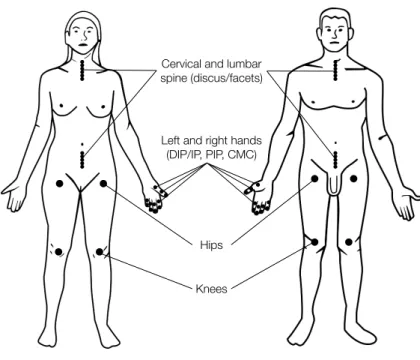
Osteoarthritis (OA) is a disabling common late onset disease of the joints char-acterized by cartilage degradation and the formation of new bone [Meu97; Riy06; Min07]. The joint damage is caused by a mixture of systemic factors that predis-pose to the disease and of local mechanical factors. Together, these factors may

dictate thedistribution and theseverity.

First, regarding thedistribution of OA, although OA can occur at any joint,

it is most commonly observed in the lumbar and cervical spine, hands, knees and

hips. Further, when a single joint is affected, OA is viewed aslocalised but when

there are multiple joints affected, it is considered to begeneralised.

Second, regarding theseverity of OA, its diagnosis can rely on radiographic

characteristics (ROA) as specified by Kellgren and Lawrence in [Kel57]: the sever-ity of the radiographic features is scored in terms of a five-points ordinal grading

Figure 1.1: Radiograph of (A) normal and (B) osteoarthritic femoral head. Radio-graphic image of osteoarthritic joints shows marginal osteophytes, change in shape of bone, subchondral bone cysts, and focal area of extensive loss of articular cartilage (with permission [Die05]).

by joint pain, tenderness, limitation of movement, friction sensation between bone and cartilage, occasional effusion, inflammation.

The incidence of ROA may result ofsystemic factors like age, gender,

genet-ics, bone density and obesity but also of local factors like joint injury, muscle

weakness, malalignment and developmental deformity. However, clinical

symp-toms and radiographic characteristics of OA often correlate poorly. In fact, the

prevalence of symptomatic OA is considerably lower than the one of ROA because of the high proportion of subjects not having joint pains.

For these reasons, OA is now regarded as a group of disctinct overlapping diseases whose particular phenotype may reflect different pathological processes.

As a result, OA is referred to as acomplex diseasesince both environmental and

genetic determinants influence its aetiology. It is likely that most individuals are affected by OA because of a combination of environmental and genetic factors.

Why subtypingOA? Our investigations may allow to study the spread of the

elucidate the clinical heterogeneity of OA and therefore enhance the identification of the disease pathways (genetics, pathophysiological mechanisms).

Patients We will consider a study called GARP which consists of Caucasian

sib-ling pairs of Dutch ancestry with predominantly symptomatic OA at multiple sites; more background on GARP and already published work can be found on-line [LUM08a]. Here we describe the study briefly.

Symptomatic OA of a joint was defined as the presence of symptoms of OA and ROA. The scoring of symptomatic OA was previously described in [Riy06]. Probands (ages 40-70 years) and their siblings had OA at multiple joint sites of the hand or in two or more of the following joint sites: hand, spine (cervical or lumbar), knee or hip. Subjects with symptomatic OA in just one site were required to have structural abnormalities in at least one other joint site, defined by the presence of ROA in any of the four joints or the presence of two or more Heberden’s nodes, Bouchard’s nodes, or squaring of at least one carpometacarpal joint on physical examination.

!"#$%&'()'*+)(,-.'#) /0%*")1+%/&,/23'&"4/5

6"34)'*+)#%784)8'*+/) 19:;2:;<);:;<)!=!5

>%0/

?*""/

Figure 1.2: The different joint locations assessed for ROA.

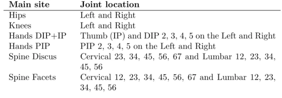
ordinal grading scheme [Kel57]. As some individuals had an incomplete ROA phenotype, they were discarded and we also decided to restrict our analysis to family sibships involving only two members (proband / sibling); we left out a total of 13 individuals. Therefore, for the analysis presented in this thesis, we

analysed the ROA profiles of 211 sibling pairs (N = 422 patients).

Table 1.1: Table describing the 45 joint locations where the individuals were measured.

Main site Joint location

Hips Left and Right

Knees Left and Right

Hands DIP+IP Thumb (IP) and DIP 2, 3, 4, 5 on the Left and Right

Hands PIP PIP 2, 3, 4, 5 on the Left and Right

Spine Discus Cervical 23, 34, 45, 56, 67 and Lumbar 12, 23, 34,

45, 56

Spine Facets Cervical 12, 23, 34, 45, 56, 67 and Lumbar 12, 23,

34, 45, 56

1.3

P

a

r

k

i

nson’s d

i

sease

Parkinson’s disease (PD) is a degenerative disorder of the central nervous system that often impairs the sufferer’s motor skills and speech, as well as other functions [Jan08]. In the following two paragraphs, we give further characteristics of PD taken from the online article of PD on the Wikipedia [Wik08]:

PD is characterized by muscle rigidity, tremor, a slowing of physi-cal movement (bradykinesia) and, in extreme cases, a loss of physiphysi-cal movement (akinesia). The primary symptoms are the results of de-creased stimulation of the motor cortex by the basal ganglia, normally

caused by the insufficient formation and action of dopamine1_{, which is}

produced in the dopaminergic neurons of the brain. Secondary symp-toms may include high level cognitive dysfunction and subtle language problems. PD is both chronic and progressive.

PD is the most common cause of chronic progressive parkinsonism, a term which refers to the syndrome of tremor, rigidity, bradykinesia and postural instability. PD is also called ”primary parkinsonism” or ”idiopathic PD” (classically meaning having no known cause although

this term is not strictly true in light of the plethora of newly discov-ered genetic mutations). While many forms of parkinsonism are ”id-iopathic”, ”secondary” cases may result from toxicity most notably of drugs, head trauma, or other medical disorders. The disease is named after the English physician James Parkinson; who made a detailed de-scription of the disease in his essay: ”An Essay on the Shaking Palsy” (1817).

Why subtypingPD? Among the PD patients, there is marked heterogeneity, both

in presence and severity of different impairments and in other variables like age at onset or family history. The progression and course of PD vary widely among individual patients and understanding more about these PD subtypes and how they relate to an individual’s disease course could improve patient treatment with existing therapies and help develop new treatments (e.g. see [MJF08] PD-subtype research program). Until now, studies on heterogeneity that are using a large cohort of patients and that are assessing the full spectrum of PD are lacking.

Data acquisition We will use data from both the PROPARK (PROfiling

PARKin-son’s disease) and the SCOPA (SCales for Outcomes in PArkinsons disease) projects. In order to evaluate the longitudinal course of PD, the PROPARK project was started in 2003 [LUM08b]. In this study, a cohort of 420 patients is screened annually on: the whole spectrum of impairments, the problems related to daily living activities and the quality of life. These instruments of measure are derived from the SCOPA project which purpose was to evaluate and / or to develop valid and reliable instruments that are specific for PD, for more details see [LUM08b; Mar03b; Mar03c; Vis04; Mar04; Vis06; Vis07].

Cohortrecruitment We first describe how the cohort was recruited. It is stemming

from patients from two university hospitals (Leiden and Rotterdam) and nine regional hospitals in the western part of the Netherlands.

As presented in [Roo08a], the diagnosis of PD was made according to the United Kingdom Brain bank criteria by a movement disorder specialist [Gib88]. The clinical diagnosis of PD was verified at each assessment. During follow-up, patients who developed symptoms and signs that pointed towards other forms of parkinsonism, were excluded from the cohort. Furthermore, participating patients had to be able to comprehend the Dutch language. Patients were not excluded from the SCOPA-PROPARK cohort based on their comorbidity and therefore the cohort provides a better reflection of the general PD population than most trial cohorts.

For the study on subtypes, patients having undergone stereotactical surgery were excluded because of potential confounding effects. At baseline, patients were

stratified based on age at onset (</ >50 years) and disease duration (</ >

and medication-induced complications [Kos91]. To avoid a bias towards recruiting the less severely affected patients and to decrease the drop-out rate, more severely affected patients were offered an assessment at home. All patients gave written informed consent to participate in the study.

Table 1.2: Measures of impairments of Parkinson’s disease in the SCOPA-PROPARK cohort.

Cognitive functioning: SCOPA-COG Sumscore

Memory Attention

Executive functioning Visuospatial functioning

Motor symptoms: SPES/SCOPA - motor Sumscore

Trembling Stiffness

Slowness of movement

Axial (including rise, postural instability, gait) Axial2 (including speech, freezing and swallowing) Motor complications:

SPES/SCOPA motor complications

Motor fluctuations Dyskinesia

Psychiatric functioning: SCOPA-PC items 1-5, Psychotic symptoms Autonomic functioning:

SCOPA-AUT Sumscore

Gastro-intestinal dysfunction (reduced to three items: full quickly, obstipation, hard strain)

Urinary dysfunction Cardiovascular dysfunction

Nighttime sleepiness: SCOPA-sleep night-time sleeping Sumscore Daytime sleepiness: SCOPA-sleep daytime sleepiness Sumscore Depression: Beck Depression Inventory Sumscore

Assessments The annual assessments encompassed self-assessed scales that

pa-tients completed at home as well as a supplementary examination consisting of researcher-administered assessment scales in the LUMC (Leiden University Med-ical Center), see Table 1.2 and [Mar03b; Mar03c; Vis04; Mar04; Vis06; Vis07] for details. In addition, socio-demographics, age at onset, disease duration, and fa-milial occurrence of PD was recorded at baseline. At each assessment, medication was recorded. Patients were optimally treated and the assessments were executed while the patients are in the so-called on state.

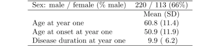
Datasetusedinthethesis The participants, have a baseline measurement and are

Table 1.3: Description of the dataset for the subtyping analysis on year one (N= 333).

Sex: male / female (% male) 220 / 113 (66%) Mean (SD)

Age at year one 60.8 (11.4)

Age at onset at year one 50.9 (11.9)

Disease duration at year one 9.9 ( 6.2)

analysis on year one were conducted on 333 patients. In Table 1.3, we describe the dataset characteristics for year one. For further details consult [Roo08a].

1.4

D

r

ug d

i

scove

r

y

A drug is a synthetic or natural substance used as, or in the preparation of, a

medication [...], for use in the diagnosis, cure, treatment, or prevention of disease

[lon84].

In this thesis, we conductedsubtyping analyses in the field of drug discovery

based on a list of banned stimulating drugs (i.e. molecules) in sports. This list is

maintained by the World Anti Doping Agency (WADA,www.wada-ama.org);

here, we use the list of 2008.

Why subtypingmoleculardatabases? Subtype discovery of chemical databases may

help to understand the relationship between bioactivity classes of molecules, thus improving our understanding of the similarity (and distance) between drug- and chemical-induced phenotypic effects.

Calculatingtheproperties ofmolecules In order to build statistical models of

mol-ecules, they first need to be described in a format understandable by computer algorithms. This step is usually referred to as the calculation of molecular ”de-scriptors”. These properties can serve as numerical descriptions (features) of molecules in other calculations like QSAR (Quantitative Structure-Activity Re-lationships), diversity analysis, combinatorial library design and in this thesis,

subtyping. In our work, we used descriptors as implemented in MOE

(Molecu-lar Operating Environment) [CCGI08]. However, there are many possible sets of features because any molecular property may be used as a molecular descriptor.

These properties are of three types. First, there are 2D descriptors which

only use the atoms and connection information of the molecule for the calcula-tion. They can be calculated from the connection table of a molecule; therefore,

they do no depend on the conformation of a molecule. Second, there areinternal

coordinates are considered invariant to rotations and translations of the

conforma-tion. Third, there are theexternal 3D descriptors (x3D) where the 3D coordinate

information is also used but this time in an absolute frame of reference. A frame of reference can be a receiving molecule to which the molecules should bind them-selves; yet, as several orientations are possible, the most likely one is determined

by adocking-method.

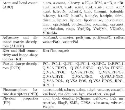
Selectedmolecularproperties In this thesis we conductsubtyping analyses on 2D

molecular properties; we do not use the 3D descriptors. In Table 1.4, we list the six classes of descriptors for which we selected a number of molecular properties; these properties are explained in Tables A.1, A.2, A.3, A.4, A.5 and A.6, which can be found in Appendix A of this thesis.

Table 1.4: 2D molecular properties that we selected to describe and characterize the databases of molecules.

Atom and bond counts

(ABC) a aro, a count, a heavy, a IC, a ICM, a nB, a nBr,a nC, a nCl, a nF, a nH, a nI, a nN, a nO, a nP,

a nS, b 1rotN, b 1rotR, b ar, b count, b double, b heavy, b rotN, b rotR, b single, b triple, chiral, chiral u, lip acc, lip don, lip druglike, lip violation, nmol, opr brigid, opr leadlike, opr nring, opr nrot, opr violation, rings, VAdjEq, VAdjMa, VDistEq, VDistMa

Adjacency and dis-tance matrix descrip-tors (ADDM)

balabanJ, diameter, petitjean, petitjeanSC, radius, weinerPath, weinerPol

Kier and Hall connec-tivity and kappa shape indices (KH)

KierFlex, zagreb

Partial charge

descrip-tors (PCD) PC., PC..1, Q PC., Q PC..1, Q RPC., Q RPC..1,Q VSA FHYD, Q VSA FNEG, Q VSA FPNEG,

Q VSA FPOL, Q VSA FPOS, Q VSA FPPOS,

Q VSA HYD, Q VSA NEG, Q VSA PNEG,

Q VSA POL, Q VSA POS, Q VSA PPOS, RPC., RPC..1

Pharmacophore

fea-ture descriptors (PFD) a acc, a acid, a base, a don, a hyd, vsa acc, vsa acid,vsa base, vsa don, vsa hyd, vsa other, vsa pol

Physical properties

(PP) apol, bpol, density, FCharge, logP.o.w., logS, mr,reactive, SlogP, SMR, TPSA, vdw area, vdw vol,

Datasetusedinthethesis The dataset is composed of substances taken from the 2008 WADA Prohibited List together with molecules having similar biological activity and chemical structure from the MDL Drug Data Report database; it was generated by Edward O. Cannon. In previous work [Can06a; Can06b; Can08], the purpose was to partition the space of chemical substances into subgroups of bioactivity classes using classification algorithms; the dataset used was the

wada2005dataset which is based on the 2005 prohibited list. In this work, we

use clustering algorithms to identify the subgroups.

The molecules may belong to one of the ten activity classes: theβ blockers,

anabolic agents, hormones and related substances,β-2 agonists, hormone

antag-onists and modulators, diuretics and other masking agents, stimulants, narcotics, cannabinoids and glucocorticosteroids. Then, the molecules were imported into MOE from which all 184 two dimensional descriptors were calculated. We embed

thewada2008dataset within ourR SubtypeDiscoverypackage.

1.5

C

onc

l

ud

i

ng

r

e

m

a

r

ks

We presented three domains where subtyping can be used to enhance the under-standing of the problem.

In OA, the aim of subtyping is to study the spread of the disease across different joint sites and to show whether it is stochastic or follows a particular pattern (subtype).

In PD, as the spread and the course of PD vary widely among individual patients, understanding more about these PD subtypes could improve patient treatment with existing therapies and help develop new treatments.

In drug discovery, subtyping chemical databases may help to understand the relationship between bioactivity classes of molecules, thus improving our under-standing of the similarity (and distance) between drug- and chemical-induced phenotypic effects.

Chapter

2

A

S

ce

n

a

r

i

o

f

o

r

Sub

t

yp

e

D

i

s

c

ov

e

r

y

by

C

l

us

t

e

r

An

a

l

ys

i

s

In this chapter, we present oursubtyping scenario. First, we discuss data

process-ing issues when preparprocess-ing the data before analysis. Next, we motivate our choice for a particular clustering method. Then, to select for a number of subtypes or a model, we describe a computational approach that repeats data modeling. Fi-nally, we report on methods to characterize, compare and evaluate the most likely subtypes.

2.1

I

n

t

r

oduc

ti

on

To identify homogeneous subtypes of complex diseases like Osteoarthritis (OA) and Parkinson’s disease (PD) and to subtype chemical databases, we developed a scenario mimicking a cluster analysis process: from data preparation to clus-ter evaluation, see Figure 2.1 for an illustration of our scenario. It implements various data preparation techniques to facilitate the analysis given different data processing. It also features a computational approach that repeats data modeling in order to select for a number of subtypes or a type of model. Additionally, it defines a selection of methods to characterize, compare and evaluate the top ranking models.

!"#"$%&'%"&"#()*

!"#$%&"'()*+#%&,# !"-.#/',+01/% !",1/%'2$-'#$1, !"!2#&/$,3

+,-.#'&$"*",/.(.

!"%1(&2"4'+&("52*+#&/$,3

0)!',$.','+#()*

!"/&6&'#&("52*+#&/"%1(&2$,3 !"789"+51/&"','2:+$+

.-1#/%'$+2"&"+#'&(3"#()*$ "*!$+)0%"&(.)*

!"3/'6;$5"5;'/'5#&/$-'#$1, !"+#'#$+#$5'2"5;'/'5#&/$-'#$1, !"+#'#$+#$5'2"51%6'/$+1, !"+*4#:6&"/&6/1(*5$4$2$#:

.-1#/%'$.#"#(.#(+",$ '4",-"#()*

!"<=>?"2'%4('"+$4+ !"<=>?"311(,&++"10"!#"#&+# !"<(/*3"($+51@&/:?"9;$A"%'/3$,'2+

Figure 2.1: Workflow of a subtype discovery analysis.

2.2

Da

t

a

p

r

epa

r

a

ti

on

and

c

l

us

t

e

r

i

ng

We aim to identify homogeneous and reliable subtypes. Hence, cluster results

should be reproducible and the clusters should characterize true underlying

pat-terns, not the incidental ones. We discuss in this section the removal of thetime

dimension in the OA and PD datasets, thereliabilityandvalidityof cluster results

and give a brief overview of model based clustering.

2

.

2

.

1

D

a

t

a

p

r

e

p

a

r

a

t

i

on

As data preparation can influence largely the result of data analysis, our scenario implements various methods to transform and process data, e.g. computing the z-scores of variables to obtain scale-invariant quantities, normalizing according

to the Euclidean norm (L2), the Manhattan distance (L1), the maximum and

centering with respect to the empirical mean, the median or the minimum. As in the overal severity of OA and PD, respectively age or disease duration

(thereafter, thetime) are known to play a major role, we may want to remove their

!" #$% & '()*+ '()%* '(),% '()-, '()&-'()"& .()%* .(),% .()-, .()&-.()"& '()*+ '()%* '(),% '()-, '()&-'()"&

# " &

-!"#$%&'(')"*$+,%&-+ !.#$/'0-$"123+/-1$+,%&-+ (/01234562734567893:;<=>3:?@?>*=36ABC729392CBA7 .()%* .(),% .()-, .()&-.()"& *3:&D= ,3:-E= %3:--= &3:DD= "3:%"= -3:"D-= *3:"+= %3:*,= ,3:D%= -3:+-= &3:,#= "3:",-=

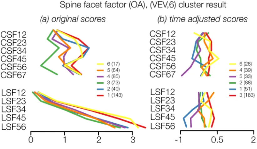
Figure 2.2: For OA, we show results of two cluster analyses on the spine facets factor with a VEV model having six mixtures (the VEV model will be explained in section 2.2.3). In (a), the modeling is on the original ROA scores, i.e. between[0,4]and in (b), on the time adjusted scores, i.e. z-scores. This illustrates how the time influences the cluster results. The arrangement of the variables mimicks the disposition of the cervical and lumbar vertebrae, from top to bottom.

by them. In Figure 2.2, we report a visualization of two cluster analyses on OA data: we conducted the clustering on the original scores and on the time adjusted scores; it shows how much the time influences the modeling. So, to remove the

time dimension for the data, we first perform regression on the time for each

variable and next, we conduct cluster analyses on the residual variance.

If we denote by α and β the estimated intercept and coefficient vectors of

the regression, by the matrix X the data where xij refers to measurement j of

observationi, then the regression is given by

xij(ti) =αj+βjg(ti) +εij, (2.1)

εij =xij(ti)−αj−βjg(ti). (2.2)

The εij refer to the residual variation and g(t) ∈ !log(t),

√

t, t, t2_{, exp(t)}" _(the

time effect is not necessarily linear). Additionally, residualsεij should distribute

normally around zero for each variablej, as illustrated in Figure 2.3.

2

.

2

.

2

T

h

e

r

e

li

a

b

ili

t

y

a

nd v

a

li

d

i

t

y o

f

a c

l

us

t

e

r r

e

su

l

t

In our data mining scenario for subtype discovery by cluster analysis,

hierar-chical clustering [Sne73] or k-means [Has01] did not match our expectations in

!"#$%&$'(&")*+,-%

! " #

! $!! "!!

%!! !+,++-./,/0-.10+.23453675.8(9:*4!"#$%&'()*

! $!! "!! %!!

! "&'

("&'

!"#$%&'%()'#*+,-.&

! "! #!

! '! $!! $'!

!!"#$%&'%()'#*+,-.&

! " #

! "! #! )!

!"#$%&'()*$+",-"./0$!12#3$ 4,-5-6"/$784,07

!.#$%&'()*$+",-"./0$!12#3$ 9-:0$";<=790;$784,07

!8#$%2>1?@A*$+",-"./0$!BC#3$ 4,-5-6"/$784,07

!;#$%2>1?@A*$+",-"./0$!BC#3$ 9-:0$";<=790;$784,07

Figure 2.3: These four figures illustrate the original and the time-adjusted data distri-butions of variables DIP5 L and beck, which respectively pertain to OA and PD analyses. Such histograms are obtained when plotting a dataset class (cdata) of the R Subtype-Discovery package. To be valid, the residualsεij of the regression on the time should

distribute normally around zero for each variablej.

based clustering that relies on the EM-algorithm (Expectation Maximization) for parameter estimation [Fra99; Fra02b; Fra03; Fra06]. In the following two

para-graphs, we discuss thereliabilityandvalidity of thek-means, the hierarchical and

the model based clustering.

k-meansand hierarchicalclustering First, in terms ofreliability, the cluster results should be consistent when we repeat the analysis. For example, when we repeat

thek-means, solutions may differ because of the different starting values. Second,

both the hierarchical clustering and the k-means clustering depend on distance

measures which do not necessarily mimic the data distribution of the clusters;

however, to bevalid, the clusters should be understandable which is not evident

Figure 2.4: On the left, we show a simple modeling with three mixtures in two dimen-sions which are defined by their centerµk and their geometryΣk withk = 1,2,3. On

the right, we illustrate two mixtures on a single dimension. Membership of the gray is most likely. Membership of the black is less likely.

In fact, the clusters should also be distinguishable, which becomes an issue as the modeling takes place in higher dimensions because the distance-based algo-rithms are sensitive to the curse of dimensionality [Bey99]. And finally, another aspect that hampers especially the hierarchical clustering, concerns the numerous parameters that can only be set subjectively. The book [Sne73] gives a detailed description of all the possible parameters.

Modelbased clustering To be fair, reliability issues also exist for clustering by

mixture of Gaussians because it relies on the EM-algorithm. To estimate model parameters, EM optimizes iteratively the model likelihood and as a matter of fact, different starting values for EM may lead to different cluster results. Therefore, an important issue concerns the sensibility to different starting values of the mixture modeling. In this regard, Fraley and Raftery decided to initiate systematically their EM-algorithm by a model based hierarchical clustering [Fra99]. This choice ensures the reproducibility of the cluster results because two repeats of the mixture modeling will initiate EM equally.

Concerning thevalidityissue, mixture modeling not only reports the estimated

2

.

2

.

3

Cl

us

t

e

r

i

ng by

a

m

i

x

t

u

r

e

o

f

G

a

uss

i

a

ns

In this subsection, as in [Fra99; Fra02b; Fra03; Fra06], we describe clustering by mixture modeling.

First, the likelihood function of a mixture of Gaussians is defined by

LMIX(θ,τ|x) =

N

#

i=1

G

$

k=1

τkφk(xi|µk,Σk), (2.3)

where xi is the ith of N observations, G is the number of components and τk

the probability that an observation belongs to thekth _{component (henceτ}

k ≥0

and ΣG

k=1τk = 1). Then, the likelihood of an observationxi to belong to thekth

component is given by

φk(xi|µk,Σk) =

exp_{−1

2(xi−µk)

T_Σ−1

k (xi−µk)}

%

det(2πΣk)

. (2.4)

The reparameterization proceeds by eigenvalue decomposition of the covariance

matrix Σk

Σk=DkΛkDTk. (2.5)

This decomposition depends on the diagonal matrix Λk of the eigenvalues and

on the eigenvector matrix Dk which determines the orientation of the principal

components. The matrix Λk can be decomposed further into

Λk =λkAk (2.6)

withAk the geometrical shape andλk the largest eigenvalue.

In their framework, Fraley and Raftery control the structure of Σk using

con-straints on the three parametersλk, AkandDk. The constraints are expressed in

letters_{I, E, V}which stand for identical, equal and variable respectively.

λk refers to the relative size or thescaleof thekthmixture which may be

equal for all mixtures (E) or vary (V).

Ak specifies thegeometrical shapewhich may limit the mixtures to

spher-ical shapes (I), to equally elongated shapes for all mixtures (E), or to varying ones (V).

Dk characterizes the principal orientations of the covariance which may

simply coordinate along the axes (I) and therefore neglect estimation of the covariates; but when considering covariates, we may select an equal orientation for all mixtures (E) or a different one (V).

EM-algorithm For a given number of mixtures and a covariance model, the EM-algorithm is used to estimate the model parameters [Dem77]. It alternates

iter-atively between a step ofExpectation to estimate for each observation its cluster

membership likelihood, and a step of Maximization to identify the parameters

that maximize the model likelihood. The iterative process stops as likelihood improvements become small.

An important concern for the EM algorithm is the dependency on the starting point. As mentioned before, Fraley and Raftery propose to systematically initial-ize EM with a model based hierarchical clustering. Though, a common strategy is to start EM from several random points and then to study the sensibility of the cluster results to these changes. We selected this second strategy for our data mining scenario.

2.3 M

ode

l

se

l

ec

ti

on

The larger the number of parameters, the more likely it is that our model may overfit the data which restricts its generality and comprehensiveness. In this section, we discuss a score that we use as a guidance to compare models

involv-ing different numbers of parameters and an approach to conduct avalid model

selection.

2

.

3

.

1

A

s

c

o

r

e

t

o

c

o

m

p

a

r

e

m

od

e

l

s

For model selection, Kass and Raftery [Kas95] prefer the Bayesian Information Criterion (BIC) to the Akaike Information Criterion (AIC) because it approxi-mates the Bayes Factor. Therefore, our analyses also rely on the guidance pro-vided by the BIC. It is defined by

BIC=−2 logLMIX+ log (N×#params), (2.7)

with_LMIXthe Gaussian-mixture model likelihood,Nthe number of observations

and #paramsthe number of parameters of the model.

2

.

3

.

2

Va

li

d

m

od

e

l

s

e

l

ec

t

i

on

In our data mining scenario, we found it inappropriate to conduct model selection on the basis of a single BIC value because it left several questions unanswered. We give some of them:

1. What is the statistical significance of BIC scores differences that are less than 5%?

3. Did the EM-algorithm end in a local or a global likelihood maximum?

For this reason, we decided to further validate our choice for a particular model by repeating the data modeling process for different starting values; our approach proceeds as follows:

1. Set an integer that fixes the starting point of the random number generator.

2. Draw from a uniform distribution a matrix of cluster membership probabil-ities.

3. Proceed to amaximization step (M-step) to identify the parameters of the

most likely model.

4. Start EM-algorithm from itsexpectation step (E-step).

This way, by repeating EM initialization from many different starting points, we

can select the most likely model and consider it as theoptimal one.

Then, to conduct a valid model selection, we aggregate the BIC scores in a number of ways. In first place, we report the average rank of the model (re-spectively the average rank of the number of clusters) when a particular number of clusters (resp. a model-type) is chosen. These rankings may enable to select for a particular type of model and a number of clusters. We also report tables

that characterize statistically the BIC scores in terms of the empirical mean,

the standard deviation and different quantile statistics. Finally, two more tables present the starting values and the BIC scores of the most likely models for each combination.

2.4

C

ha

r

ac

t

e

r

i

z

i

ng

,

co

m

pa

r

i

ng

and

eva

l

ua

ti

ng

c

l

us

t

e

r r

esu

lt

s

Because cluster models may take different spatial-shapes, we need methods to report their characteristics and to compare them. Further, when analysing data from the medical domain, we consider as important to evaluate the clinical rel-evance of the subtypes by some additional characteristics. Therefore, in this section, we present our techniques to address these different aspects.

2

.

4

.

1

V

i

su

a

li

z

i

ng sub

t

yp

e

s

To check the effect of changing the settings (the type of cluster model and the number of clusters), we need visualization tools to see the characteristics of the cluster results. Being influenced by Tukey [Tuk77] and Tufte [Tuf83; Tuf90] for scientific data visualization and by Brewer’s suggestions for color selection in

geography [Bre94], we selected three visual-aids to address this issue: heatmaps

Heatmaps In the analysis of micro array data, heatmaps are often used to display and cluster data. However, as heatmaps depend on hierarchical clustering, there are many parameters that need to be set rather subjectively. Besides, as we do calculations with distance measures, the variables should be scale-free and comparable; this may be awkward when variables are not scale-homogeneous. On top of that, as variables are correlated, the distances will mostly reveal patterns in the principal component dimensions of the data.

For the OA data, we can illustrate this by considering a large joint factor that consists of hips and knees and another one that consists of the spine joints. Simply because there are only four variables in the first factor and about 20 in the second, the spine has a larger ”contribution” than the large joints in the distance. So, simple distances lack sensitivity to manifest changes in the small principal component dimensions. We limit the use of heatmaps to report statistical patterns of the clusters, e.g. the mean, the median or quantiles.

Next, as hip left and right pertain to the hips in OA or as both urinary and cardiovascular problems reflect autonomic symptoms in PD, we can often group variables into main factors. Indeed, we may expect the variables to correlate in each factor; yet, standard heatmaps do not exploit the grouping of the variables, this makes the comprehesion of the cluster results more difficult.

Parallel coordinateplots In parallel coordinates plots, we can make use of this

grouping information in factors to order the variables appropriately. For each cluster, we use a different color and, as Figure 2.2 illustrates OA data, we

char-acterize each center (µk) by lines connecting the different variables (the parallel

axis). In this Figure, we notice the particular ordering for the cervical and the lumbar spinal joints that reflects the natural ordering of these joints from top to bottom. An interesting additional property of this type of plots is that besides each cluster center (the mean pattern), we can also report quantile-statistics us-ing connected lines of a different shape (e.g. the 2.5% and 97.5% patterns of a cluster).

Dendrograms Finally, in spite of the many disadvantages of hierarchical

cluster-ing, we find it a useful addition to the heatmaps and parallel coordinates because dendrograms can illustrate the similarity between the center patterns or between the variables. In fact, a dendrogram on the cluster centers can help to order the clusters by similarity, whereas a dendrogram on the variables can provide a rudi-mentary factor analysis. Therefore, both kinds of dendrograms are included and provide additional understanding.

2

.

4

.

2

S

t

a

t

i

s

t

i

ca

l

c

h

a

r

ac

t

e

r

i

z

a

t

i

on

a

nd

c

o

m

p

a

r

i

son o

f

sub

t

yp

e

s

First, using the log of the odds, we report the main statistical characteristics of

association tables from which we estimate the usualχ2 _{statistics. Next, we use}

further theχ2 _{statistics to calculate a single measure in terms of theCramer’s V}

coefficient of nominal association. Finally, as a way to assess the reproducibility

of cluster results, we estimate the generalization of the cluster result by training common machine learning algorithms on the clustered data.

Statisticalcharacterization For each application domain, we group variables by

main factor such as the main joint sites in OA (the spine facets, the spine lum-bars, the hips, the knees, the distal and the proximal interphalengeal joints), the impairment domain in PD (the cognitive, the motricity and the autonomic disorders) and the class of molecular descriptors in drug discovery. Then, to

char-acterize statistically the cluster results, we compute the odd of the cluster data

distribution as compared to the one of the dataset; the data distribution is the sum of the scores in each group of variables (the factors).

In practice, one might refer to thelog of the odds as the cross-product because

we calculate it from tables similar to Table 2.1. We express the log of the odds

of a clusterkon a factorl as

logoddskl = logA×D

B_×C. (2.8)

Table 2.1: For each sum score l, we consider a middle value δl such as the dataset

meanormedian. For cells A and B, we use it to count how many observationsiin the clusterSk have a sum score above and below its value. For cells C and D, we proceed to

a similar count but on the rest of the observationsi_∈{S₋Sk}.

xi<δl xi≥δl

i∈Sk A B

i∈{S−Sk} C D

Statisticalcomparison ofcluster results In order to compare cluster results, we re-port association tables that describe the joint distribution between the two cluster affectations of the observations (nominal variables). If the table has many empty cells, then the two cluster results are highly related. However, if the joint distribu-tion over all cells is even, then the two cluster results are unrelated (independent). Further, to summarize the association tables, we calculate the Cramer’s V.

Similarly to Pearson’s correlation coefficient, the Cramer’s V takes values in [0,1];

one stands for completely correlated variables and zero for stochastically

nominal association. Therefore, the more unequal the marginals, the more V will be less than one. Alternatively, the measure can be regarded as a percentage of the maximum possible variation between two variables. It is defined by

V =

&

χ2

n_×m, (2.9)

where nis the sample size and m=min(rows, columns)−1.

In our table-charts, we will embed in the top left the joint distribution and in

the lowest row theCramer’s V coefficient.

Estimatingthe cluster resultreproducibility When performing unsupervised cluster

analysis, it is important to know whether the cluster result generalizes, for instance to the total patient population in the case of medical research. Therefore, we chose

to assess the cluster result learnability by training machine learning algorithms

like the naive Bayes, the linear Support Vector Machines or, as a baseline, the one nearest neighbor classifier.

To evaluate these algorithms, we use the average classifier accuracy estimated by training ten times the classifiers on datasets splitted randomly into training (70%) and test set (30%). To split the data, we chose to preserve in every training and test set the cluster proportions from the original sample.

Stratifying the samples enables to reduce the variability of the accuracy esti-mates which is coherent with the practice in machine learning because we primar-ily aim to compare algorithms. However, in medical research, we might prefer to include the variability inherent to the cluster proportions in the estimation of the accuracy.

2

.

4

.

3

S

t

a

t

i

s

t

i

ca

l

e

v

a

l

u

a

t

i

on o

f

sub

t

yp

e

s

When conducting a subtype discovery analysis, a key concern is the evaluation of the clusters. For that purpose, we implemented a simple mechanism to add study-specific evaluation procedures of the clusters.

In OA for instance, as the study involves sibling pairs, we defined two sta-tistical tests that assess the level of familial aggregation in each subtype and its

significance. Our first test relies on a risk ratio which we refer to as the λsibs,

whereas the second test makes use of aχ2_{-test of goodness of fit.}

In drug discovery,χ2 _{cell-statistics between the human-defined classification}

and the one identified by the subtyping are reported; we search forχ2_{cell-statistics}

showing a large marginal.

TheλsibsriskratioinOAresearch First of all, we characterize each individual as

proband or sibling depending on whether this individual was the first sibling

Then, this test quantifies the risk increases of the second sibling given the

characteristics of the proband. For instance, aλsibs= 1 means that the risk does

not increase and that the cluster membership of the proband does not influence

the one of his sibling. On the other hand, ifλsibs = 2, then the risk increase is

two-fold. Finally, aλsibsis significant when the lower bound of the 95% confidence

interval is above 1. In the following, we describe formally theλsibsand we derive

its confidence interval analytically by the delta method.

Take two siblings s1 and s2 with s1 being the proband. A proband is the

first affected family member who calls for medical attention. We consider the

probability of a sibling to belong to a groupSk asP(si∈Sk) withi∈{1,2}, or

for shortP(si). Then, the conditional probability that the second sibling is inSk

given that the first sibling is also inSk is referred to asP(s2|s1). Therefore, the

λsibs is expressed by

λsibs(Sk) =

P(s2|s1)

P(s2)

= P(s1, s2)

P(s1)P(s2)

=P(s1, s2)

P(s)2 . (2.10)

where P(s1) =P(s2) =P(s) if the population is considered to be infinite. Next,

we derive a confidence interval by the delta method using

λsibs=

ˆ α ˆ

β (2.11)

where ˆα= P(s1, s2), ˆβ = P(s) (the hat denotes quantities estimated from the

data). Then, the variances and covariance of ˆα,βˆhave the form

σ2α=

ˆ

α(1−α)ˆ

ni

, (2.12)

σ2

β =

ˆ

β(1₋β)ˆ

N , (2.13)

cov(ˆα,βˆ) =α(1ˆ −β)ˆ

N , (2.14)

withnithe sibship size andN the number of observations. The first order Taylor

approximation off(α,β) in (ˆα,β) is expressed byˆ

f(α,β) =f(ˆα,βˆ) + $

δ=α,β

(δ₋ˆδ)∂f(ˆα,β)ˆ

∂δ +R1. (2.15)

If we move the zeroth derivative to the left and we raise everything to the square, then we obtain

'

f(α,β)₋f(ˆα,β)ˆ (2=

)

(α₋α)ˆ ∂f(ˆα,β)ˆ

∂α + (β−βˆ)

∂f(ˆα,β)ˆ

∂β

*2

. (2.16)

Provided that∂f(ˆα,β)/∂αˆ = 1/βˆ2 _{and∂f(ˆα,β}ˆ_)/β=