BAYESIAN MAXIMUM ENTROPY INTEGRATION OF OZONE OBSERVATIONS AND AIR QUALITY MODEL PREDICTIONS FOR IMPROVED EXPOSURE ESTIMATES
Yadong Xu
A dissertation submitted to the faculty at the University of North Carolina at Chapel Hill in partial fulfillment of the requirements for the degree of Doctor of Philosophy in the Department of Environmental Sciences and Engineering in the Gillings School of Global Public Health.
Chapel Hill 2016
Approved by:
William Vizuete
Marc Serre
Sarav Arunachalam
Jason West
ii © 2016 Yadong Xu
iii ABSTRACT
Yadong Xu. Bayesian Maximum Entropy Integration of Ozone Observations and Air Quality Model Predictions for Improved Exposure Estimates
(Under the direction of William Vizuete and Marc Serre)
To support the Women’s Health Initiative (WHI) Memory Study (WHIMS), a nationwide cohort
study, accurate ozone exposure estimates for ambient concentrations needed to be generated at a national
scale for years 1993-2010. For this large spatial and temporal coverage we investigated different
geo-statistical approaches to generate estimates that integrate routine monitoring from surface ozone
observations and episodic chemical transport model (CTM) outputs. The goal is to take advantage of the
accuracy of the observational data and the continuous spatial/temporal coverage of CTM model outputs.
In this work, we demonstrate a Bayesian Maximum Entropy (BME) data integration geo-statistical
approach for making national scale ozone estimates that models the non-linear and non-homoscedastic
relation between air pollution observations and CTM predictions. This is the first application of BME that
fully accounts for variability in CTM model performance through our novel Regionalized Air Quality
Model Performance (RAMP) approach. A validation analysis was completed using only non-collocated
data outside of a validation radius 𝑟𝑣 and the error statistics between observations and re-estimated values
were obtained. We show that by accounting for the spatial and temporal variability in model performance
there is 3-12 fold increase in R2 (the squared Pearson correlation coefficient) percentage change for the
daily ozone concentrations compared to estimates that assume model performance does not change across
space and time.
Our second project is to investigate the differences of the predictive capacity for two upscaling
methods: USM1 (data aggregation from hourly to daily followed by BME approach estimation) and USM2
iv
computationally intensive method USM1 outperforms the method USM2. This highlights the capability
of the RAMP approach that was able to capture the spatial temporal variability in CTM model performance
at time scale of interest. Thus, we recommend to use upscaling method USM1 to integrate CTM model
predictions through RAMP approach because USM1 can achieve higher estimation accuracy and also
v
vi
ACKNOWLEDGEMENTS
I would like to thank my advisors, Dr. William Vizuete and Dr. Marc Serre for their guidance and
mentorship. I greatly appreciate their trust of giving me the opportunity to work on the research project for
the Women’s Health Initiative (WHI) memory study. Their knowledge and expertise facilitated successful
model development and analysis. Without their help, we could not have finished the WHIMS project
successfully. I also would like to thank my committee member, Dr. Sarav Arunachalam, Dr. Jason West
and Dr. Karin Yeatts for their feedback and helpful suggestions.
I would like to express my deepest gratitude and appreciations to my husband Morris and my son
Haoran for their continuous support and encouragement during this long journey. Thank them for believing
in me and providing a quiet and pleasant environment at home during long hours of model development
and manuscript writing. I am also deeply grateful to my extended family and friends for their support and
care.
I am thankful for the support I received from my department’s administrative staff, particularly
Jack Whaley, who always answered my questions promptly and provided great help in my class registration
and academic development.
I am also thankful to my research classmates/colleagues in the CHAQ/MAQ/BME labs for the great
learning environment we shared. I am especially grateful to Pradeepa Vennam and Matt Woody for their
help in regards to CMAQ/CAMx post analysis tools. I am thankful to Dr. Yasuyuki Akita and Jeanette
Reyes from BMElab for sharing their expertise in BMElib, geo-statistics and also MATLAB programming.
I would like to acknowledge the National Institute on Aging (NIA) of the National Institutes of
vii
Sciences (NIEHS) training program (grant number T32ES007018) of NIH for providing me with financial
viii
TABLE OF CONTENTS
LIST OF TABLES ... xii
LIST OF FIGURES ...xiii
LIST OF ABBREVIATIONS AND SYMBOLS ... xx
CHAPTER 1 – INTRODUCTION ... 1
1.1Ozone estimates for epidemiologic studies ... 2
1.2Environmental sources of ozone data ... 4
1.3Geo-statistical approaches for integration of environmental data from multiple sources ... 6
1.4Thesis Hypothesis and approach ... 8
CHAPTER 2 – BAYESIAN MAXIMUM ENTROPY INTEGRATION OF OZONE OBSERVATIONS AND MODEL PREDICTIONS: A NATIONAL APPLICATION ... 10
2.1 Introduction ... 10
2.2 Data ... 12
2.2.1 Ozone Monitoring Data ... 12
2.2.2 Air Quality Model Predictions ... 13
2.3 Methods ... 13
2.3.1 BME Estimation Methodology ... 13
2.3.2 Variability of CTM Model Performance Evaluation across the Continental US ... 16
2.3.3 The Proposed Regionalized Air Quality Model Performance (RAMP) Evaluation Framework ... 17
2.3.4 Offset analysis ... 19
2.3.5 Space-time Covariance Model ... 19
ix
2.4 Results ... 22
2.4.1 BME Ozone estimates ... 22
2.4.2 Soft data construction using the RAMP approach ... 24
2.4.3 Validation results ... 26
2.5 Discussion... 28
2.6 Acknowledgments ... 30
CHAPTER 3 – BME INTEGRATION OF OZONE OBSERVATIONS AND CTM PREDICTIONS AT MULTIPLE TIME SCALES ... 31
3.1 Introduction ... 31
3.2 Data Sources ... 33
3.3 Methods ... 34
3.3.1 BME Estimation Methodology ... 34
3.3.2 Variability of CTM Model Performance Evaluation across the Continental US ... 35
3.3.3 Regionalized Air Quality Model Performance (RAMP) Analysis for Hourly Ozone ... 36
3.3.4 Offset analysis ... 38
3.3.5 Space-time Covariance Model ... 38
3.3.6 Validation analysis ... 39
3.4 Results ... 41
3.4.1 BME Ozone estimates ... 41
3.4.2 Validation results ... 43
3.5 Discussion... 47
CHAPTER 4 – CONCLUSIONS ... 50
4.1 Scientific findings ... 53
4.2 Methodological aspects and study limitations ... 54
x
APPENDIX A – SUPPORTING INFORMATION FOR BAYESIAN MAXIMUM ENTROPY INTEGRATION OF OZONE OBSERVATIONS AND MODEL
PREDICTIONS:A NATIONAL APPLICATION ... 57
A.1 Ozone CTM model performance evaluation for daily metrics DM8A and D24A ... 57
A.1.1 CTM model performance evaluation for the DM8A ozone concentrations ... 59
A.1.2 CTM model performance evaluation for the D24A ozone concentrations ... 64
A.2 Parameter selection for the offset analysis and covariance model ... 68
A.2.1 Maps and figures of the offset analysis for the DM8A ozone concentrations ... 70
A.2.2 Maps and figures of the offset analysis for the D24A ozone concentrations ... 73
A.2.3 Covariance model ... 77
A.3 Additional results of BME O3 estimates ... 80
A.3.1 Additional maps showing the soft data for the DM8A O3 ... 80
A.3.2 Additional maps of BME O3 estimates for D24A O3 ... 81
A.4 Testing the statistical significance of the increase in R2 for the cross-validation analysis ... 85
A.5 Additional results for the cross-validation analysis ... 86
A.6 The cokriging approach with a parametric relationship between the observations and the CTM model predictions ... 88
A.7 A discussion about the limitation of using the daily averages of the hourly ozone observations as hard data ... 96
APPENDIX B – SUPPORTING INFORMATION FOR BME INTEGRATION OF OZONE OBSERVATIONS AND CTM PREDICTIONS AT MULTIPLE TIME SCALES ... 98
B.1 Hourly Ozone CTM model performance evaluation ... 98
B.2 Parameter selection for the offset analysis and covariance model ... 104
B.2.1 Offset analysis ... 104
B.2.2 Covariance model ... 109
xi
B.4 The additional results for the validation analysis... 112
B.4.1 The additional error statistics for the validation analysis... 112
B.4.2 The additional validation analyses show the influence of the grid cell resolution on the accuracy of the BME estimates……….112
APPENDIX C-WHIMS PROJECT REPORT-CODE DOCUMENTATION AND QUALITY ASSURANCE FOR THE ESTIMATION OF DAILY O3 FROM 1993 TO 2010 USING OBSERVATIONS AND CTM ... 115
C.1 Introduction ... 115
C.2 Materials ... 116
C.3 Location of the study participants ... 117
C.4 Methods ... 118
C.5 Numerical implementation... 120
C.6 Results ... 123
C.7 QA/QC ... 123
C.8 Date and version number ... 125
xii
LIST OF TABLES
Table 2. 1: Validation statistics for BME data integration scenarios OBS, CAMP, and RAMP* ... 27
Table 3. 1: The list of BME data integration simulations used in the validation analysis ... 40
Table 3. 2: Validation statistics hourly O3 for BME data integration scenarios OBS and RAMP # ... 44
Table 3. 3: Compare validation statistics for DM8A and D24A O3 between the upscaling methods USM1 and USM2 ## ... 45
Table 3. 4: Validation statistics for BME data integration scenarios OBS and RAMP using different soft data (for 888 sites only) for upscaling method USM1 ... 47
Table A. 1s: Spatial and temporal offset parameters and their label ... 69
Table A. 2s: Parameter values of the 3-structured covariance model for each offset range for DM8A O3 ... 77
Table A. 3s: Parameter values of the 3-structured covariance model for each offset range for D24A O3 ... 77
Table A. 4s: Validation statistics of MNB and MNGE for BME data integration scenarios OBS, CAMP, and RAMP ... 87
Table A. 5s: Validation statistics for BME data integration scenarios OBS, CAMP, and RAMP ... 88
Table A. 6s: Error statistics of validation analysis to compare BME with RAMP and Co-kriging with a parametric approach. ... 96
Table B. 1s: Summary of error statistics for CTM model performance at ozone monitoring sites ... 104
Table B. 2s. Spatial and temporal offset parameters and their label ... 105
Table B. 3s: Parameter values of the 3-structured covariance model for each set of offset ranges ... 109
Table B. 4s. Computational costs for generating BME ozone maps USM1 vs USM2# ... 112
xiii
LIST OF FIGURES
Figure 2. 1: RAMP analysis conducted specifically at time t=11-Jul-2005 and for sites ID 060372005(left) and 120713002(right). The empty circles show the pairs of observed-modeled values (zj, zj) that are within 120 days of t. The vertical lines show the stratification of these pairs in 10 bins. The interpolation lines connecting the filled circles and triangles show how the mean of the observed value in each bin, λ1(zb, sn, t) (filled circles), and the corresponding standard deviation, λ2(zb, sn, t) (filled triangles) change as a function of the average modeled
value zb in that bin. ... 18
Figure 2. 2. Maps of BME mean estimates (Top) and corresponding standard deviations of BME estimates (Bottom) of the DM8A ozone concentrations (ppb) on day Jul-11-2005 obtained with scenario OBS (Left), CAMP (middle panels) and RAMP (Right). Circles in the maps represent locations of monitoring sites
and color match legend for observed concentrations. ... 23
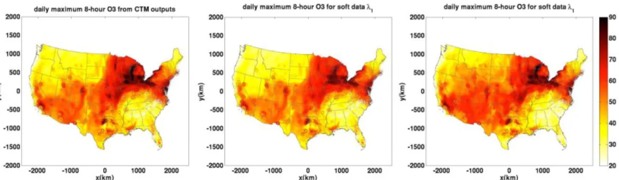
Figure 2. 3: The DM8A ozone concentrations in the United States on 11-July-2005 using (Left) the raw CTM Model predictions, (Middle) the bias-corrected expected values λ1(zi, pi) for the estimation scenario CAMP, and (Right) the bias-corrected
expected values λ1(zi, pi) for the estimation scenario RAMP. ... 25
Figure 3. 1: RAMP analysis conducted specifically at time t=11-Jul-2005 and for sites ID 060372005(left) and 120713002(right). The empty circles show the pairs of hourly observed-modeled values (zj, zj) that are within 120 days of t. The vertical lines show the stratification of these pairs in 10 percentile bins. The interpolation lines connecting the filled circles and triangles show how the mean of the observed value in each bin, λ1(zb, sn, t) (filled circles), and the corresponding standard deviation, λ2(zb, sn, t) (filled triangles) change as a function of the average modeled
value zb in that bin. ... 37
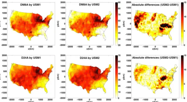
Figure 3. 2. Maps of Jul-11-2005 ozone BME estimates in ppb of the DM8A (Top) and the D24A (Bottom) obtained from upscaling method USM1 (Left) and USM2 (Middle). Also shown are the absolute differences (USM2-USM1) between these
two methods (Right). ... 42
Figure A. 1s: The ozone monitoring sites (circles), CAMx modeling domain with 36x36km2 grid cell resolution (dash-dotted line rectangle) and CAMx modeling
domain with 12x12km2 grid cell resolution (dashed line rectangle). ... 58
Figure A. 2s: Boxplots for the mean prediction errors (ME) and the standard deviation of these prediction errors (SE) of the DM8A at ozone monitoring sites (888 sites in total) covered by both domains of the CAMx model simulations with 36x36km2 and
xiv
Figure A. 3s: Boxplots for the mean normalized bias (MNB) and the mean normalized gross error (MNGE) of the DM8A at ozone monitoring sites (888 sites in total) covered by both domains of the CAMx model simulations with 36x36km2 and
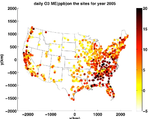
12X12km2 grid cell resolution. ... 60 Figure A. 4s: The DM8A O3 mean prediction error (ME) (in ppb) at each AQS
sites for the CAMx simulation of year 2005 using a 36x36km2 grid cell resolution. ... 60 Figure A. 5s: The DM8A O3 standard deviation of the prediction error (SE)
(in ppb) at each AQS sites for the CAMx simulation of year 2005 using a
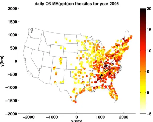
36x36km2 grid cell resolution. ... 61 Figure A. 6s: The DM8A O3 mean prediction error (ME) (in ppb) at each
AQS sites for the CAMx simulation of year 2005 using a 12x12km2 grid cell resolution. ... 61 Figure A. 7s: The DM8A O3 standard deviation of the prediction error (SE) (in ppb)
at each AQS sites for the CAMx simulation of year 2005 using a 12x12km2 grid cell resolution. ... 62 Figure A. 8s: Boxplots of DM8A O3 mean prediction error (ME) and standard
deviation of these prediction error (SE) (in ppb) at AQS sites simulated for year 2005 using the CAMx model simulation with 36x36km2 grid cell resolution, and separated by summer months (May, June, July and August) versus winter months
(November, December, January and February). ... 63
Figure A. 9s: Boxplots of DM8A O3 mean prediction error (ME) and standard deviation of these prediction error (SE) (in ppb) at AQS sites simulated for year 2005 using the CAMx model simulation with 12x12km2 grid cell resolution, and separated by summer months (May, June, July and August) versus winter months
(November, December, January and February). ... 63
Figure A. 10s: Boxplots for the mean prediction errors (ME) and the standard deviation of these prediction errors (SE) of D24A at ozone monitoring sites (888 sites in total) covered by both domains of the CAMx model simulations
with 36x36km2 and 12X12km2 grid cell resolution. ... 64 Figure A. 11s: Boxplots for the mean normalized bias (MNB) and the mean
normalized gross error (MNGE) of D24A at ozone monitoring sites
(888 sites in total) covered by both domains of the CAMx model simulations
with 36x36km2 and 12X12km2 grid cell resolution. ... 64 Figure A. 12s: D24A O3 mean prediction error (ME) (in ppb) at each AQS
sites for the CAMx simulation of year 2005 using a 36x36km2 grid cell resolution. ... 65 Figure A. 13s: D24A O3 standard deviation of the prediction error (SE) (in ppb)
at each AQS sites for the CAMx simulation of year 2005 using a 36x36km2 grid cell resolution. ... 65 Figure A. 14s: D24A O3 mean prediction error (ME) (in ppb) at each AQS sites
xv
Figure A. 15s: D24A O3 standard deviation of the prediction error (SE) (in ppb)
at each AQS sites for the CAMx simulation of year 2005 using a 12x12km2 grid cell resolution. ... 66 Figure A. 16s: Boxplots of D24A O3 mean prediction error (ME) and standard
deviation of these prediction error (SE) (in ppb) at AQS sites simulated for year 2005 using the CAMx model simulation with 36x36km2 grid cell resolution, and separated by summer months (May, June, July and August) versus winter months
(November, December, January and February). ... 67
Figure A. 17s: Boxplots of D24A O3 mean prediction error (ME) and standard deviation of these prediction error (SE) (in ppb) at AQS sites simulated for year 2005 using the CAMx model simulation with 12x12km2 grid cell resolution, and separated by summer months (May, June, July and August) versus winter months
(November, December, January and February). ... 68
Figure A. 18s: The observed DM8A O3 concentrations on the monitoring sites on day 21-July-2005 ... 70
Figure A. 19s: The short range offset for DM8A O3 on the monitoring sites on day 21-July-2005 ... 71
Figure A. 20s: The intermediate range offset for the DM8A O3 on the monitoring
sites on day 21-July-2005 ... 71
Figure A. 21s: The long range offset for the DM8A O3 on the monitoring sites on day 21-July-2005 ... 72
Figure A. 22s: The very long range offset for the DM8A O3 on the monitoring sites
on day 21-July-2005 ... 72
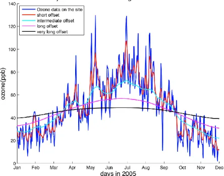
Figure A. 23s: The time series of the DM8A O3 concentrations and four offsets
on a randomly selected site (SiteID:060719004) for year 2005 ... 73
Figure A. 24s: The observed D24A O3 concentrations on the monitoring sites on day 21-July-2005 ... 74
Figure A. 25s: The short range offset for the D24A O3 on the monitoring sites on day 21-July-2005 ... 74
Figure A. 26s: The intermediate range offset for the D24A O3 on the monitoring
sites on day 21-July-2005 ... 75
Figure A. 27s: The long range offset for the D24A O3 on the monitoring sites on day 21-July-2005 ... 75
Figure A. 28s: The very long range offset for the D24A O3 on the monitoring
sites on day 21-July-2005 ... 76
Figure A. 29s: The time series of the D24A O3 concentrations and four offsets
on a randomly selected site (SiteID:060719004) for year 2005 ... 76
Figure A. 30s: Graphs of the 3-structured exponential/exponential covariance models with respect to the spatial lag when the temporal lag is set to 0 (Left)
xvi
Figure A. 31s: Graphs of the 3-structured exponential/exponential covariance models with respect to the spatial lag when the temporal lag is set to 0 (Left)
and with respect to the temporal lag when the spatial lag is set to 0 (Right) for D24A O3 ... 78
Figure A. 32s: Dominance plot showing how the variance changes with respect to the spatial range (Left) and with respect to the temporal range (Right) for
covariance model corresponding to each offset range for DM8A O3 ... 79
Figure A. 33s: Dominance plot showing how the variance changes with respect to the spatial range (Left) and with respect to the temporal range (Right) for
covariance model corresponding to each offset range for D24A O3 ... 79
Figure A. 34s: Maps showing the square root of soft data variance λ2(zi, pi) obtained across the continental United States on 11-July-2005 in (left)
scenario CAMP and (right) scenario RAMP for DM8A O3. ... 80
Figure A. 35s: Maps of BME mean estimates (top panel) and corresponding standard deviations of BME estimates (bottom panel) of the D24A ozone (ppb) on day Jul-21-2005 obtained with scenario OBS (left panels), CAMP
(middle panels) and RAMP (right panels). Circles in the maps represent
locations of monitoring sites and color match legend for observed concentrations. ... 82
Figure A. 36s: D24A O3 concentrations in the United States on 21-July-2005 using (left) the raw CTM Model predictions, (middle) the bias-corrected expected values λ1(zi, pi) for the estimation scenario CAMP, and (right) the bias-corrected
expected values λ1(zi, pi) for the estimation scenario RAMP. ... 84
Figure A. 37s: Maps showing the square root of soft data variance λ2(zi, pi) obtained across the continental United States on 21-July-2005 in (left) scenario
CAMP and (right) scenario RAMP for D24A O3. ... 85
Figure A. 38s: Percent change in mean normalized gross error MNGE shown as a function of cross-validation radius Rv between Scenario RAMP and Scenario OBS. Each curve corresponds to the MNGE calculated using only observations above a given cutoff (0 ppb, 10ppb) of all observations values
for the DM8A O3 (Left) and the D24A O3 (Right). ... 87
Figure A. 39s: Graphs of the 3-structured exponential/exponential covariance functions with respect to the spatial lag (Top panel) and the temporal lag (Bottom panel) for CTM with 36x36km2 cell resolution (Left) and CTM
with 12x12km2 cell resolution (Right) for D24A O3. ... 92 Figure A. 40s: Map of the parameter β0s, t across the continental United
States for day 11-Jul-2005 for the DM8A ozone concentrations ... 94
Figure A. 41s: Map of the parameter β1s, t across the continental United
xvii
Figure A. 42s: Map of the parameter β0s, t across the continental United
States for day 21-Jul-2005 for the D24A ozone concentrations ... 95
Figure A. 43s: Map of the parameter β1s, t across the continental United
States for day 21-Jul-2005 for the D24A ozone concentrations ... 95
Figure B. 1s: Boxplots for the mean prediction errors (ME) and the standard deviation of these prediction errors (SE) of the hourly ozone concentrations at ozone monitoring sites (888 sites in total) covered by both domains of the
CAMx model simulations with 36x36km2 and 12X12km2 grid cell resolution. ... 99 Figure B. 2s: Boxplots for the mean normalized bias (MNB) and the mean
normalized gross error (MNGE) of the hourly ozone concentrations at ozone monitoring sites (888 sites in total) covered by both domains of the CAMx
model simulations with 36x36km2 and 12X12km2 grid cell resolution. ... 99 Figure B. 3s: The hourly O3 mean prediction error (ME) (in ppb) at each AQS
sites for the CAMx simulation of year 2005 using a 36x36km2 grid cell resolution. ... 100 Figure B. 4s: The hourly O3 standard deviation of the prediction error (SE)
(in ppb) at each AQS sites for the CAMx simulation of year 2005 using a
36x36km2 grid cell resolution ... 100 Figure B. 5s: The hourly O3 mean prediction error (ME) (in ppb) at each
AQS sites for the CAMx simulation of year 2005 using a 12x12km2 grid cell resolution. ... 101 Figure B. 6s: The hourly O3 standard deviation of the prediction error (SE)
(in ppb) at each AQS sites for the CAMx simulation of year 2005 using a
12x12km2 grid cell resolution. ... 101 Figure B. 7s: Boxplots for the mean prediction errors (ME) and the standard
deviation of these prediction errors (SE) of the hourly ozone concentrations at ozone monitoring sites for the CAMx model simulations with 36x36km2 grid cell resolution, separated by summer months (May, June, July and August)
versus winter months (November, December, January and February). ... 102
Figure B. 8s: Boxplots for the mean prediction errors (ME) and the standard deviation of these prediction errors (SE) of the hourly ozone concentrations at ozone monitoring sites for the CAMx model simulations with 12x12km2 grid cell resolution, separated by summer months (May, June, July and August)
versus winter months (November, December, January and February). ... 102
Figure B. 9s: Boxplots for the mean normalized bias (MNB) and the mean normalized gross error (MNGE) of the hourly ozone concentrations at ozone monitoring sites for the CAMx model simulations with 36x36km2 grid cell resolution, separated by summer months (May, June, July and August) versus
xviii
Figure B. 10s: Boxplots for the mean normalized bias (MNB) and the mean normalized gross error (MNGE) of the hourly ozone concentrations at ozone monitoring sites for the CAMx model simulations with 12x12km2 grid cell resolution, separated by summer months (May, June, July and August) versus
winter months (November, December, January and February). ... 103
Figure B. 11s: The observed hourly O3 concentrations on the monitoring sites
for UTC hour 20050711T000000 ... 106
Figure B. 12s: The short range offset for hourly O3 on the monitoring sites for
UTC hour 20050711T000000 ... 106
Figure B. 13s: The intermediate range offset for hourly O3 on the monitoring sites
for UTC hour 20050711T00000 ... 107
Figure B. 14s: The long range offset for hourly O3 on the monitoring sites for
UTC hour 20050711T000000 ... 107
Figure B. 15s: The very long range offset for hourly O3 on the monitoring sites for
UTC hour 20050711T000000 ... 108
Figure B. 16s: The time series of the hourly O3 concentrations and four offsets
on a randomly selected site (SiteID:481130069) for year 2005 ... 108
Figure B. 17s: Graphs of the 3-structured exponential/exponential/cosine covariance models with respect to the spatial lag when the temporal lag is set to
0 (Left) and with respect to the temporal lag when the spatial lag is set to 0 (Right) for hourly O3 ... 109
Figure B. 18s: Dominance plot showing how the variance changes with respect to the spatial range (Left) and with respect to the temporal range
(Right) for covariance model corresponding to each offset range for hourly O3 ... 110
Figure B. 19s: Maps of scenario OBS BME mean estimates of the DM8A (Top) and the D24A (Bottom) ozone concentrations (ppb) on day Jul-11-2005 obtained from upscaling method USM1 (Left) and USM2 (Middle), and the
absolute differences between these two methods (Right). ... 111
Figure B. 20s: Maps of R2 (Left) and RMSE (Right) changes for validation analysis conducted with two sets of soft data, one from CTM with 36x36km2 and the other from CTM with 12x12km2 grid cell resolution for D24A at validation radius Rv=0km. Red color in the maps means R2 and RMSE increase when change
the soft data from 36x36km2 to 12x12km2, while blue color means R2 and RMSE decrease. ... 113 Figure B. 21s: Maps of R2 (Left) and RMSE (Right) changes for validation
analysis conducted with two sets of soft data, one from CTM with 36x36km2 and the other from CTM with 12x12km2 grid cell resolution for DM8A at validation radius Rv=0km. Red color in the maps means R2 and RMSE increase when change
xix
Figure C. 1: The time series plot showing the BME mean estimates on simulated
ID18 and the hard data in the neighborhood ... 124
Figure C. 2: The time series plot showing the BME mean estimates on simulated
xx
LIST OF ABBREVIATIONS AND SYMBOLS
AQS Air Quality Systems
BME Bayesian Maximum Entropy
CAMx Comprehensive Air Quality Model with extensions
CMAQ Community Multi-scale Air Quality Modeling System
CTM Chemical transport models
DM8A Daily maximum 8-hour average
D24A Daily 24-hour average
EPA The U.S. Environmental Protection Agency
G-KB General knowledge base
MAQSIP Multiscale Air Quality Simulation Platform
ME Mean error
MNB Mean Normalized Bias
MNGE Mean Normalized Gross Error
NAAQS National Ambient Air Quality Standards
NOx Nitrogen oxides
PCR2 Percent change in R2
PDF Probability Distribution Function
ppb Parts per billion
O3 Ozone
OAQPS The office of air quality planning and standards
R2 Squared Pearson Correlation Coefficent
xxi
SE Standard deviation of the prediction error
S-KB Site specific knowledge base
S/TRF Space/time random field
km Kilometer
km2 Squared kilometer
UTC Coordinated Universal Time
WHIMS Women’s Health Initiative Memory Study
𝑎𝑟 Spatial offset kernel smoothing range 𝑎𝑡 Temporal offset kernel smoothing range
𝑐̂𝑋 Experimental covariance
𝑐𝑋 Covariance model
𝐸[. ] Stochastic expectation
mX Mean trend function
p=(s,t) p is the prediction point; s is the spatial coordinate and t is time
𝑜𝑍(𝒑) Offset at the prediction point p
𝒑𝑘 Space/time estimation point
𝒑𝑚 Space/time soft data points 𝒑𝑜 Space/time observation points 𝑓𝐺 Prior probability distribution function
𝑓𝐾 BME posterior probability distribution function
𝑓𝑆(𝒙𝑚) Soft data PDF characterizing the offset-removed ozone values 𝒙𝑚 𝜆1(𝑧̃𝑖) Expected value
xxii
r Spatial lag
𝑟𝑣 Validation radius
Temporal lag
𝑥𝑘 Offset-removed ozone values at the estimation points 𝒙𝑚 Offset-removed ozone values at the soft data points 𝒙𝑜 Offset-removed hard data at the observational points
𝑧̃𝑗 Ozone CTM model predictions
1
CHAPTER 1 – INTRODUCTION
Ozone is one of the six “criteria” pollutants with established standards in the Clean Air Act
charged by the U.S. Environmental Protection Agency (EPA). The National Ambient Air Quality
Standards (NAAQS) for ozone has been updated a couple times in the history. The current ozone standard
requires that annual fourth-highest daily maximum 8-hour ozone concentrations, averaged over 3 years,
should be less than 70 ppb (parts per billion). Tropospheric ozone has been associated with a wide range
of adverse health outcomes including respiratory effects, cardiovascular effects, central nervous systems
effects and mortality[1].
Most of the evidence on health effects of ozone relates to short-term exposure. The accumulated
evidences on impacts in populations residing in areas with elevated ozone levels for prolonged periods are
more difficult to be detected and are highly uncertain. The Women’s Health Initiative (WHI) memory
study (WHIMS), which involved a nationwide, multicenter cohort of older women aged 65 to 80 years old,
aims to investigate the neurodegenerative effects of long-term ozone exposures in older women. This
large scale cohort study lasted for over 10 years, from year 1996 to year 2006. Our work is to support an
exposure model used to estimate personal exposures of these participants, who came from multiple
metropolitan or rural areas across the continental United States. Spatial and temporal variability in ozone
concentrations vary across different geographical regions and local urban sectors, this has been a major
contributor to the uncertainties in air pollution epidemiologic studies. To achieve the goal of
understanding the adverse health effects of long-term exposure to ozone, accurate ambient estimates of the
2 1.1 Ozone estimates for epidemiologic studies
Epidemiologic studies investigate the associations between health effects and exposure of human
populations to ambient air pollution. These studies fall into several categories, including cross-sectional,
cohort, panel and time-series studies. Despite the epidemiologic study design, the investigator usually
needs to collect data in regards to air pollution exposure level for the study participants or population and
their health outcomes. Exposure measurement error, which is the uncertainty associated with the exposure
metrics used to represent exposure of an individual or population, is an important contributor to
uncertainty in air pollution epidemiologic study results. Exposure error can influence observed
epidemiologic associations between ambient pollutant concentrations and health outcomes by biasing
effect estimates toward or away from the true associations and widening confidence intervals. The
difference between true and estimated exposure to ambient pollutants has been one of the major
components that contribute to exposure measurement error in air pollution epidemiologic studies. Spatial
and temporal variability in ozone concentrations can contribute to exposure error in epidemiologic studies,
especially for cross-sectional and large-scale cohort studies, if the ambient ozone concentrations measured
at the central site monitor is used as an ambient exposure surrogate, which is often different from the
actual ambient ozone concentrations outside a participant’s or a population’s residence. Community
exposure using the ambient ozone measurements at nearby monitoring stations may not be well
represented when monitors cover large areas with several sub-communities having different emission
sources and topographies, such as in Los Angeles, California, where ozone monitors are found to have a
much wider range of inter-monitor correlations (-0.06 to 0.97) than the ones in Atlanta, Georgia (0.61 to
3
Ozone epidemiologic studies use different exposure metrics and have different sources of exposure
error. For ozone short-term exposure, different studies report different daily metrics, including the
maximum 8-hour running average of the hourly concentrations occurring in a 24-hour period (8-hour daily
max)[2-4], the maximum hourly concentrations occurring in a 24-hour period (1-hour daily max)[5, 6] and
the average of the hourly concentrations occurring in a 24-hour period (24-hour average)[7, 8]. According
to the observed ozone concentrations at monitoring sites, the correlations among these common daily
metrics vary site by site. Overall, the two daily peak values, daily 1-hour maximum and daily 8-hour
maximum, are well correlated, with a median correlation of 0.97 across the AQS sites. The correlation
between the 8-hour maximum and 24-hour average are somewhat less well correlated with a median
correlation of 0.89[1]. This indicates the influence of the overnight period on the 24-hour average ozone
concentrations. In contrast, the 1-hour daily max and 8-hour daily max are more indicative of the daytime
ozone concentrations. Little consensus exists as to which metric is the most appropriate. Preferably,
epidemiologic studies are recommended to report results using multiple metrics. For ozone long-term
exposure, a long-term arithmetic mean, such as monthly, quarterly or yearly averages of the above daily
metrics is often computed for the exposure assessment. It is important to recognize the different averaging
times to interpret the health effect estimates reported in epidemiologic studies.
Epidemiologic studies use a wide variety of methods to assign exposure. The commonly used
exposure assessment methods, from simple indicators to complex models, include exposure indicators,
personal monitoring, dispersion modeling, land-use regression modeling and geo-statistical spatial
interpolation methods. Each method has its advantages and disadvantages when applied to individual
studies. For example, personal monitoring has the advantage of providing relatively accurate
individual-level exposure data, but the disadvantage is that it is very costly and time consuming so it is only practical
in small scale studies involving a limited number of participants. The major disadvantage of dispersion
modeling is that it requires highly specific input data, including specific emission inventories and
4
Among different geo-statistical methods, the four commonly used methods are spatial averaging,
nearest neighbor, inverse distance weighting and kriging. All of these four methods are weighted average
methods, with the interpolation process involving the following steps: 1) defining the search area or
neighborhood around the point of interest; 2) locating the observed data points within this neighborhood;
and 3) assigning appropriate weights to each of the observed data points. The differences are in their
choices of sample weights. With spatial averaging, the same fractional weights are assigned to all sampled
values within a fixed distance. With nearest neighbor method, only a single sampled value is used and a
weight of 1 is assigned. With inverse distance weighting, the closer samples are assigned with larger
weights. With kriging, the weights are assigned based on the spatial autocorrelation statistics of the
sampled dataset. The common limitation of these interpolation methods is that it relies on the
observational data alone, which poses a bigger challenge for those areas where the monitoring stations are
very sparse and/or those time periods where ozone monitoring data is missing.
1.2 Environmental sources of ozone data
An important environmental source of ozone data is measurements from routine monitoring
networks. In the United States, EPA regulations require state environmental agencies to operate air
pollution monitoring stations and report air monitoring data to the Air Quality System (AQS) database,
which is a repository of the monitoring data collected across various monitoring networks. The hourly
ozone observational data from these monitoring stations are available from year 1993 to the present. The
office of air quality planning and standards (OAQPS) rely upon ozone measurements for air quality
assessment and attainment/non-attainment designations. By year 2015, there are over 1250 ozone monitors
reporting hourly data to AQS. Strict quality assurance and quality control procedures for ozone
monitoring have been developed and implemented at the monitoring stations. The hourly ozone
concentrations reported to the AQS database can be considered as a reliable and accurate data source.
There are, however, some limitations in this data source. The distribution of ozone monitors across urban
5
depend on many factors, such as the magnitude of the concentrations and population density. The densest
ozone monitoring sites are located in California and the eastern U.S, while relatively scarce across the
central U.S. Further, the monitoring durations on the stations are not consistent. Due to the strong
seasonality of ozone concentrations, many states limit their ozone monitoring to a certain portion of the
year, termed the ozone season, the length of which varies from one area of the country to another. As a
result, less than half of the ozone monitoring sites in the U.S. operate year-round. The majority of the
sites only operate for summer months. This is why the estimation approaches solely based on
observational data in many of the previous epidemiological studies suffer from the missing data issues due
to the sparse monitoring network across space and the inconsistent monitoring durations.
Besides ozone monitoring networks, numerical model predictions have become a second source of
environmental ozone data. For more than a decade, air quality models such as Community Multi-scale Air
Quality Modeling System (CMAQ) and Comprehensive Air Quality Model with extensions (CAMx) have
been used as powerful computational tools for air quality management. These models unite three major
types of models, including meteorological models, emission models and a chemistry-transport model.
They are designed to approach air quality as a whole by including state-of-science capabilities for
modeling multiple air quality issues. These models can simulate air pollution concentrations as averaged
values of grid cells with continuous spatial and temporal coverage. For the purpose of air quality
management and evaluation in the United States, there has been a wide range of modeling simulations
completed which cover various model configurations, domains, episodes, chemical mechanisms and
aerosol modules[9-14]. The acceptability of these models’ performance was judged by comparisons of the
model predicted concentrations, usually the daily 8-hour maximum ozone, to the corresponding observed
values at monitoring sites. The modeling community has made significant progress in reducing the
emission uncertainties and inaccuracy of the chemical mechanisms in the air quality models to reduce the
prediction errors. Ozone model performance has been slowly improved as these modeling systems
advance. Overall, the daily 8-hour maximum ozone performance at AQS monitoring sites are relatively
6
less than 20%. Although these models still have inherent uncertainties and weakness, the ozone
concentrations predicted by these modeling platforms can closely reflect the corresponding observed
concentrations in space and time. Our work is to take what is available and make use of them.
Due to limited computational resources, CTM model applications on national scale usually use a
coarser horizontal grid cell resolution, such as 36x36 km2 for Continental U.S. or 12x12 km2 for the eastern U.S. covering thirty seven eastern states. Model predictions from the 36x36 km2 Continental U.S. domain were often used to provide initial and boundary concentrations for simulations in the 12x12 km2 domain. For those applications studying air quality at local scale, finer horizontal grid cell resolutions,
such as 4x4 km2 or 2x2 km2 have been used. In theory, higher resolution modeling is expected to yield better predictions because of better resolved model input fields, such as topography, land cover or
emissions, and better mathematical characterization of physical and chemical processes. Ozone model
performance dependence on grid resolution have been examined [15, 16]. In general, finer grid scales are
found to be able to better resolve the local scale spatial variability of ozone concentrations. The newest
release CMAQ 5.1 enables improved fine-scale simulations allowing users to simulate air quality at
smaller settings like metropolitan areas as fine as 1x1km2 grid cell resolution. Improvements in
computational efficiency are expected to enable higher resolution in the future release of these modeling
system.
1.3 Geo-statistical approaches for integration of environmental data from multiple sources
Geo-statistical approaches provide useful solution to integrate air pollution measurements and
other relevant information. Several Bayesian inference approaches [17-19] have been developed to
provide a sophisticated statistical framework for the data integration of observations and CTM model
predictions to improve ambient air pollution exposure estimates. These approaches share the following
characteristics: parameterize the relationship between air pollution observations and predictions, using
kriging to obtain air pollution estimates for any given value of the parameters, and use Bayesian inference
7
following limitations: they assume that the relationship between air pollution observations and predictions
is linear and homoscedastic, they share the linear limitations of the kriging estimator, and require a high
computational cost.
One approach is the Bayesian Maximum Entropy (BME) method of modern geo-statistics, a
knowledge-processing framework, because of its following advantages. First of all, it can incorporate
different kinds of knowledge bases, such as general knowledge derived from physical laws, scientific
theories and specific knowledge processed from a given situation. Secondly, there are no assumptions
about the shape and distribution of the underlying probability law. Therefore, it can integrate a wide
variety of nonlinear, non-Gaussian uncertain datasets in a probabilistic way. Thirdly, it is computational
effective in spatial and temporal domains.
In the past few years, BME has been applied to map criteria pollutant [20, 21]. Using BME to
integrate air monitoring observations and numerical model predictions has been proven to be a
cost-effective and efficient technique in improving spatial predictions of ozone concentrations. It allows us to
take advantage of the strength from both data sources, the accuracy of the observational data and the good
spatial/temporal coverage of air quality model outputs without assuming a parametric relationship between
these two data sources. In de Nazelle et al. [20], BME framework was used to develop ozone estimates for
the state of North Carolina for a short study period, June 19th to June 30th of year 1996. The observational
data from the state’s ozone monitoring network in combination with model outputs from the Multiscale
Air Quality Simulation Platform (MAQSIP) modeling system were integrated. In this study, the BME
framework gave preference to measured ozone data, also used MAQSIP model outputs as a function of
model performance. It showed that the BME data integration approach improves the accuracy and the
precision of ozone estimations across the state of North Carolina when compared to a spatial interpolation
8 1.4 Thesis Hypothesis and approach
Our hypothesis is that fully characterizing the spatial and temporal heterogeneity in CTM model
performance in our geo-statistical approach can increase estimation accuracy. In de Nazelle’s work [20],
air quality model performance was assumed to be homogeneous for the study domain, so the bias and
uncertainty associated with the model predictions were assumed to be the same across space and time.
Therefore, the soft data was processed through pooling all the paired observed and modeled ozone
concentrations in the domain at one time. This assumption might be reasonable given the small study
domain and short study period, but may not be applicable due to the documented spatial heterogeneity and
temporal variability of ozone model performance across the country. Therefore, we need to extend the
work of de Nazelle et. al’s by developing a new approach that can accommodate the spatial or seasonal
variability in the ozone model performance of the CTM.
To test this hypothesis, we describe in Chapter 2 the development of a Regionalized Air Quality
Model Performance (RAMP) approach to characterize the ozone model prediction errors that changes
across space/time. Instead of making the assumption of air quality model performance homogeneity, we
generate soft data as secondary information, to reflect the bias and uncertainty of model predictions
changing across space and time. As a result, the RAMP approach is expected to capture geographical and
temporal changes in bias and uncertainty associated with air quality model predictions. The soft data
generated from RAMP approach is integrated with the ozone observations in our BME model framework
to produce ozone estimates. We first compare the RAMP estimation with two other estimation scenarios,
one using only ozone observations, and the other is a Constant Air Quality Model Performance (CAMP)
scenario assuming that CTM model performance does not change across space and time. We also compare
our BME estimation to a cokriging estimation based on a parametric relationship between the observations
9
For the WHIMS work, the BME approach was used to interpolate directly the daily ozone
concentrations by first aggregating the hourly observations and CTM model predictions. An alternative
approach would be to first generate hourly BME estimates then aggregate it into a daily metrics. This
alternative approach could be especially useful for those epidemiologic studies that require higher
temporal resolution of ambient exposure estimates, such as those exposure models combining
microenvironmental concentrations with human activity data to estimate personal exposures. This could
be relevant given the known diurnal patterns seen in hourly ozone data. The disadvantage of this
alternative approach is the computational intensity, requiring over 200 times more CPU runtime. In
Chapter 3, our first task was to investigate the extent of the improvement on the accuracy of the hourly
ozone estimates when incorporating CTM hourly model predictions through our RAMP approach. Our
second task is to investigate the differences of the predictive capacity between these two choices of
generating daily ozone estimates. We conducted a comparison of two upscaling methods: USM1 (data
aggregation from hourly to daily followed by BME approach estimation) and USM2 (perform BME
approach estimation on hourly ozone followed by data aggregation). A validation analysis using only
non-collocated data outside of a validation radius was performed and the error statistics between the
observations and re-estimated values for two daily metrics, the daily maximum 8-hour average (DM8A)
and the daily 24-hour average (D24A) ozone concentrations, were obtained to investigate the estimation
10
CHAPTER 2 – BAYESIAN MAXIMUM ENTROPY INTEGRATION OF OZONE
OBSERVATIONS AND MODEL PREDICTIONS: A NATIONAL APPLICATION1
2.1 Introduction
According to EPA’s newly released Integrated Science Assessment for tropospheric ozone[1], the
evidence of public health impacts on populations residing in areas with elevated ozone levels for
prolonged periods are still uncertain. A better understanding of the adverse health effects to chronic ozone
requires accurate exposure estimates at multiple temporal scales and at fine spatial resolutions. Estimates
of ozone concentrations typically rely on environmental data collected from two sources: monitoring
networks and air quality chemical transport models (CTM). The first source gives measurement
concentrations for a long temporal time, but only at a point where the monitor is located. The CTM
provides predictions for all locations, but is an average concentration based on the spatial resolution of the
model grid cell. Further, given the intensive resources needed to build a CTM, the numbers of days that are
simulated are limited. Several categories of data integration methods, including Kalman filter methods[22],
variational methods [23], optimal interpolation [24] and Bayesian methods [17-19] have been developed to
integrate these two types of data and rely on their individual strengths to build a more refined air pollution
estimate. In this work, we choose the BME method of modern geostatistics, a knowledge-processing
framework, because of its advantage of integrating a wide variety of nonlinear, non-Gaussian knowledge
bases.
11
We developed our data integration approach to obtain two metrics of ozone estimates, the DM8A
and D24A ozone concentrations. Both of these metrics are commonly used in epidemiology studies [7, 8,
25].
Several Bayesian inference approaches [17-19] provide a sophisticated statistical framework for
the data integration of ozone observations and model predictions and production of multiple time averaged
estimates. These approaches share the following characteristics: parameterize the relationship between air
pollution observations and predictions, use kriging to obtain air pollution estimates for any given value of
the parameters, and use Bayesian inference to obtain air pollution estimates that accounts for parameter
uncertainty. These methods, however, have the following limitations: they assume that the relationship
between air pollution observations and predictions is linear and homoscedastic, they share the linear
limitations of the kriging estimator, and have a high numerical cost.
To overcome these limitations de Nazelle et al. [20] introduced an approach based on the nonlinear
extension of kriging provided by the Bayesian Maximum Entropy (BME) method of modern
spatiotemporal geostatistics[26]. This approach uses a non-parametric methodology that fully accounts for
the non-linearity and non-homoscedasticity of the relationship between air pollution observations and
predictions. Their application of this approach showed that the BME method provided a numerically
efficient data integration framework that combines a wide variety of nonlinear, non-Gaussian knowledge
bases that are out of the reach of kriging-based methods. That study applied the BME framework to
integrate ozone observations and model predictions simulated by the Multiscale Air Quality Simulation
Platform (MAQSIP) in the state of North Carolina and exposure were estimated for a short study period,
June 19th to June 30th of year 1996. That study demonstrated that the BME data integration approach, by incorporating the MAQSIP model predictions along with ozone observations, improved both the accuracy
12
It is clear from the de Nazelle et al.’s work that the authors assumed that the model performance
from the air quality model for ozone was homogeneous for the entire state. This was a reasonable
assumption given the small study domain and short study period. In our work here, however, we are
providing ozone estimates for the entire continental United States (US) for multiple time averages that
could include a full year. Thus, de Nazelle et al’s assumption may not be applicable due to the unknown
spatial heterogeneity and temporal variability of ozone model performance across the country. Therefore,
we extend the work of de Nazelle et al’s by developing our new RAMP approach that can accommodate
any spatial or seasonal variability in the model performance of the CTM. The refined ozone estimates that
we obtain could be applied for health assessments or adapted to generate exposure estimates for other
criteria air pollutants.
2.2 Data
2.2.1 Ozone Monitoring Data
The DM8A and D24A ozone concentrations for each monitoring site and day for the year 2005
were constructed based on raw monitoring data from ozone monitoring stations measuring hourly O3
concentrations using the procedure described here.
We downloaded hourly ozone monitoring data (raw data) sampled from 1179 sites in the Air
Quality Systems (AQS) database maintained by the U.S. Environmental Protection Agency (EPA), which
is a repository of the monitoring data collected across various monitoring networks. Then we computed the
DM8A and D24A of hourly ozone concentrations at each monitoring site to construct a daily ozone
concentration database. These daily averages are considered as hard data, an error-free proxy, in our later
13 2.2.2 Air Quality Model Predictions
The air quality model data consists of hourly ozone concentrations predicted by the
Comprehensive Air Quality Model with extensions (CAMx)[27] modeling system on a 36x36km2 grid cell
resolution domain covering the continental U.S. and a 12x12km2 grid cell resolution domain covering the
Eastern U.S. as shown in Figure 1s. CAMx is a publicly available Eulerian grid-based model that can
address tropospheric ozone, acid deposition, visibility, fine particulates and other air pollutants issues in
the context of a “one atmosphere” perspective. The modeling simulations were created by the U.S. EPA as
base-case simulations in their analysis of the final Transport Rule. These air quality-modeling simulations
used the CAMx version v5.30 with gas-phase chemistry mechanism CB05, and also refined
meteorological and emission fields for the year 2005 across the United States. Detailed model
configurations and evaluation are discussed elsewhere[28].The hourly model predictions were used to
compute the DM8A and D24A ozone concentrations at each grid cell. These CTM predicted daily ozone
concentrations are used to construct the soft data, as secondary information with uncertainties, consisting
of the expected values of the daily concentrations and the uncertainties associated with the expected values
at each grid cell. The details of soft data construction are described in section 3.3.
2.3 Methods
2.3.1 BME Estimation Methodology
BME is a modern geo-statistical method [26] for spatial-temporal interpolation that incorporates
information from many different data sources. The implementation and performance of BME have been
detailed in other works[21, 29], and its application to the integration of O3 observations and model
predictions was described by de Nazelle et al[20]. In short, we model the (offset-removed) transform,
which is a commonly used deterministic transformation[30], of air pollution as a Space/Time Random
Field (S/TRF) X(p) at space/time coordinate p=(s,t), where s is the spatial coordinate and t is time. Our
notation for S/TRFs consists of denoting a single random variable 𝑋in capital letters, its realization, 𝑥, in
14
characterizing X(p) consists of the mean function 𝑚𝑋(𝒑) = 𝐸[𝑋], where 𝐸[. ] is the stochastic expectation, describing its consistent trends, and the covariance function 𝑐𝑋(𝒑, 𝒑′) = 𝐸[(𝑋(𝒑) − 𝑚(𝒑)(𝑋(𝒑′) − 𝑚(𝒑′))] describing its space/time dependencies. Likewise the site specific knowledge base (S-KB) consists of the hard data 𝒙𝑜 at space/time observation points 𝒑𝑜 located at the monitoring stations, and the soft data charactering the S/TRF values 𝒙𝑚 at the space/time model prediction points 𝒑𝑚 in terms of a site-specific PDF 𝑓𝑆(𝒙𝑚). Denoting the G-KB as 𝐺 = {𝑚𝑋(𝒑), 𝑐𝑋(𝒑, 𝒑′)} and the S-KB as 𝑆 = {𝒙𝑜 , 𝑓𝑠(𝒙𝑚)},
we can summarize the BME steps as 1) using the Maximum Entropy principle of information theory to
process the G-KB in the form of a prior Probability Distribution Function (PDF) 𝑓𝐺, 2) integrating the
S-KB using an epistemic Bayesian conditionalization rule to create a BME posterior PDF 𝑓𝐾 characterizing the value 𝑥𝑘 taken by X(p) at any estimation point 𝒑𝑘 of interest, and 3) computing space/time estimates
based on the BME posterior PDF. The BME posterior PDF is given by the BME equation
𝑓𝐾(𝑥𝑘) = 𝐴−1∫ 𝑑𝒙𝑚 𝑓𝑆(𝒙𝑚)𝑓𝐺(𝒙𝑚𝑎𝑝) (E2-1) where 𝒙𝑚𝑎𝑝 = (𝑥𝑘, 𝒙𝑜, 𝒙𝑚) is the value of 𝑋(𝒑) at points 𝒑𝑚𝑎𝑝= (𝒑𝑘, 𝒑𝑜, 𝒑𝑚) and 𝐴 is a normalization
constant.
Let 𝑍(𝒑) = 𝑍(𝒔, 𝑡) be the Space/Time Random Field (S/TRF) representing daily ozone. In this study
we define 𝑍(𝒔, 𝑡) as the sum of a homogenous/stationary S/TRF and a known offset as follows. We first
define the transformation of the ozone observational data 𝒛𝑜 at locations po as
𝒙𝑜= 𝒛𝑜– 𝑜𝑍(𝒑𝑜) (E2-2) where 𝑜𝑍(𝒑) may be any deterministic offset that can be mathematically calculated without error as a
function of the space/time coordinate p. We then define 𝑋(𝒑) as a homogeneous/stationary S/TRF
15
The soft data are described by the PDF 𝑓𝑆(𝒙𝑚) characterizing the offset-removed ozone values 𝒙𝑚 at the soft data points 𝒑𝑚 corresponding to the centroids of the nm CTM computational nodes. The
offset-removed ozone model predictions 𝑥̃𝑖 are calculated at these nodes. As a key conceptual aspect of our work,
the generation of this soft data PDF requires not only the offset-removed ozone model predictions, but also
the observation-prediction pairs where the observed and CTM predicted ozone concentrations are paired
across space and time. This PDF is expressed as
𝑓𝑆(𝒙m) = ∏𝑛𝑖𝑚𝑓(𝑥𝑖|𝑥̃𝑖, 𝒑𝑖) (E2-3) which essentially characterizes how well each CTM offset-removed ozone value 𝑥̃𝑖 predicts the true offset-removed ozone concentration 𝑥𝑖 at the computational prediction point 𝒑𝑖. Procedurally equation (3) is simply obtained by first calculating 𝑓𝑆(𝐳𝐬) = ∏𝑖𝑛𝑚𝑓(𝑧𝑖|𝑧̃𝑖, 𝒑𝑖), where 𝑧𝑖 and 𝑧̃𝑖 are observed and CTM predicted ozone values, respectively, and then using the offset relationship 𝒙𝑠= 𝒛𝑠– 𝑜𝑍(𝒑𝑠) to obtain 𝑓𝑆(𝒙𝐬).
As described by de Nazelle et al [31], the PDF 𝑓(𝑧𝑖|𝑧̃𝑖, 𝒑𝑖) is modeled using a parameterized
statistical distribution, chosen to be the normal distribution truncated below zero with an expected value
𝜆1(𝑧̃𝑖) and variance 𝜆2(𝑧̃𝑖), such that:
𝑓(𝑧𝑖|𝑧̃𝑖) = Φ( 𝑧𝑖; 𝜆1(𝑧̃𝑖), 𝜆2(𝑧̃𝑖)) (E2-4) In the soft data construction approach implemented by de Nazelle et al [31] the parameters 𝜆1(𝑧̃𝑖) and 𝜆2(𝑧̃𝑖) vary as a function of the model prediction 𝑧̃𝑖 but are constant with respect to the space/time point 𝒑𝑖, hence their implementation is based on a Constant Air quality Model Performance (CAMP). The
CAMP approach was appropriate since in their application the air quality model performance did not
16
Our aim, however, is to extend the BME methodological framework to the national domain by modeling
𝜆1(𝑧̃𝑖, 𝒑𝑖) and 𝜆2(𝑧̃𝑖, 𝒑𝑖) as a function of both 𝑧̃𝑖 and the space and time coordinate 𝒑𝑖, expressed as below. 𝑓(𝑧𝑖|𝑧̃𝑖, 𝒑𝑖) = Φ( 𝑧𝑖; 𝜆1(𝑧̃𝑖, 𝒑𝑖), 𝜆2(𝑧̃𝑖, 𝒑𝑖)) (E2-5)
Therefore, we need to investigate how the air quality model performance varies across the continental US.
2.3.2 Variability of CTM Model Performance Evaluation across the Continental US
Each observed daily concentration 𝑧𝑗 is paired with its corresponding CTM prediction value 𝑧̃𝑗, and the error for the observation-prediction pair is defined as 𝑒𝑗 = 𝑧̃𝑗− 𝑧𝑗. To evaluate the air quality
model performance over a given space time region R of interest, we calculate error statistics such as the
Mean prediction Error (ME), the Standard deviation of the prediction Error (SE), the mean normalized bias
(MNB) and the mean normalized gross error (MNGE) as defined in SI equations A.1s-A.4s.
According to the model performance analysis of this CTM (see Supporting Information (SI)
section A.1), for the DM8A O3, we find that overall the CAMx simulation with 12x12km2 grid cell
resolution has a substantially lower over-prediction (median ME=+1.4ppb) than that with 36x36km2 grid
cell resolution (median ME=+4.5 ppb). Furthermore, as summarized in Figures A.2s and A.3s, the ME,
SE, MNB and MNGE at individual monitoring sites vary over a wider range for the simulation with
36x36km2 grid cell resolution. The variability of these ME and SE values exhibit clear geographical trends
(SI figures A.4s-7s for the DM8A and figures A.12s-15s for the D24A): Urban cities located in the east
and west coast tend to have higher over-prediction bias (i.e. higher ME) and higher imprecision (i.e. higher
SE) than sites located in the central United States. We also found noticeable seasonal differences in the
model performance for both CTM simulations (SI Figures A.8s-9s for the DM8A and figures A.16s-17s
17
The results of this analysis provide strong evidence that the performance of CTM varies
considerably across the national domain and over seasons. Therefore, there is a need to extend the
implementation of the BME framework to account for this space/time variability in model performance.
We use the Regionalized Air Quality Model Performance (RAMP) method to quantify how the expected
value 𝜆1(𝑧̃𝑖, 𝒑𝑖) and variance 𝜆2(𝑧̃𝑖, 𝒑𝑖) for the ozone soft data derived from CTM outputs vary as a function of both the CTM prediction 𝑧̃𝑖 and the space/time computational node 𝒑𝑖 for which that prediction
was calculated. The goal of the RAMP method is to select the most relevant observation-prediction pairs to
most accurately identify the CTM bias associated with the prediction value 𝑧̃𝑖 outputted for any space/time computational node 𝒑𝑖 of interest.
2.3.3 The Proposed Regionalized Air Quality Model Performance (RAMP) Evaluation Framework
In the first stage of the RAMP analysis, we pool for each monitoring site the
observation-prediction pairs (𝑧𝑗, 𝑧̃𝑗) that are within a time tolerance of 𝛥𝑇 = 120 𝑑𝑎𝑦𝑠 of a particular time of interest t. Examples of two selected sites are shown in Figure 1. These pairs are highly relevant to the location 𝒔𝑛 where the monitoring station is sited, and the 120 days time window is chosen to balance the abundance of
the pairs and the intention to retain seasonal specificity in the 𝑧̃𝑗− 𝑧𝑗 differences. We stratify the pairs in 10 equal percentile bins of increasing predicted values 𝑧̃𝑗, and for each bin we calculate the mean and
variance of observed values,
𝜆̂1(𝑧̃𝑏, 𝒔𝑛, 𝑡) = 1
𝑛0(𝑧̃𝑏,𝒔𝑛,𝑡)∑ 𝑧𝑗 𝑛0(𝑧̃𝑏,𝒔𝑛,𝑡)
𝑗=1 (E2-6) 𝜆̂2(𝑧̃𝑏, 𝒔𝑛, 𝑡) = 1
𝑛0(𝑧̃𝑏,𝒔𝑛,𝑡)∑ (𝑧𝑗− 𝜆̂1(𝑧̃𝑏, 𝒔𝑛, 𝑡)) 2 𝑛0(𝑧̃𝑏,𝒔𝑛,𝑡)
𝑗=1 (E2-7) where 𝑛0(𝑧̃𝑏, 𝒔𝑛, 𝑡) is the number of (𝑧𝑗, 𝑧̃𝑗) pairs in the bth bin, 𝑧
18
Figure 2. 1: RAMP analysis conducted specifically at time t=11-Jul-2005 and for sites ID 060372005(left) and 120713002(right). The empty circles show the pairs of observed-modeled values (𝑧𝑗, 𝑧̃𝑗) that are within 120 days of t. The vertical lines show the stratification of these pairs in 10 bins. The interpolation lines connecting the filled circles and triangles show how the mean of the observed value in each bin,
𝜆̂1(𝑧̃𝑏, 𝒔𝑛, 𝑡) (filled circles), and the corresponding standard deviation, √𝜆̂2(𝑧̃𝑏, 𝒔𝑛, 𝑡) (filled triangles) change as a function of the average modeled value 𝑧̃𝑏 in that bin.
In the second stage of the RAMP analysis we obtain 𝜆1(𝑧̃𝑖, 𝒑𝑖) and 𝜆2(𝑧̃𝑖, 𝒑𝑖) for actual predicted values 𝑧̃𝑖 and space/time grid point 𝒑𝑖 = (𝒔𝑖, 𝑡𝑖) as follows. For each monitoring site 𝒔𝑛 we perform a linear interpolation/extrapolation of the 𝜆̂1(𝑧̃𝑏, 𝒔𝑛, 𝑡𝑖) and 𝜆̂2(𝑧̃𝑏, 𝒔𝑛, 𝑡𝑖) values to obtain 𝜆1(𝑧̃𝑖, 𝒔𝑛, 𝑡𝑖) and 𝜆̂2(𝑧̃𝑖, 𝒔𝑛, 𝑡𝑖) (see interpolation lines in figure 3), and then we do a spatial interpolation of these values to obtain 𝜆̂1(𝑧̃𝑖, 𝒑𝑖) and 𝜆̂2(𝑧̃𝑖, 𝒑𝑖) at 𝒑𝑖 = (𝒔𝑖, 𝑡𝑖) using the following formula
𝜆̂1 𝑜𝑟 2(𝑧̃𝑖, 𝒔𝑖, 𝑡𝑖) =∑ 𝑤𝑖 𝑁
𝑛=1 (𝒔𝑖,𝒔𝑛)𝜆̂1 𝑜𝑟 2(𝑧̃𝑖,𝒔𝑛,𝑡𝑖)
∑𝑁𝑛=1𝑤𝑖(𝒔𝑖,𝒔𝑛) ; 𝑤𝑖(𝒔𝑖, 𝒔𝑛) = 1
𝑑𝑖𝑠𝑡(𝒔𝑖,𝒔𝑛) (E2-8) where n=1,…N refers the N monitoring sites closest to the location of the computational node 𝒔𝑖 of
interest, and 𝑤𝑖(𝒔𝑖, 𝒔𝑛) is a weight equal to the inverse of the distance between the computational node 𝒔𝑖
of interest and the n-th neighboring monitoring station.
Stated simply 𝑧̃𝑖− 𝜆̂1(𝑧̃𝑖, 𝒑𝑖) is the bias characterizing systematic errors associated with a CTM prediction value of 𝑧̃𝑖 calculated at space/time grid point 𝒑𝑖= (𝒔𝑖, 𝑡𝑖), and 𝜆̂2(𝑧̃𝑖, 𝒑𝑖) is the variance characterizing the associated imprecision. The strength of the RAMP method is that it does not make any
assumption on the relationship between observed and predicted values, and therefore geographical and