biom.13175.pdf

(1)

Design and analysis of bridging studies with prior probabilities

on the null and alternative hypotheses

Donglin Zeng

1

_{Zhiying Pan}

2

_{D. Y. Lin}

1

1_{Department of Biostatistics, University of}

North Carolina, Chapel Hill, North Carolina

2_{Amgen Inc, 1 Amgen Center Dr, Thousand}

Oaks, California

Correspondence

Donglin Zeng, Department of Biostatistics, University of North Carolina, Chapel Hill, NC 27599-7420.

Email: [email protected]

Funding information

National Institute of General Medical Sciences, Grant/Award Numbers: R01 GM124104, R01 GM047845

Abstract

The pharmaceutical industry and regulatory agencies are increasingly interested in conducting bridging studies in order to bring an approved drug product from the orig-inal region (eg, United States or European Union) to a new region (eg, Asian-Pacific countries). In this article, we provide a new methodology for the design and analy-sis of bridging studies by assuming prior knowledge on how the null and alternative hypotheses in the original, foreign study are related to the null and alternative hypothe-ses in the bridging study and setting the type I error for the bridging study according to the strength of the foreign-study evidence. The new methodology accounts for ran-domness in the foreign-study evidence and controls the average type I error of the bridging study over all possibilities of the foreign-study evidence. In addition, the new methodology increases statistical power, when compared to approaches that do not use foreign-study evidence, and it allows for the possibility of not conducting the bridging study when the foreign-study evidence is unfavorable. Finally, we conducted extensive simulation studies to demonstrate the usefulness of the proposed methodology.

K E Y W O R D S

adaptive significance level, bridging studies, ethnic factors, foreign studies, optimal designs, sample size calculations

1 INTRODUCTION

In an effort to expedite the availability of drug products to dif-ferent populations, regulatory authorities and pharmaceutical companies are increasingly interested in bringing an approved drug product from the original region (eg, United States or European Union) to a new region (eg, Asian-Pacific coun-tries) by utilizing the original clinical trial data to meet the regulatory standards and clinical trial practices of the new region. In 1998, the International Conference on Harmoniza-tion (ICH) issued a guideline, entitled “Ethnic Factors in the Acceptability of Foreign Clinical Data” (known as ICH E5), to provide guidance on regulatory and development strate-gies that will permit adequate evaluation of the influence of ethnic factors on efficacy, safety, dosage, and dose reg-imen, while minimizing duplication of clinical studies and

(2)

Several methods have been developed for the design and analysis of bridging studies; see Chow et al. (2012) for a review. Specifically, Shao and Chow (2002) proposed a sen-sitivity index to assess the reproducibility probability, and Shih (2001) suggested a sequential procedure to test the consistency between the foreign and bridging studies. To design a bridging study, Liuet al. (2002) and Hsiaoet al. (2007) proposed Bayesian methods by assuming normal or mixture-normal priors for the drug effects based on the for-eign study, such that the posterior distribution for the drug effect can be derived after combining data from the two studies. These Bayesian methods require strong distributional assumptions on both the data and priors. Alternatively, Lan et al. (2005), Lan and Pinheiro (2012), and Huang et al. (2012) proposed a weighted statistic that is a weighted sum of the 𝑍-statistics from the foreign and bridging studies. The type I error or power for the bridging study is obtained by conditioning on the evidence from the foreign study and the prespecified weights. Although the statistics from the two studies are usually normalized, a weighted sum of the test statistics is not biologically interpretable. When the two statistics have opposite directions, the weighted sum may lead to lower power than using evidence from the bridging study only.

In this article, we propose a new framework for incor-porating evidence from the foreign study into the design and analysis of the bridging study. In order to leverage the evidence from the foreign study, we assume certain prior probabilities on the relationship between the null and alternative hypotheses in the two studies. We use an adaptive significance level to design the bridging study based on the strength of the evidence in the foreign study. By accounting for the randomness of the foreign-study evidence and the uncertainty of the foreign-study truth, the proposed adaptive significance level for the bridging study guarantees that the overall type I error of the bridging study (ie, averaged over all possible scenarios of the foreign-study evidence) will be controlled at a prespecified level. In addition, we devise a grid-search algorithm to determine the optimal choice of the adaptive significance level that ensures higher power than the bridging study without using evidence from the foreign study.

2 METHODS

We use subscript 1 to denote the foreign study and subscript 2 to denote the bridging study. For𝑘=1 and 2, letΔ_𝑘denote the parameter of interest that quantifies the difference between the test and control groups (eg, the difference or the log-ratio of the response rates) in the𝑘th study. We wish to test the null hypothesis

𝐻_𝑘₀∶ Δ_𝑘∉ (𝐿_𝑘, 𝑈_𝑘)

against the alternative hypothesis

𝐻_𝑘𝑎∶ Δ_𝑘∈ (𝐿_𝑘, 𝑈_𝑘),

where𝐿_𝑘and𝑈_𝑘are specific margins. The constants𝐿_𝑘and 𝑈_𝑘are chosen to yield different types of tests: the equivalence test corresponds to finite𝐿_𝑘 and𝑈_𝑘; superiority test corre-sponds to𝐿_𝑘= 0and𝑈_𝑘= ∞; and the noninferiority test cor-responds to𝐿_𝑘<0and𝑈_𝑘= ∞.

2.1 Priors for hypotheses

The main reason that one can incorporate evidence from the foreign study into the design or analysis of the bridging study for certain drugs is because the drug’s safety, efficacy, dosage, and dose regimen are similar across regions. Intuitively, if the null (or alternative) hypothesis holds for the foreign study, then there is a high likelihood that the null (or correspond-ingly, alternative) hypothesis holds for the bridging study and vice versa. Thus, we wish to weigh the strength of the foreign-study evidence when deciding whether or not to reject𝐻₂₀. Specifically, we consider𝐻₁₀ and𝐻₁_𝑎as random variables whose distributions depend on whether𝐻₂₀or𝐻₂_𝑎holds, and we impose the following assumptions a priori:

Assumption 1. There exists some constant𝑝∈ [0.5,1]such that

Pr(𝐻₁₀|𝐻₂₀) =𝑝.

Assumption 2. There exists some constant𝑞∈ [0,1] such that

Pr(𝐻₁_𝑎|𝐻₂_𝑎) =𝑞.

(3)

conditional on𝐻₂₀or𝐻₂_𝑎. This is a reasonable assumption in practice.

Remark1. Since we are using the foreign study evidence to design and analyze the bridging study, it would seem more natural to considerPr(𝐻₂₀|𝐻₁₀) andPr(𝐻₂_𝑎|𝐻₁_𝑎) rather thanPr(𝐻₁₀|𝐻₂₀) andPr(𝐻₁_𝑎|𝐻₂_𝑎). By Bayes’ theorem; however, we can convertPr(𝐻₁₀|𝐻₂₀)andPr(𝐻₁_𝑎|𝐻₂_𝑎)to Pr(𝐻₂₀|𝐻₁₀)andPr(𝐻₂_𝑎|𝐻₁_𝑎)and vice versa. Because we wish to control the type I error and improve the power for the bridging study, we are primarily interested in the rejection probabilities conditional on the null or alternative hypothe-sis in the bridging study. Specifically, we need to evaluate Pr(𝐻₁₀|𝐻₂₀) andPr(𝐻₁_𝑎|𝐻₂_𝑎) rather than Pr(𝐻₂₀|𝐻₁₀) andPr(𝐻₂_𝑎|𝐻₁_𝑎). Thus, we state Assumptions 1 and 2 in terms ofPr(𝐻₁₀|𝐻₂₀)andPr(𝐻₁_𝑎|𝐻₂_𝑎). If we instead for-mulate Assumptions 1 and 2 in terms ofPr(𝐻₂₀|𝐻₁₀)and Pr(𝐻₂_𝑎|𝐻₁_𝑎), then we will need to specify the prior proba-bilities for the null and alternative hypotheses of the bridging study in order to obtainPr(𝐻₁₀|𝐻₂₀)andPr(𝐻₁_𝑎|𝐻₂_𝑎). Remark2. There is a close connection between (𝑝, 𝑞) and the joint prior distribution for(Δ₁,Δ₂). In Appendix A, we show this mathematical relationship by assuming a bivariate-normal prior distribution. The proposed framework is based on𝑝and𝑞instead of the joint prior distribution of(Δ₁,Δ₂) for two major reasons. First, it is desirable not to specify the prior distribution function that involves a number of hyper-parameters. Second, the assumptions on𝑝and𝑞pertain only to the hypotheses and thus allow the parameters in the two studies to be different quantities, for which the joint prior dis-tribution would be difficult to specify.

2.2 Rejection region incorporating the

foreign-study evidence

Let𝛼 denote the overall type I error to be controlled in the bridging study. Our approach is to adjust the type I error for the bridging study according to the empirical evidence from the foreign study, such that the overall type I error for the bridging study remains under𝛼after accounting for the ran-domness of the foreign-study data. Specifically, Assumption 1 implies that when the null hypothesis is likely to hold for the bridging study, the null hypothesis likely holds for the foreign study. Thus, the evidence favoring the alternative hypothesis in the foreign study should also be considered as the evidence to reject the null hypothesis in the bridging study. By contrast, Assumption 2 implies that when the alternative hypothesis is likely to hold in the bridging study, the alternative hypothesis is also likely to be true for the foreign study. Thus, the evi-dence against the alternative hypothesis in the foreign study can also be treated as the evidence against the alternative hypothesis in the bridging study. In either way, we can use

the evidence from the foreign study to improve the decision making in the bridging study.

To formalize the above strategy, we introduce addi-tional notation. For any constant 𝜂∈ [0,0.5), let CI_𝑘(𝜂)≡

(𝐿̂_𝑘(𝜂), ̂𝑈_𝑘(𝜂))denote the(1 − 2𝜂)-confidence interval forΔ_𝑘 based on the data in the𝑘th study when testing for equivalence or the one-sided confidence interval with level(1 −𝜂)when testing for superiority or inferiority. Thus, at significance level 𝜂, we would reject the null hypothesis in the𝑘th study if this confidence interval lies within(𝐿_𝑘, 𝑈_𝑘).

To characterize the strength of the foreign-study evidence, we prespecify a constant𝜔∈ (0,1]and construct an𝜔-level rejection region for the foreign study, such that the foreign study favors the alternative hypothesis𝐻₁_𝑎ifCI₁(𝜔) ⊂(𝐿₁, 𝑈₁)and favors the null hypothesis𝐻₁₀otherwise. This 𝜔is the significance level for borrowing the foreign-study evi-dence and has nothing to do with the significance level actu-ally used in the foreign study for rejecting𝐻₁₀. In some sense, 𝜔 represents our level of confidence in whether the foreign study favors the null or alternative hypothesis. If the evidence from the foreign study favors the alternative hypothesis, then we conduct the bridging study and set the adaptive type I error for the bridging study to

̂𝛼₂=𝛼𝛾,

where𝛾 ≥1is an adjustment factor. If the foreign-study evi-dence favors the null hypothesis, then, with a prespecified probability 𝜏, we abandon the bridging study and, with the remaining(1 −𝜏)probability, we conduct the bridging study but set the adaptive type I error to

̂𝛼₂=𝛼∕𝛾.

In the above procedure, the null hypothesis in the bridging study(𝐻₂₀)is rejected if and only if the bridging study is con-ducted and its null hypothesis is rejected at significance level ̂𝛼₂. Thus, the proposed rejection region for the null hypothesis in the bridging study is

(𝜔, 𝛾)≡{the bridging study is conducted andCI₂(̂𝛼₂) ⊂(𝐿₂, 𝑈₂)}.

2.3 Choice of

𝜸

to preserve the type I error

for a given

𝝎

(4)

study when the null hypothesis is the truth) may not be appro-priately controlled. In the following theorem, we provide an explicit form of𝛾 as a function of𝜔, which may be subject to a prespecified upper bound, such that the type I error, that is, Pr((𝜔, 𝛾)|𝐻₂₀), is controlled at𝛼.

Theorem 1. For any𝜔∈ (0,1], let

𝛾 = ⎧ ⎪ ⎪ ⎨ ⎪ ⎪ ⎩ min (

𝛾_max, 𝑝(1 −𝜔)

1 −𝑝(1 −𝜔) )

if0<𝜔≤1 − 1

2𝑝,

1 if1 − 1

2𝑝 <𝜔≤1,

(1)

where 𝛾_max is a prespecified upper bound (larger than 1) for the type I error adjustment. Then under Assumption 1, Pr((𝜔, 𝛾)|𝐻₂₀)≤𝛼.

The proof of Theorem 1 is provided in Appendix B. According to Theorem 1, if𝜔is chosen to be close to 1, that is, our constructed evidence from the foreign study always favors the alternative hypothesis, then since the null hypothesis is true in the bridging study and thus also likely to hold in the foreign study, the constructed evidence tends to be of little use. Therefore, we should abandon the evidence from the for-eign study by setting𝛾= 1. Note that the choice of𝛾 given in (1) may not yield the tightest upper bound for the overall type I error. In fact, the optimal value for𝛾may depend on the discontinuation probability𝜏. However, a major advantage of formula (1) that it depends only on𝜔and thus is robust to the subjective choice of𝜏.

2.4 Optimal choice of

𝝎

to maximize

the power

Theorem 1 implies that the proposed test with a proper adjust-ment factor𝛾always preserves the overall type I error for any 𝜔∈ (0,1]. Therefore, a question naturally arises as to what value of𝜔is optimal in terms of yielding the highest power when the alternative hypothesis holds in the bridging study. To answer this question, it is necessary to calculate the power of the bridging study with the rejection region(𝜔, 𝛾), where 𝛾is given by expression (1).

Specifically, we let𝑄_𝑘(𝛼₀)denote the power function cor-responding to the type I error𝛼₀in study𝑘(𝑘= 1,2). Then the following theorem holds.

Theorem 2. Under Assumption 2, Pr((𝜔, 𝛾)|𝐻₂_𝑎) = ̃

𝑄₂(𝜔), where

̃

𝑄₂(𝜔) =𝑞[𝑄₂(𝛼𝛾)𝑄₁(𝜔) + (1 −𝜏)𝑄₂(𝛼∕𝛾){1 −𝑄₁(𝜔)}] + (1 −𝑞)𝜔𝑄₂(𝛼𝛾) + (1 −𝑞)(1 −𝜏)(1 −𝜔)𝑄₂(𝛼∕𝛾),

with𝛾given by expression (1). In addition, the optimal choice of𝜔that maximizes this power function, that is,

𝜔∗=argmax_𝜔_∈[0_,_1]𝑄̃₂(𝜔),

satisfiesPr((𝜔∗, 𝛾∗)|𝐻₂_𝑎)≥𝑄₂(𝛼).

The proof of Theorem 2 is also given in Appendix B. This theorem implies that when the prior assumption on the alter-native hypothesis holds, the proposed method based on the optimal choice of 𝜔 always yields higher power than any method that does not use evidence from the foreign study.

2.5 Testing procedure for the bridging study

In light of Theorems 1 and 2, we propose the following steps to perform the hypothesis test for the bridging study with a given sample size:

1. Determine𝑝, 𝑞, and𝜏, and calculate the power function 𝑄_𝑘(⋅) (𝑘= 1,2) based on the design parameters for the given sample size.

2. Calculate𝜔∗by grid search to maximize𝑄̃₂(𝜔)and obtain the corresponding𝛾∗.

3. Upon completion of the foreign study, construct the confi-dence interval associated with𝜔∗using the data from the foreign study, that is,CI₁(𝜔∗).

4. IfCI₁(𝜔∗)is contained in(𝐿₁, 𝑈₁), conduct the bridging study and usê𝛼₂∗=𝛼𝛾∗ as the significance level; other-wise, with probability𝜏, abandon the bridging study and, with probability (1 −𝜏), conduct the bridging study and set the significance level tô𝛼∗₂=𝛼∕𝛾∗.

5. If the bridging study is conducted andCI₂(̂𝛼₂∗)lies within

(𝐿₂, 𝑈₂), reject𝐻₂₀.

The above testing procedure implies that the minimal sam-ple size required to achieve power of(1 −𝛽)is the smallest sample size such thatmax_𝜔𝑄̃₂(𝜔)is greater than1 −𝛽.

3 NUMERICAL STUDIES

(5)

F I G U R E 1 Type I error and power with varying𝜔: A, the overall type I error for different values of𝜔; B, the average significance level in the bridging study under the null hypothesis as𝜔varies; C, the average power for different values of𝜔, where the less smooth curve is the empirical power and the smooth curve is the theoretical power given in Theorem 2; and D, the average significance level in the bridging study under the alternative hypothesis as𝜔varies. This figure appears in color in the electronic version of this article, and any mention of color refers to that version

3.1 Type I error and power with varying

𝝎

In the first simulation study, we varied the significance level used to borrow information from the foreign study (ie, 𝜔) and set 𝜏= 0, such that the bridging study is always con-ducted. In addition, we set𝛾max= ∞, so there was no

restric-tion on the type I error adjustment in the bridging study. This simulation was designed to investigate whether the adap-tive test preserves the overall type I error for any 𝜔 and whether the optimal choice of𝜔guarantees higher than 80% power.

We set𝑝=𝑞= 0.9in Assumptions 1 and 2 and considered two scenarios. In the first scenario, we generated data for the bridging study under the null hypothesis. To conform with Assumption 1, we generated data for the foreign study from the null and alternative hypotheses with probabilities 0.9 and 0.1, respectively. In the second scenario, we generated data for the bridging study under the alternative hypothesis. To conform with Assumption 2, we generated data for the foreign study from the null and alternative hypotheses with probabilities 0.1 and 0.9, respectively. In each scenario, we first simulated data for the foreign study and then followed the steps in Section 2.5 to generate data for the bridging study.

We constructed the confidence intervals and power functions using the difference between the estimated response rates of the two drug groups. Given the data from the bridging study, we rejected the null hypothesis if the lower bound of the one-sided confidence interval with level(1 −̂𝛼₂), where ̂𝛼₂is given in Section 2.2, was above 0. We simulated 50 000 replicates to estimate the overall type I error and 10 000 replicates to estimate the power.

(6)

F I G U R E 2 Type I error and power with optimal𝜔∗under(𝑝, 𝑞) = (0.9,0.9): A, the overall type I error for different values of𝜏; b, the average significance level in the bridging study under the null hypothesis as𝜏varies; C, the chance of conducting the bridging study under the null

hypothesis; D, the optimal value for𝜔for different values of𝜏under the null; E, the average power for different values of𝜏; F, the average significance level in the bridging study under the alternative hypothesis as𝜏varies; G, the chance of conducting the bridging study under the alternative hypothesis; H, the optimal value for𝜔for different values of𝜏under the alternative. This figure appears in color in the electronic version of this article, and any mention of color refers to that version

3.2 Type I error and power with optimal

𝝎

∗

In the second simulation study, we varied the discontinua-tion probability𝜏while fixing the significance level for the foreign study at the optimal value𝜔∗. We set(𝑝, 𝑞)to (0.9, 0.9), (0.8, 0.9), or (0.9, 0.8) and set𝛾_max = ∞. This study was designed to investigate how the values of 𝜏,𝑝, and 𝑞 affect the performance of the proposed methods. For each(𝑝, 𝑞), we simulated the data in the same manner as before except that we varied𝜏 from 0 to 0.9. Given the data from the bridging study, we rejected the null hypothesis if the study was con-ducted and the lower bound of the one-side confidence inter-val with level(1 −̂𝛼₂), wherê𝛼₂is given in Section 2.2 with 𝜔=𝜔∗_{, was above 0. We simulated 50 000 replicates for} mating the overall type I error and 10 000 replicates for esti-mating the power.

The simulation results are displayed in Figures 2-4. Evi-dently, the type I error is always kept below 0.05 regardless

(7)

F I G U R E 3 Type I error and power with optimal𝜔∗under(𝑝, 𝑞) = (0.8,0.9): A, the overall type I error for different values of𝜏; B, the average significance level in the bridging study under the null hypothesis as𝜏varies; C, the chance of conducting the bridging study under the null

We repeated the above simulation study but restricted the adjustment factor to be less than 3 (ie,𝛾_max= 3in Theorem 2) when computing the optimal type I error for the bridging study. The results are shown in Figure S2 of the Supporting Information. Clearly, the proposed method continues to pre-serve the type I error. With the restriction, the type I error for the bridging study is always below 0.05 and the power is still larger than 0.8. There is a power loss of about 2% compared to the case of no restriction.

We conducted additional simulation studies with other choices of𝑝and𝑞, and the results are displayed in Figures S3 and S4 of the Supporting Information. When the prior prob-ability for𝑝or𝑞is low, there is very small power gain when 𝜏= 0; when there is a chance of not performing the bridging study, we hardly use any evidence from the foreign study.

To assess the robustness of the proposed method to mis-specification of𝑝and𝑞, we set the true values of𝑝and𝑞to 0.8 and 0.9, respectively, but assumed𝑝to be 0.9 or 0.7 or𝑞to

be 0.8 when implementing the proposed method. The results are displayed in Figures S5-S8 of the Supporting Information. When𝑝is misspecified to be too large, the type I error can be as high as 0.065, but the inflation decreases as𝜏 increases. When 𝑝is misspecified to be too small, the type I error is deflated, and the power is reduced as compared to using the correct𝑝. When𝑞 is misspecified, the type I error is main-tained; however, the power gain is not as substantial as using the correct𝑞, and the power gain decreases when𝑝is also mis-specified.

3.3 Sample size calculations

(8)

F I G U R E 4 Type I error and power with optimal𝜔∗under(𝑝, 𝑞) = (0.9,0.8): A, the overall type I error for different values of𝜏; B, the average significance level in the bridging study under the null hypothesis as𝜏varies; C, the chance of conducting the bridging study under the null

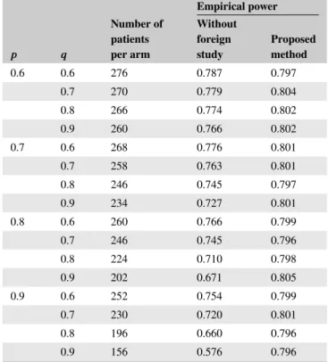
study. We used the same parameter values under the null and alternative hypotheses as before, and let 𝜏= 0. We set the number of patients per arm to 400 for the foreign study and varied𝑝and𝑞from 0.6 to 0.9. For each choice of(𝑝, 𝑞), we used the procedure described in Section 2.5 to determine the minimal sample size for achieving 80% power. We then con-ducted simulation with the resulting sample size to evaluate the power for the proposed testing procedure and compared it to the power without using the foreign-study evidence. Note that without using the foreign-study evidence, the required sample size to achieve the same power is at least 280 patients per arm.

The results are summarized in Table 1. The proposed method maintains the empirical power of 80%, and the effi-ciency gain, in terms of sample sizes, varies substantially with

(𝑝, 𝑞). The gain is small when𝑝or𝑞is less than 0.8. We can save the sample size by almost one half when both𝑝and𝑞are equal to 0.9.

4 DISCUSSION

In this article, we present a new framework for incorporat-ing the strength of evidence from a foreign study into the design and analysis of a bridging study. This framework relies on some Bayesian priors on the relationship between the hypotheses of the two studies and focuses on the adaptive type I error or power of the bridging study. The proposed methods account for randomness in the evidence of the foreign study so as to preserve the overall type I error. We develop a simple procedure to determine the optimal parameter that maximizes the conditional power for the bridging study.

(9)

T A B L E 1 Sample sizes for different choices of(𝑝, 𝑞)when𝜏= 0 Empirical power 𝒑 𝒒 Number of patients per arm Without foreign study Proposed method

0.6 0.6 276 0.787 0.797

0.7 270 0.779 0.804

0.8 266 0.774 0.802

0.9 260 0.766 0.802

0.7 0.6 268 0.776 0.801

0.7 258 0.763 0.801

0.8 246 0.745 0.797

0.9 234 0.727 0.801

0.8 0.6 260 0.766 0.799

0.7 246 0.745 0.796

0.8 224 0.710 0.798

0.9 202 0.671 0.805

0.9 0.6 252 0.754 0.799

0.7 230 0.720 0.801

0.8 196 0.660 0.796

0.9 156 0.576 0.796

decide on a clinically meaningful value of𝑝and𝑞, such that there is a modest gain in power.

The proposed methodology can be extended to incorporate multiple sources of evidence. When there are several foreign studies, the prior distributions for𝑝and𝑞are multivariate. The choice of the type I error on the prior distribution is also mul-tivariate and becomes more complicated because there may be some evidence favoring the null hypothesis and other evi-dence favoring the alternative hypothesis. The search for the optimal choice will be a grid search on a multidimension set. Alternatively, one may combine the multiple sources of evi-dence into a single measure (eg, some prespecified weighted combination), such that the methodology presented in this article can be applied directly.

Although this work is focused on incorporating foreign-study evidence into the design and analysis of a bridging study, the basic ideas are applicable to other contexts, where some prior study evidence is used to improve the design and analysis of a new study, for example, when historical data are incorporated into the design and analysis of a new clin-ical trial. By treating the prior study evidence as the “foreign study” evidence and the new study as the “bridging study,” the proposed methods can be applied directly.

Note that the proposed methodology allows the endpoints of the foreign and bridging studies to be different. This is a very useful feature because the indications for the drug prod-uct may be different between the new region and the original region or between the new study and the prior study within the same region. By contrast, Bayesian methods typically require

the same endpoint for the two studies so as to combine their likelihood functions.

ACKNOWLEDGMENTS

The authors wish to thank Dr. Richard Markus for reading the manuscript and providing helpful comments. They are grate-ful to an associate editor and two referees for their prompt reviews and constructive comments.

ORCID

Donglin Zeng https://orcid.org/0000-0003-0843-9280 D. Y. Lin https://orcid.org/0000-0002-0150-3115

R E F E R E N C E S

Chow, S.C., Chiang, C., Liu, J.-P. and Hsiao, C-F. (2012). Statistical methods for bridging studies.Journal of Biopharmaceutical Statis-tics, 22, 903–915.

Hsiao, C.-F., Hsu, Y.-Y., Tsou, H.-H. and Liu, J.-P. (2007). Use of prior information for Bayesian evaluation of bridging studies.Journal of Biopharmaceutical Statistics, 17, 109–121.

Huang, Q., Chen, G., Yuan, Z. and Lan, K.K.G. (2012). Design and sample size considerations for simultaneous global drug devel-opment program. Journal of Biopharmaceutical Statistics, 22, 1060–1073.

International Conference on Harmonization. (1998). Tripartite GUID-ANCE E5: Ethnic factors in the acceptability of foreign data.Federal Register, 83, 31790–31796.

Lan, K.K.G. and Pinheiro, J. (2012). Combined estimation of treatment effects under a discrete random effects model.Statistics and Bio-sciences, 4, 235–244.

Lan, K.K.G., Soo, Y., Siu, C. and Wang, M. (2005). The use of weighted Z-tests in medical research.Journal of Biopharmaceutical Statistics, 15, 625–639.

Liu, J.-P., Hsueh, H. and Chen, J. J. (2002). Sample size requirements for evaluation of bridging evidence.Biometrical Journal, 44, 969–981. Shih, W. J. (2001). Clinical trials for drug registration in Asian-Pacific

countries: proposal for a new paradigm from a statistical perspective. Controlled Clinical Trials, 22, 357–366.

Shao, J. and Chow, S.-C. (2002). Reproducibility probability in clinical trials.Statistics in Medicine, 21, 1727–1742.

SUPPORTING INFORMATION

Figure S1 referenced in Appendix A and Figures S2-S8 refer-enced in Section 3 are available with this article at the Biomet-rics website on Wiley Online Library. The simulation codes in this article are also available online with this article.

(10)

APPENDIX A: RELATIONSHIP BETWEEN

(𝒑, 𝒒)AND JOINT PRIOR DISTRIBUTION

OF (𝚫_𝟏,𝚫_𝟐)

Assume that the prior distribution for(Δ₁,Δ₂)is the bivari-ate normal distribution with mean (𝛿₁, 𝛿₂) and covariance matrix

Σ = (

𝜎2

1 𝜌𝜎1𝜎2 𝜌𝜎₁𝜎₂ 𝜎2

2 )

.

Then

𝑝=Pr(𝐻₁₀|𝐻₂₀) =Pr{Δ₁∉ (𝐿₁, 𝑈₁)|Δ₂∉ (𝐿₂, 𝑈₂)}

= ∫(−∞,𝐿1]∪[𝑈1,∞)∫(−∞,𝐿2]∪[𝑈2,∞)(2𝜋)

−1_|_Σ_|−1∕2_exp{−(_𝑥₋_𝛿

1, 𝑦−𝛿2)Σ−1(𝑥−𝛿1, 𝑦−𝛿2)T}𝑑𝑦 𝑑𝑥

Φ((𝐿₂−𝛿₂)∕𝜎₂) + Φ(−(𝑈₂−𝛿₂)∕𝜎₂) ,

and

𝑞=Pr(𝐻₁_𝑎|𝐻₂_𝑎) =Pr{Δ₁∈ (𝐿₁, 𝑈₁)|Δ₂∈ (𝐿₂, 𝑈₂)}

= ∫

𝑈1

𝐿1 ∫

𝑈2

𝐿2 (2𝜋)

−1_|_Σ_|−1∕2_exp{−(_𝑥₋_𝛿

1, 𝑦−𝛿2)Σ−1(𝑥−𝛿1, 𝑦−𝛿2)𝑇}𝑑𝑦 𝑑𝑥

−Φ((𝐿₂−𝛿₂)∕𝜎₂) + Φ((𝑈₂−𝛿₂)∕𝜎₂) .

We provide an example to illustrate the above relation-ship. Let 𝐿₁=𝐿₂= −0.75 and 𝑈₁=𝑈₂= 0.75. Also, let 𝛿₁=𝛿₂= 0 and 𝜎₁=𝜎₂= 1. Figure S1 in the Supporting Information shows how𝑝and𝑞vary with the correlation coef-ficient𝜌. The higher the correlation in the joint prior distribu-tion is, the larger the values of𝑝and𝑞are.

APPENDIX B: PROOFS OF THEOREMS Proof of Theorem1. Note that

Pr((𝜔, 𝛾)|𝐻₂₀)

=Pr(the bridging study is conducted andCI₂(̂𝛼₂)

⊂(𝐿₂, 𝑈₂)|𝐻₂₀)

=Pr(CI₁(𝜔)⊂(𝐿₁, 𝑈₁),CI₂(𝛼𝛾)⊂(𝐿₂, 𝑈₂)|𝐻₂₀)

+ (1 −𝜏)Pr(CI₁(𝜔)⊊(𝐿₁, 𝑈₁),CI₂(𝛼∕𝛾)

⊂(𝐿₂, 𝑈₂)|𝐻₂₀).

Under Assumption 1, the last expression is equal to

Pr(𝐻₁₀|𝐻₂₀)Pr(CI₁(𝜔)⊂(𝐿₁, 𝑈₁)|𝐻₁₀)

×Pr(CI₂(𝛼𝛾)⊂(𝐿₂, 𝑈₂)|𝐻₂₀)

+Pr(𝐻₁_𝑎|𝐻₂₀)Pr(CI₁(𝜔)⊂(𝐿₁, 𝑈₁)|𝐻₁_𝑎)

×Pr(CI₂(𝛼𝛾)⊂(𝐿₂, 𝑈₂)|𝐻₂₀)

+Pr(𝐻₁₀|𝐻₂₀)(1 −𝜏)Pr(CI₁(𝜔)⊊(𝐿₁, 𝑈₁)|𝐻₁₀)

×Pr(CI₂(𝛼∕𝛾)⊂(𝐿₂, 𝑈₂)|𝐻₂₀)

+Pr(𝐻₁_𝑎|𝐻₂₀)(1 −𝜏)Pr(CI₁(𝜔)⊊(𝐿₁, 𝑈₁)|𝐻₁_𝑎)

×Pr(CI₂(𝛼∕𝛾)⊂(𝐿₂, 𝑈₂)|𝐻₂₀),

which can be bounded by

𝑝𝜔𝛼𝛾+ (1 −𝑝)𝛼𝛾Pr(CI₁(𝜔)⊂(𝐿₁, 𝑈₁)|𝐻₁_𝑎) +𝑝(1 −𝜏)(1 −𝜔)𝛼∕𝛾

+ (1 −𝑝)(1 −𝜏)𝛼∕𝛾Pr(CI₁(𝜔)⊊(𝐿₁, 𝑈₁)|𝐻₁_𝑎).

Thus,

Pr((𝜔, 𝛾)|𝐻₂₀)

≤𝑝𝜔𝛼𝛾+𝑝(1 −𝜏)(1 −𝜔)𝛼∕𝛾+ (1 −𝑝)𝛼max(𝛾,(1 −𝜏)∕𝛾) ≤𝑝𝜔𝛼𝛾+𝑝(1 −𝜏)(1 −𝜔)𝛼∕𝛾+ (1 −𝑝)𝛼𝛾

≤𝛼[{1 −𝑝+𝑝𝜔}𝛾+𝑝(1 −𝜔)(1 −𝜏)∕𝛾]

≤𝛼[{1 −𝑝+𝑝𝜔}𝛾+𝑝(1 −𝜔)∕𝛾]. (A1)

The conclusion of Theorem 1 follows upon verifying that𝛾 given in Theorem 1 ensures that (A1) is bounded by𝛼. □

Proof of Theorem2. Clearly,

Pr((𝜔, 𝛾)|𝐻₂_𝑎)

(11)

=Pr(CI₁(𝜔)⊂(𝐿₁, 𝑈₁),CI₂(𝛼𝛾)⊂(𝐿₂, 𝑈₂)|𝐻₂_𝑎)

+ (1 −𝜏)Pr(CI₁(𝜔)⊊(𝐿₁, 𝑈₁),CI₂(𝛼∕𝛾) ⊂(𝐿₂, 𝑈₂)|𝐻₂_𝑎).

Under Assumption 2,

Pr(the bridging study is conducted andCI₂(̂𝛼₂)

⊂(𝐿₂, 𝑈₂)|𝐻₂_𝑎)

=Pr(𝐻₁_𝑎|𝐻₂_𝑎)Pr(CI₁(𝜔)⊂(𝐿₁, 𝑈₁)|𝐻₁_𝑎)

×Pr(CI₂(𝛼𝛾)⊂(𝐿₂, 𝑈₂)|𝐻₂_𝑎)

+Pr(𝐻₁_𝑎|𝐻₂_𝑎)(1 −𝜏)Pr(CI₁(𝜔)⊊(𝐿₁, 𝑈₁)|𝐻₁_𝑎)

×Pr(CI₂(𝛼∕𝛾)⊂(𝐿₂, 𝑈₂)|𝐻₂_𝑎)

+Pr(𝐻₁₀|𝐻₂_𝑎)Pr(CI₁(𝜔)⊂(𝐿₁, 𝑈₁)|𝐻₁₀)

×Pr(CI₂(𝛼𝛾)⊂(𝐿₂, 𝑈₂)|𝐻₂_𝑎)

+Pr(𝐻₁₀|𝐻₂_𝑎)(1 −𝜏)Pr(CI₁(𝜔)⊊(𝐿₁, 𝑈₁)|𝐻₁₀)

×Pr(CI₂(𝛼∕𝛾)⊂(𝐿₂, 𝑈₂)|𝐻₂_𝑎).

It follows from the definition of𝑄_𝑘(𝛼₀)that Pr((𝜔, 𝛾)|𝐻₂_𝑎)

=𝑞{𝑄₂(𝛼𝛾)Pr(CI₁(𝜔)⊂(𝐿₁, 𝑈₁)|𝐻₁_𝑎)

+ (1 −𝜏)𝑄₂(𝛼∕𝛾)[1 −Pr(CI₁(𝜔)⊂(𝐿₁, 𝑈₁)|𝐻₁_𝑎)]}

+ (1 −𝑞)𝜔𝑄₂(𝛼𝛾) + (1 −𝑞)(1 −𝜏)(1 −𝜔)𝑄₂(𝛼∕𝛾)

=𝑞{𝑄₂(𝛼𝛾)𝑄₁(𝜔) + (1 −𝜏)𝑄₂(𝛼∕𝛾)[1 −𝑄₁(𝜔)]}

+ (1 −𝑞)𝜔𝑄₂(𝛼𝛾) + (1 −𝑞)(1 −𝜏)(1 −𝜔)𝑄₂(𝛼∕𝛾).

If 𝜔= 1, then 𝛾 in Theorem 1 is equal to 1, such that we do not use the evidence from the foreign study. It follows that𝑄̃₂(1) =𝑄₂(𝛼). Therefore, the second part of Theorem 2