LOCOMOTION AND BALANCE CONTROL OF HUMANOID ROBOTS WITH DYNAMIC AND KINEMATIC CONSTRAINTS
Yu Zheng
A dissertation submitted to the faculty of the University of North Carolina at Chapel Hill in partial fulfillment of the requirements for the degree of Doctor of Philosophy in the
Department of Computer Science.
Chapel Hill 2014
©2014 Yu Zheng
ABSTRACT
Yu Zheng: Locomotion and Balance Control of Humanoid Robots with Dynamic and Kinematic Constraints
(Under the direction of Katsu Yamane and Ming C. Lin)
Building a robot capable of servicing and assisting people is one of the ultimate goals in humanoid robotics. To realize this goal, a humanoid robot first needs to be able to perform some fundamental locomotion tasks, such as balancing and walking. However, simply performing such basic tasks in static, open environments is insufficient for a robot to be useful. A humanoid robot should also possess the ability to make use of the object in the environment to generate dynamic motions and improve its mobility. Also, since humanoid robots are expected to work and live closely with humans, having human-like motions is important for them to be human-friendly.
that computes the desired acceleration to track the given reference motion and an optimizer that computes the optimal joint torques and contact forces to realize the desired acceleration, considering the full-body dynamics of the robot and strict constraints on contact forces. By taking advantage of the property that the joint torques do not contribute to the six degrees of freedom of the floating base, I decouple the computation of joint torques and contact forces such that the optimization problem with strict contact force constraints can be solved in real time. In full-body simulation, a humanoid robot is able to imitate various human motions by using this method.
ACKNOWLEDGEMENTS
The past four and a half years I spent at the Department of Computer Science of the University of North Carolina (UNC) at Chapel Hill and Disney Research Pittsburgh (DRP) on the research that eventually turned into this dissertation have been truly memorable. I would like to thank people who made my journey so special and extraordinary. First of all, I would like to thank my advisor at UNC, Prof. Ming Lin, and my advisor at DRP, Dr. Katsu Yamane, for their elaborate guidance and altruistic support, as well as the freedom I was provided throughout my work. I would also like to thank my co-advisor at UNC, Prof. Dinesh Manocha, for his collaboration and invaluable suggestions. I would also like to thank the other members of my committee, Prof. Ron Alterovitz and Prof. Jack Snoeyink, for their insightful feedback and discussions on my research work and this dissertation.
I would like to thank many other talented collaborators, colleagues, and friends who have helped me with my work and study, including Matt Glisson, Michael Mistry, Akihiko Murai, Hengchin Yeh, Feng Zheng, and Tian Cao. I would also like to thank many anonymous reviewers who have helped me improve the quality of my work.
I want to express my special thanks to Disney Research Pittsburgh for having me there and supporting my work and also Carnegie Mellon University, especially Prof. Jessica Hodgins and Prof. Chris Atkeson, for letting me use the CMU Sarcos Humanoid Robot for my experiments.
TABLE OF CONTENTS
LIST OF TABLES . . . xi
LIST OF FIGURES . . . xii
LIST OF ABBREVIATIONS . . . xvi
1 INTRODUCTION . . . 1
1.1 Locomotion Generation Overview . . . 2
1.1.1 Environmental Property . . . 3
1.1.2 Robot Model . . . 3
1.1.3 Sensor Information . . . 3
1.1.4 Framework for Motion Generation and Verification . . . 4
1.2 Locomotion of Humanoid Robots . . . 5
1.2.1 Robot Balance Control . . . 5
1.2.2 Biped Locomotion Generation . . . 6
1.2.3 Motion Tracking Control . . . 7
1.3 Thesis Statement . . . 8
1.4 Main Results . . . 9
1.4.1 Balance Control in a Dynamic Environment . . . 9
1.4.2 Manipulating a Dynamic Object by Active Walking . . . 9
1.4.3 Motion Tracking under Strict Contact Constraints . . . 10
2 BALANCE CONTROL ON A DYNAMIC OBJECT . . . 11
2.1 Introduction . . . 11
2.2 Previous Work . . . 12
2.3 Problem Overview . . . 13
2.3.1 Problem Statement . . . 13
2.3.2 Control Framework . . . 14
2.4 Balance Controller . . . 15
2.4.1 Flat-Foot Sagittal-Plane Simplified Model . . . 16
2.4.2 Geta-Foot Sagittal-Plane Simplified Model . . . 18
2.4.3 Frontal-Plane Simplified Model . . . 18
2.4.4 Balance Controller for the Sagittal-Plane Motion . . . 19
2.4.5 Balance Controller for the Frontal-Plane Motion . . . 21
2.4.6 Computation of the Desired COP . . . 22
2.5 System Measurement . . . 24
2.5.1 COM Measurement . . . 25
2.5.2 COP Measurement . . . 25
2.5.3 Configuration Measurement of the Simplified Models . . . 27
2.6 Full-Body Mapping and Simulation . . . 28
2.6.1 Torque Mapping . . . 28
2.6.2 Simulation. . . 31
2.7 Experiments on the Sarcos Humanoid Robot . . . 32
2.8 Conclusions and Future Work . . . 34
3 MANIPULATING A DYNAMIC OBJECT BY ACTIVE WALKING . . . 36
3.1 Introduction . . . 36
3.1.1 Main Results . . . 36
3.1.2 Organization . . . 37
3.2 Previous Work . . . 37
3.2.2 Limit Cycle Walking of Passive Walkers . . . 38
3.3 Static Walking Gait Generation . . . 39
3.3.1 Frontal Motion Planner . . . 39
3.3.2 Sagittal Motion Planner . . . 41
3.3.3 Simulation Results . . . 44
3.4 Cyclic Walking Gait Generation . . . 45
3.4.1 Equation of Motion . . . 46
3.4.2 Collision Model . . . 48
3.4.3 Computing a Cyclic Walking Gait . . . 52
3.4.3.1 Cost Function of the Optimization . . . 52
3.4.3.2 Constraints of the Optimization . . . 55
3.4.4 Maintaining a Cyclic Walking Gait . . . 56
3.4.4.1 Inverse Kinematics . . . 56
3.4.4.2 Initial State for the Next Step . . . 57
3.4.5 Simulation Results . . . 59
3.4.5.1 Setup for Optimization . . . 59
3.4.5.2 Optimal Cyclic Gait . . . 59
3.4.5.3 Simulation Under Disturbance . . . 61
3.5 Conclusions and Future Work . . . 62
4 MOTION TRACKING CONSIDERING STRICT CONTACT CONSTRAINTS . . 66
4.1 Introduction . . . 66
4.1.1 Main Results . . . 67
4.1.2 Organization . . . 68
4.2 Previous Work . . . 68
4.3 Full-Body Dynamics of a Humanoid Robot . . . 69
4.4.1 Proportional-Derivative (PD) Controller . . . 73
4.4.2 Joint Torque Optimization Module . . . 74
4.4.2.1 Step 1—Computing contact forces . . . 75
4.4.2.2 Step 2—Computing joint torques . . . 76
4.5 Computation of Contact Forces . . . 78
4.5.1 Basic Formulations . . . 79
4.5.2 Computing Feasible Contact Forces . . . 83
4.5.3 Computing Minimum Contact Forces . . . 86
4.6 Simulation . . . 90
4.6.1 Simulation Setup . . . 90
4.6.2 Tracking Human Motion Without Contact State Change . . . 90
4.6.3 Tracking Human Motion With Contact State Change . . . 92
4.6.4 Tracking Extreme Reference Motion . . . 93
4.7 Conclusions and Future Work . . . 95
5 CONCLUSION. . . 98
LIST OF TABLES
LIST OF FIGURES
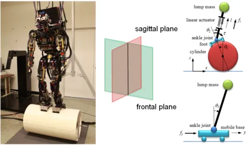
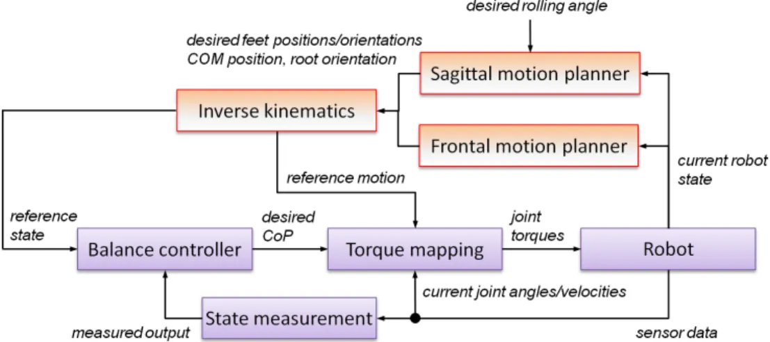
2.1 Sarcos humanoid robot standing on a free-rolling cylinder. The 3-D motion of the robot with the cylinder is decomposed into two 2-D motions in the sagittal and frontal planes, for which different
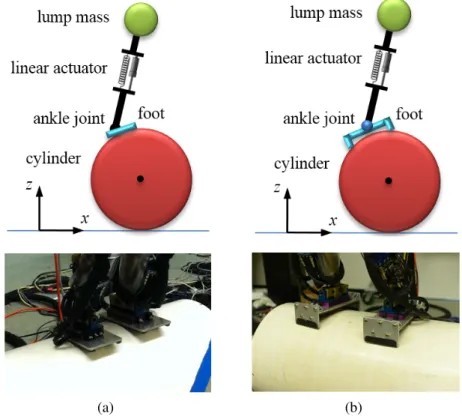
simplified models are used in designing balance controllers. . . 14 2.2 Simplified dynamics model for a biped robot with (a) flat feet or
(b) geta feet on a rolling cylinder in the sagittal plane. . . 15 2.3 Control framework. . . 16 2.4 Simplified dynamics model of a biped robot with flat feet on a
rolling cylinder in the sagittal plane. (a)θ0 is the rolling angle of the cylinder, which also indicates the relative position of the ankle joint to the top of the cylinder if the ankle joint is initially above the top. (b)θ1is the rolling angle of the foot relative to the cylinder. (c)θ2 is the angle of the ankle joint, indicating the center of mass
(COM) position relative to the ankle. (d)lis the change of the distance. . . 16 2.5 Measurement of the actual COP and the state of (a) the flat-feet
model or (b) the geta-feet model. . . 25 2.6 Simulation of a biped robot with (a) flat feet or (b) geta feet on a
rolling cylinder. The blue arrow represents the external disturbance
applied to the robot. . . 32 2.7 Experimental setup on the Sarcos humanoid robot. . . 33 2.8 Conversion of the desired COP to the foot rotation. (a) The
de-sired COP moving forward. (b) Increasing the ankle torque in the
direction as shown. (c) Extending the feet. . . 34
3.1 Framework for walking motion generation on a rolling cylinder. . . 40 3.2 Framework for sagittal walking motion generation on a rolling cylinder. . . 41 3.3 Illustration of the motion of the swing foot in a step. The swing foot
(in the blue color) (a) rotates together with the supporting foot (not shown) and rolls the cylinder for angleα, (b) lifts up, (c) moves backwards, and then (d) touches down. Once touching down, the swing foot becomes the supporting foot (in the green color) for the next step and (e) rotates and rolls the cylinder for another angleα. (a) and (e) happen at the same time in one step on the swing foot
3.4 Snapshots of biped walking on a rolling cylinder. (a) Initial pose. (b) Moving the weight to the left foot and lifting up the right foot. (c) Touching down the right foot at a position behind the left foot. (d) Rotating the cylinder forward while moving the weight to the right. (e)-(g) Repeating this procedure with the right foot as the
supporting foot and the left foot as the swing foot. . . 45 3.5 Graphs of (a,b) the reference and actual COM trajectories and (c,d)
the desired, optimized, and actual COP trajectories. . . 46 3.6 Collision model. The motion of the cylinder is described using
vari-ablesxo, yo, θ0, while that of each leg is described using variables x, y, α, θ2, l. The subscriptscandsrepresent the colliding (swing)
leg and the supporting leg, respectively. . . 47 3.7 Distribution of optimal initial states in the state space. Blue and
red dots represent the optimal initial sates with smaller and larger
values of the cost function defined by (3.32). . . 60 3.8 Distribution of optimal initial states with smaller (marked in green)
and larger (marked in red) energy consumption for one step. . . 60 3.9 Optimal initial states colored according to the change in the cost
function while shifting optimal initial states in the normal direction.
The yellow (red) color means that the change is relatively smaller (bigger). . . 61 3.10 One hundred walking cycles starting with an optimal initial state.
Each curve from a dot to a square represents a step. The red color denotes the first step starting with the optimal initial state, while
the blue color denotes the last step. . . 62 3.11 Walking cycles under disturbances in the model and the ankle
torque. The red color denotes the first step starting with the optimal initial state, while the green and blue colors denote the last two
steps, which are slightly different due to the random disturbance. . . 63 3.12 Walking cycles with desired average velocity equal to0.4 rad/s. . . 64 3.13 Snapshots of one cyclic step with average velocity equal to (a)
0.2 rad/sand (b)0.4 rad/sunder different disturbances. . . 65
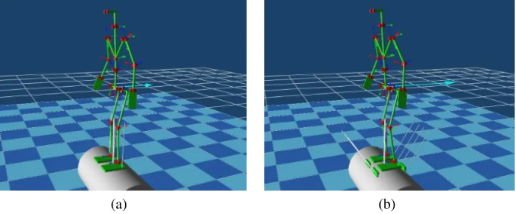
4.1 Example of human motion tracking. (a) The original human motion.
(b) The simulated robot motion. . . 67 4.2 Illustration of the relationship between the contact wrench applied
4.3 Overview of the motion tracking controller consisting of two main steps in the dashed box: 1) computation of the contact wrenches to realize the desired floating-base motion, and 2) computation of the joint torques to realize the desired full-body motion. The symbols
are defined in the text. . . 73 4.4 Illustration of the algorithm in 3-D space to compute the minimum
distance betweenwandV = CO(W). By iteration it generates a sequence of simplicial conesCO(Vk)in the convex coneCO(W) such that the pointvk inCO(Vk)having the minimum Euclidean distance to the pointwconverges to the closest point inCO(W)to
w. Then, the distance between them gives the Euclidean separation
distance betweenCO(W)andw. . . 83 4.5 Illustration of two iteration strategies to compute the minimum
contact forces. (a) A subsetVk+1ofW −zkis computed at every iteration byAlgorithm 1such thatwˆis a positive combination of Vk+1. Then,zk+1, a convex combination ofZk+1 =Vk+1+zk that is proportional towˆ, is closer tozthanzk. Hence,zkapproaches
zas the iteration proceeds. (b)CH(Z)k(red triangle) is a facet in W such that its interior contains a pointzkproportional towˆ and
nkis the normal of the facet such thatnTkwˆ >0. Using a subset of the vertices ofCH(Z)kandsW(nk), I can find a new facet (green triangle) that contains a new pointzk+1in the directionwˆ strictly closer tozthanbk. This iteration can proceed untilzkconverges
toz, provided thatzk+1 always lies in the interior of the new facet. . . 87 4.6 Example of (a) original and (b) simulated motion of “I’m a little
teapot” performed by subject 1. . . 91 4.7 Example of (a) original and (b) simulated motion of “I’m a little
teapot” performed by subject 2. . . 92 4.8 Optimized (red) and actual (blue) contact forces and moments on
the left foot. . . 93 4.9 Simulated side stepping motion. . . 94 4.10 Simulated forward stepping motion. . . 95 4.11 Optimized (red) and actual (blue) contact forces in x- and z-directions
and moments in y-direction on the left (upper) and right (below)
4.12 Example of preventing falling in tracking extreme motions. (a) Unbalanced reference pose for tracking (transparent) and static equilibrium pose for falling prevention (opaque). (b) Final pose of the robot, which is close to but does not reach the tracking reference pose. (c) The contact forces at the local COP on each foot (white lines) and the total contact force at the global COP (red line), which
LIST OF ABBREVIATIONS
COM Center of Mass COP Center of Pressure DOF Degree of Freedom
CHAPTER 1: INTRODUCTION
Robots have the potential to significantly change human life in the 21st century. Robotics research is essential in bringing robots to benefit our daily lives. Of particular interest is research into humanoid robotics, whose ultimate goal is to build a robot that not only looks but also behaves like a human, and may even become more capable than a human. To realize this goal, a humanoid robot needs first to be able to conduct the tasks fundamental to legged robots, such as balancing and walking. However, simply performing such basic tasks in static, open environments is far from enough for a robot to be useful. A humanoid robot should also possess the ability to make use of external tools or objects, such as a bicycle and a skateboard, to generate dynamic motions and improve its mobility. Then, the ability to manipulate or maneuver external tools or objects must be considered together with the locomotion of the robot itself. Also, humanoid robots are expected to work and live closely with humans, so having human-like motions is important for them to be human-friendly and finally merge into the human society. In some applications, such as performing a drama and conducting an orchestra on the stage, a humanoid robot must be capable of providing stylized human-like motions. In all such scenarios, a humanoid robot needs to not only perform a single basic locomotion task, such as balancing or walking, but also achieve other goals, such as manipulating an object or imitating human motions.
locomotion task is challenging even for normal humans. There are many problems that need to be solved to make it happen on a humanoid robot. For example, one essential problem is how to design controllers to control not only the motion of the robot but also the cylinder’s motion. A further problem is what walking gait the robot should and can perform on top of the cylinder in order to roll the cylinder. In tackling these problems, many factors need to be considered, such as the dynamics of the robot and the cylinder, the impact when the swing foot leaves or touches the cylinder, various physical and dimensional constraints, disturbances and errors that may cause the robot to deviate from a planned gait, and so on.
Second, I present a method for humanoid robots to track given reference motions, such as captured human motions or motions defined by key frame animation, such that they can have human-like or stylized motions. The motion of a floating-base humanoid robot depends not only on the joint torques but also the reaction contact forces from the environment, which are dependent on the applied joint torques and subject to the nonlinear friction constraints. Direct proportional-derivative (PD) tracking usually does not work in this case because the desired joint accelerations from traditional PD control law are not necessarily achievable due to the limitation in friction. Also, the contact links of the robot in a reference motion usually do not comply with the current environment and a kinematic constraint needs to be imposed on each of them to correct their motions. Therefore, how to take into account these constraints in motion tracking, while keeping the computation fast enough for real-time control, is a challenging problem.
1.1 Locomotion Generation Overview
common information and components are required by almost all the methods. In this section, I provide a high-level introduction.
1.1.1 Environmental Property
Locomotion generation must take into account the environmental property for a gener-ated motion to be consistent with and physically achievable in the environment. First, the geometric information of the environment needs to be considered. For example, to generate a walking behavior, we need to know whether it happens on a horizontal ground, slopes, stairs, or even rough terrains, so that specific motion strategies can be used. Second, we need to know some physical parameters, such as the friction coefficient. If the robot is required to interact with some dynamic objects in the environment, then the kinematic and dynamic properties of the objects should be known as well.
1.1.2 Robot Model
In order to generate a motion that a robot can carry out, the model of the robot, including its kinematic and dynamic parameters, must be known. The kinematic parameters include the structure (the number and types of joints and their arrangement) and the dimension (the size of each link) of the robot, which are needed in both kinematics and dynamics calculations. The dynamic parameters include the mass and inertia and the position of the center of mass of each link, which are used together with the kinematic parameters in the forward/inverse dynamics calculation.
1.1.3 Sensor Information
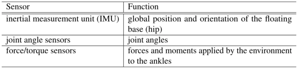
measure its orientation and acceleration. Second, force-torque sensors are common sensors installed on robot’s feet to measure the contact forces applied to the feet by the environment. Using the force-torque sensor data, we can also estimate the position of the center of pressure (COP), which plays an important role in the balance control of a humanoid robot. Third, joint angle sensors are usually embedded in every joint to record the joint angle and velocity. Those data are required by many components in the locomotion generation and control, such as the design of controllers and the calculation of the full-body dynamics of the robot. Depending on the requirement of a locomotion task, other sensors or sensing techniques may be used as well, such as vision sensors and ultrasonic sensors. In my work, I only use the aforementioned three conventional sensors.
1.1.4 Framework for Motion Generation and Verification
angles for position-controlled robots or joint torques for torque-controlled robots, and the ways to perform this conversion are different.
The robot in simulation or hardware accepts the control command and should produce the planned motion if the designed controllers work properly. However, it is inevitable that the model used to compute the control command has some difference from the real robot. Due to the modeling error, the robot usually does not generate the exactly same motion as the planed one and a difference always exists between them. Then, the controllers are expected to capture this difference and consider it in the computation of the control command, typically through feedback, so as to correct the generated motion.
In this dissertation, I focus on the control unit, including balance control, walking gait generation, and motion tracking control.
1.2 Locomotion of Humanoid Robots
Nowadays, many robots are capable of basic locomotion tasks, such as walking and running (Takanishi et al., 1988; Kajita et al., 2005), and many methods for locomotion generation and control of humanoid robots have been proposed. The following subsec-tions discuss well-known approaches that are closely related to the work presented in this dissertation.
1.2.1 Robot Balance Control
model to produce the desired positions of the ZMP and the center of mass (COM) for the robot to maintain balance. The control command for the robot to generate the full-body motion and realize those positions, namely joint angles for position-control robots or joint torques for torque-controlled robots, is computed through inverse kinematics or inverse dynamics (Kajita et al., 2003; Yamane and Hodgins, 2009). One major issue with this method is that the ZMP-based feasibility criterion is only applicable to horizontal terrains. Ott et al. (2011) used a more general criterion based on feasible contact forces and developed a balance controller that can be applied to any terrains.
The above work assumes that the robot is in a stationary environment. So far, the study of robot balance control in non-stationary environments is still limited. Kuroki et al. (2003; 2004) proposed a motion control system to maintain balance of a small biped robot on a moving platform or under external forces. For the same purpose, Hyon (2009) presented a contact force control framework for the balance control of a human-size robot on rough terrains under external forces, while Anderson and Hodgins (2010) developed methods for adapting models of humanoid robots performing dynamic tasks. However, these control techniques only allow robot to passively adapt to the environmental change and cannot be used in the balance control by manipulating a dynamic object as I do in this dissertation.
1.2.2 Biped Locomotion Generation
(Sug-ihara et al., 2002; Kajita et al., 2003). In an environment with known obstacles, several algorithms have been proposed to compute footsteps and a collision-free path for a biped robot (Kuffner et al., 2001; Chestnutt et al., 2005; Ayaz et al., 2009), such that the walking pattern can be generated later in this way. Some work tried to mimic human walking motion by adding single toe support phase and characterized swing leg motions (Miura et al., 2011). To avoid using the ZMP feasibility criterion and generate biped walking on uneven terrain, Hirukawa et al. (2006) proposed a walking pattern generator using a general criterion based on feasible contact forces.
Humanoid locomotion can also be generated in a reverse way. One may first generate a reference COM or upper-body motion for the robot. Then, the required COP trajectory is computed from the reference reference motion based on a simplified model, and appropriate footsteps that cover the computed COP trajectory are also determined. Finally, full-body trajectories in terms of joint angles of the robot can be calculated likewise through inverse kinematics. Unfortunately, there is not much work on this kind of methods (Sugihara, 2008).
The above walking generation methods consider the robot to walk on the ground that does not move. Hence, they cannot be used in my case where a robot is required to walk on a dynamic object and manipulate the object by bipedal walking.
1.2.3 Motion Tracking Control
trajectory that ensures the dynamic consistency. Nakaoka et al. (2003) proposed a method to convert human dancing motions to physically feasible motions for humanoid robots by manually segmenting a motion into motion primitives and designing a controller for each of them. However, these approaches are aimed at offline planning.
Some methods can realize online tracking of upper-body motions in the double-support phase while using the lower body for balancing (Zordan and Hodgins, 2002; Ott et al., 2008). Yamane and Hodgins (2009; 2010) presented controllers for humanoid robots to simultaneously track motion capture data and maintain balance. However, most of the previous work omitted the friction constraint on contact forces by assuming that the friction coefficient is big enough or considered it as a penalty term in the computation to simplify the problem. As a consequence, the generated motion may cause the violation of the friction constraint and not be achievable in practice.
Using human motion data to generate motion for humanoid characters has also been studied in computer graphics (Tak et al., 2000; Safonova et al., 2004; Sok et al., 2007; da Silva et al., 2008; Muico et al., 2009). Nevertheless, those approaches usually employ an extensive optimization process and cannot be applied to realtime control of humanoid robots.
Developing efficient methods for realtime motion tracking for humanoid robots consid-ering strict friction and other constraints still remains to be a difficult problem.
1.3 Thesis Statement
Considering dynamic and kinematic constraints in the environment in the controller
design enables humanoid robots to enhance locomotion tasks by manipulating a dynamic
1.4 Main Results
In support of my thesis statement, I present several major results on generating dynamic, human-like motions on humanoid robots. First, I demonstrate how to design a balance controller such that a humanoid robot maintains balance on an object that will move because of the interaction with the robot. Second, I discuss how to actively manipulate such a dynamic object and control its motion by generating walking behaviors on top of it to improve the mobility of the robot itself. Finally, I provide a method for enabling humanoid robots to produce stylized motions using motion capture data.
1.4.1 Balance Control in a Dynamic Environment
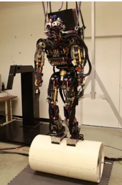
One important result included in this dissertation is a balance control technique for a humanoid robot having interaction with dynamic objects in the environment. Taking a cylinder that rolls freely on the ground as an example, I present a balance controller such that a humanoid robot can balance on the cylinder under disturbances. In order for the robot to actively maneuver cylinder’s motion rather than passively adapt to it, I take into account the dynamics of the cylinder together with that of the robot in the balance controller design. This technique can potentially be applied to the balance control of humanoid robots in other similar scenarios, such as riding a unicycle or pushing a wheelbarrow, as long as the dynamics of the object or the tool that the robot operates can be modelled. Using the proposed balance controller, I enable a real robot, the Sarcos humanoid robot, to balance on a free-rolling cylinder. These results will be discussed in Chapter 2.
1.4.2 Manipulating a Dynamic Object by Active Walking
pattern and roll the cylinder at a desired speed. A collision model between the swing leg and the cylinder is derived to compute the velocity change of the robot and the cylinder when the swing leg touches down. I also present a method for the robot to maintain a planned gait under disturbances. These results will be addressed in Chapter 3.
1.4.3 Motion Tracking under Strict Contact Constraints
Additionally, in this dissertation I present a motion tracking control method for hu-manoid robots to reproduce given reference motions, such as motions defined by human motion capture data or key frame animation. The method considers the exact full-body dynamics of the robot and the strict friction constraint on contact forces. By taking advan-tage of the property that the joint torques do not contribute to the six DOFs of the floating base of the robot, I separate the computation of contact forces from joint torques. As a result, computing the contact force that satisfies the friction constraint can be reduced to a simple quadratic program with second-order cone constraints, for which I present several efficient algorithms. Once the contact forces are determined, the optimal joint torques can be computed in a closed form. While the solution satisfies strict friction constraints, this method is fast enough for realtime motion tracking and can be applied to motions on uneven terrains or involving contacts at hands or links other than robot’s feet. These results will be discussed in Chapter 4.
CHAPTER 2: BALANCE CONTROL ON A DYNAMIC OBJECT
2.1 Introduction
Most of the previous work on robot locomotion assumes a stationary environment and considers only the motion of the robot itself. For a robot to be truly useful for humans, however, it should also be able to manipulate objects and make changes in the environment while performing a basic locomotion task. Such capability is often required in our daily activities, such as pushing a cart while wandering in a supermarket. In this and the next chapters I discuss how I realize a generic biped humanoid robot that actively manipulates an object in the environment and performs a dynamic motion. In this particular piece of work, I choose walking on a free-rolling cylinder as an example of such behaviors, which is difficult even for normal humans. Considering cylinder’s movement is mandatory because the interaction with the environment is limited to the contact between the cylinder and floor. This chapter introduces the development of a balance controller that enables a humanoid robot to stand and maintain balance on the cylinder. The balance controller provides the basis for generating biped walking behaviors of the robot on the cylinder, which will be discussed in the next chapter.
2.1.1 Main Results
In order for the robot to actively maneuver cylinder’s motion rather than passively adapt to it, I take into account the dynamics of the cylinder together with robot’s own dynamics in the development of the balance controller and the tracking controller. Both simulation and hardware experimental results are provided at the end of this chapter to show the effectiveness of this balance control method.
2.1.2 Organization
This chapter is organized as follows. Section 2.2 briefly reviews the related work. Section 2.3 gives an overview of my work on balance control. Section 2.4 describes the simplified model and the details of the balance controller. Section 2.5 discusses available sensors and system measurement based on sensor data. Section 2.6 details the joint torque computation and full-body simulation. Section 2.7 reports the experiment on a real humanoid robot. In Section 2.8, I discuss the limitation and the possible extension of this work.
2.2 Previous Work
So far, the study of robot motion control in non-stationary environments is still limited. Kuroki et al. (2003; 2004) proposed a motion control system to maintain balance of a small biped robot on a moving platform or under external forces. For the same purpose, Hyon (2009) presented a contact force control framework for the balance control of a human-size robot on rough terrains under external forces, while Anderson and Hodgins (2010) developed methods for adapting models of humanoid robots performing dynamic tasks. In these cases, however, the robot’s feet keep stationary contact with the platform or ground and no stepping motion is involved.
Besides humanoid robots, some other robots may work in a non-stationary environment, such as a singe spherical wheeled mobile robot (Nagarajan et al., 2009, 2013) and multi-wheeled robots balancing on and driving a ball (Endo and Nakamura, 2005; Lauwers et al., 2006; Kumagai and Ochiai, 2009). In that case, the wheels always make three or four symmetric contacts with the ball, which greatly benefits the balance control of the robot. In my case, however, the feet of a biped robot can only make one or two contacts with a cylinder, which are usually asymmetrical about the top of the cylinder. Furthermore, because of the limited foot size and support region, the ideal COP, which is continuously changing on a rolling cylinder, may go beyond the support region. Hence, I have to not only design controllers to maintain system’s balance but also combine them with a stepping motion generator to provide the robot with timely support on the rolling cylinder during walking, which will be discussed in the next chapter.
2.3 Problem Overview
2.3.1 Problem Statement
Figure 2.1. Sarcos humanoid robot standing on a free-rolling cylinder. The 3-D motion of the robot with the cylinder is decomposed into two 2-D motions in the sagittal and frontal planes, for which different simplified models are used in designing balance controllers.
contact with the cylinder, so the foot can rotate about the edge relative to the cylinder, which gives the robot more degrees of freedom but makes the balance control more difficult. By contrast, a geta foot, which is built by attaching an extra plate to both toe and heel sides of a normal flat foot, can contact the cylinder by two edges. Then, the geta foot cannot move relative to the cylinder while maintaining the full contact, assuming that it does not slip either. The two contact edges form a much bigger rectangular support region for the robot, which significantly facilitates the balance control.
2.3.2 Control Framework
(a) (b)
Figure 2.2. Simplified dynamics model for a biped robot with (a) flat feet or (b) geta feet on a rolling cylinder in the sagittal plane.
state measurement unit measures the actual states of the simplified models based on various sensor data from the robot. The actual states are used as a part of the input to the balance controller. In the rest of this chapter, I will discuss each unit in the control framework.
2.4 Balance Controller
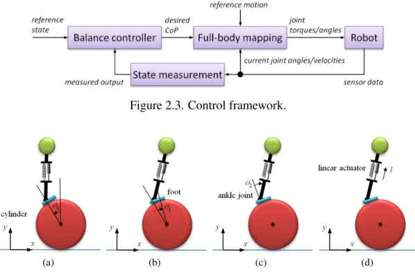
Figure 2.3. Control framework.
(a) (b) (c) (d)
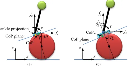
Figure 2.4. Simplified dynamics model of a biped robot with flat feet on a rolling cylinder in the sagittal plane. (a)θ0 is the rolling angle of the cylinder, which also indicates the relative position of the ankle joint to the top of the cylinder if the ankle joint is initially above the top. (b)θ1is the rolling angle of the foot relative to the cylinder. (c)θ2is the angle of the ankle joint, indicating the center of mass (COM) position relative to the ankle. (d)lis the change of the distance.
following discussion, I first derive the linearized equation of motion for each simplified model and then discuss how to design the balance controller and calculate the desired COP from the output of the balance controller.
2.4.1 Flat-Foot Sagittal-Plane Simplified Model
I use a simplified model to characterize the dynamics of the whole system, including the robot and the cylinder, and design a balance control for the system based on the simplified model.
to the ankle joint through a link with a linear actuator on it. The linear actuator is used to model the effect of the knee joint. The configuration of the model can be described by three angular variablesθ0,θ1andθ2 and a linear variablel, as indicated in Fig. 2.4, where θ0 represents the rolling angle of the cylinder (Fig. 2.4a),θ1 denotes the angle of the foot rotating relatively to the cylinder (Fig. 2.4b), andθ2 is the angle of the ankle joint andlis the change in the link length (Fig. 2.4c). Assume that there is no slip between the foot and the cylinder. The positive direction of angles is taken to be clockwise in Fig. 2.4. Letr0,m0, andI0 respectively denote the radius, the mass, and the inertia of the cylinder,m1 andI1 the mass and the inertia of a foot,m2andI2 the mass and inertia of the inverted pendulum, and L=l0+lthe distance between the ankle joint and the lump mass, wherel0 is the distance while the robot is in the rest position. The COM of the foot is assumed to be at the ankle.
The simplified model can be used to characterize the dynamics of the robot standing on the cylinder with both legs or just one leg if the swing leg dynamics is ignored. The linearized equation of motion of the model can be derived as
Mθ¨+Gθ =τ (2.1)
whereθ = [θ0 θ1 θ2 l]T,τ = [0 0 τ f]T,τ is the ankle torque,f is the force from the linear actuator and
M =
M1+I M2+I1 M2 0 M2+I1 M3+I1 M3 0
M2 M3 M3 0
0 0 0 m2
, G=−
G1+m2gl0 m2gl0 m2gl0 0 m2gl0 m2gl0−G1 m2gl0 0 m2gl0 m2gl0 m2gl0 0
0 0 0 0
M1 =m0r20+ 4m1r20+m2L12, M2 =m2l0L1+I2, M3 =m2l20+I2
2.4.2 Geta-Foot Sagittal-Plane Simplified Model
Since it is assumed that the geta foot does not move relatively to the cylinder, the robot can be deemed to be hinged on the cylinder through the ankle joint. Then, the sagittal-plane model has three DOFs in total and one DOF less than the flat-foot model does. The parameters used to describe the motion of the geta-foot model include the rolling angleθ0 of the cylinder, the angleθ2 of the ankle joint, and the lengthlcorresponding to the linear actuator, as indicated in Fig. 2.1.
The linearized equation of motion of the geta-foot sagittal-plane model can be written in the same form as (2.1), whereθ= [θ0 θ2 l]T,τ = [0 τ f]T,τ is the ankle torque,f is the linear actuation force and
M =
M1+I M2 0
M2 M3 0
0 0 m2
, G=−
G1 +m2gL0 m2gL0 0 m2gL0 m2gL0 0
0 0 0
M1 =m0r20+m1(r0+h)2+m2(r0+h+l0)2
M2 =m2l0(r0+h+l0) +I2, M3 =m2l20 +I2
I =I0+I1+I2, G1 = (m1+m2)gh.
2.4.3 Frontal-Plane Simplified Model
Since the cylinder is supposed not to move in the frontal plane, I use a single inverted pendulum model to characterize the motion of the robot alone, as depicted in Fig. 2.1, just like the case that the robot stands on the horizontal ground. Also this model works for either case where flat or geta feet are used. The inverted pendulum model consists of a mobile base representing the COP and a lump mass representing the COM of the robot. The linearized equation of motion of the model is derived as
whereθ= [y θy]T,τ = [fy 0]T, and
M =
m1+m2 m2l0 m2l0 m2l20+I
, G=−
0 0
0 m2l0g .
Here,yis the position of the mobile base,θy is the joint angle,fy is the horizontal input force applied to the mobile base,m1 is the mass of the mobile base,m2 andI are the mass and the inertia of the lump mass, andl0is the length of the inverted pendulum.
2.4.4 Balance Controller for the Sagittal-Plane Motion
Here I discuss the balance controller design for the sagittal plane based on the afore-mentioned simplified models. The balance controller for the frontal plane is given in the next subsection. Recall that there are two simplified models with different feet designs for the sagittal-plane motion. However, the derivations of the balance controller are almost the same, except that the matrices and vectors in the derivation have different dimensions because the two models have different numbers of DOF. Thus I use the flat-foot model as an example hereinbelow to demonstrate how to derive the balance controller.
Equation (2.1) can be rewritten as a state-space differential equation
˙
x=Ax+Bu (2.3a)
y=Cx (2.3b)
wherex= [θT θ˙T]T is the state,u= [τ f]T is the input, and the matricesAandBare given by
A=
04×4 I4×4 −M−1G 04×4
, B =
04×2
M−1 0 0 0 0 1 0 0 1
, C =
I4×4 04×4
Because there is no direct access to the real state of the simplified model, I design an observer to estimate it by comparing the estimated outputyˆand the measured outputy:
˙ˆ
x=Axˆ+Bu+F(y−y)ˆ (2.4)
whereF ∈R8×4 is the observer gain, the estimated outputyˆ=Cxˆ, andxˆis the estimated state. The measured outputyis obtained from the sensor data, which will be discussed in Section 2.5.3.
Referring to the previous work (Yamane and Hodgins, 2009; Zheng and Yamane, 2011, 2013a), I design a state-feedback balance controller as
u=K(x∗−x)ˆ (2.5)
where K ∈ R2×8 is a feedback gain and x∗ is an equilibrium state such thatAx∗ = 0.
The feedback gainK is chosen so that it ensures that all the eigenvalues ofA−BKhave negative real parts and the system asymptotically converges to the equilibrium state. The first and second rows ofK contain the feedback gains for generating the ankle torqueτ and the linear actuation forcef, respectively. SinceAhere has full rank, x∗ =0 is the only equilibrium state of the simplified model.
Combining (2.3)–(2.5), I obtain the following system of the estimated statexˆand the new inputus =y:
˙ˆ
x=Asxˆ+Bsus (2.6a)
ˆ
y=Csxˆ (2.6b)
where
As=A−BK −F C, Bs =F, Cs=C.
2.4.5 Balance Controller for the Frontal-Plane Motion Rewriting (2.2) in the state space yields
˙
x=Ax+Bu (2.7a)
y=Cx (2.7b)
wherex= [y θy y˙ θy˙ ]T is the state,u=fy is the input,y= [y θy]T is the output, and the matricesAandBare given by
A=
02×2 I2×2 −M−1G 0
2×2
, B=
02×1
M−1[1 0]
, C =
I2×2 02×2
.
The observer is given by
˙ˆ
x=Aˆx+Bu+F(U[yCOP yCOM]T −y)ˆ (2.8)
whereU is the matrix given below to convert the measured COP positionyCOPand COM positionyCOMto the configuration of the simplified model,
U =
1 0
−1/l 1/l .
The measurement of the COP and COM positions will be discussed in Section 2.5.
The design of feedback controller is similar to (2.5). Different from the sagittal-plane model as depicted in Fig. 2.2, the inverted pendulum has an infinite number of equilibrium points, which correspond to any case where the COP and the COM of the robot are on the same vertical line. Hence, the feedback controller for the frontal plane is designed as
where yref is the reference COM position and T = [1 0 0 0]T maps yref to the corresponding equilibrium state of the inverted pendulum model.
Combining (2.7)–(2.8), I obtain the following system of the estimated statexˆand input
uf = [yCOP yCOM yref]T:
˙ˆ
x=Afxˆ+Bfuf (2.10a)
ˆ
y=Cfxˆ (2.10b)
where
Af =A−BK−F C, Bf = [F U BKT], Cf =C.
2.4.6 Computation of the Desired COP
From the output of the balance controllers I derive the desired COP, which provides high-level control information and will be used in generating full-body control commands for the robot to maintain balance on the cylinder, as discussed later in Sections 2.6 and 2.7. The y-coordinate (position in the frontal plane) of the desired COP is generated directly in the output of the frontal-plane balance controller. Here I discuss the derivation of the x-andz-coordinates (position in the sagittal plane) of the desired COP from the output of the sagittal-plane balance controller.
The computation of the desired COP in the sagittal plane depends on the adopted sagittal-plane simplified model, i.e., the flat-foot model or the feta-foot model. I start with the case that the simplified model has a flat foot. In this case, the COP is the contact between the foot and the cylinder.
wherex0and z0 are thex- andy-coordinates of the orthogonal projection of the ankle of the simplified model on the sole plane,θˆ1is the foot rotation angle relative to the cylinder obtained from the output of the balance controller, andθ0andθ1are the cylinder rolling angle and the foot rotation angle measured from the real robot, respectively. The determination ofx0,z0,θ0, andθ1will be discussed in the next section together with the measurement of other quantities.
To calculate the desired COP in the case of using the geta-feet model, I first compute the desired force and torque at the ankle joint of the simplified model that are required to realize the motion of the simplified model specified by the balance controller. The desired torqueτ is determined by the feedback controller (2.5). The desired force can be calculated from the desired motion of the lump mass of the simplified model. From the state of the simplified model in the balance controller, the desired acceleration of the lump mass can be derived as
¨
x=r0θ¨0+h(¨θ0cosθ0−θ˙20sinθ0) +l0(¨θ01cosθ01−θ˙012 sinθ01) (2.12a)
¨
z =−h(¨θ0sinθ0+ ˙θ02cosθ0)−l0(¨θ01sinθ01+ ˙θ012 cosθ01) (2.12b)
whereθ01 =θ0+θ1 andθ0,1,θ˙0,1, andθ¨0,1 are obtained from the balance controller (2.6). Then, the desired force can be easily computed by
fx =m2x¨ (2.13a)
fz =m2(¨z+g). (2.13b)
The desired COP can therefore be written as
xCOP =x0+scos ˆθ0 (2.14a)
Table 2.1. Common Sensors used on a Robot and Their Functions
Sensor Function
inertial measurement unit (IMU) global position and orientation of the floating base (hip)
joint angle sensors joint angles
force/torque sensors forces and moments applied by the environment to the ankles
wherex0 andz0 give the orthogonal projection of the ankle in the simplified model on the sole plane,θˆ0is the rolling angle of the cylinder or the inclination angle of the foot specified by the balance controller, andsis the offset of the desired COP from the ankle projection in the sole plane, which can be calculated as
s=−(fxcos ˆθ0−fysin ˆθ0)h+τ fxsin ˆθ0+fycos ˆθ0
(2.15)
wherehis the tooth height of the geta foot andτ is the desired ankle torque obtained from the the feedback controller (2.5) based on the simplified model.
2.5 System Measurement
(a) (b)
Figure 2.5. Measurement of the actual COP and the state of (a) the flat-feet model or (b) the geta-feet model.
2.5.1 COM Measurement
It is straightforward to measure the actual COM position of the robot. Based on the data from the IMU and joint angle sensors, the COM position can be easily calculated through forward kinematics using the available kinematic and dynamic models of the robot. By doing this, I also obtain the global position and orientation of each foot of the robot.
2.5.2 COP Measurement
(Fig. 2.5b). The COP plane can be expressed as x y z = x0 y0 z0 +
cosα 0
0 1
−sinα 0
u v (2.16)
where[x0 y0 z0]T is an arbitrary point on the plane andαis the inclination angle of the plane, both of which can be determined from the positions and orientations of feet. To determine the point, the average position of two feet is used, while their average orientation is used to determine the inclination angle. The COP plane determined in this way tries to fit both feet, which may not perfectly align with each other on the cylinder.
From force/torque sensor data, I obtain the contact force and moment applied at each foot. Based on the global positions and orientations of feet, I can convert the forces and moments on both feet to the net forcef and momentnapplied to the robot with respect to the global frame. Then, the actual COP should satisfy the following equation
cosα 0 −sinα
0 1 0
(n+ ˆf x y z
) = 0 (2.17)
wherefˆrepresents the cross product and[x y z]T is the actual COP position with respect to the global frame.
Substituting (2.16) into (2.17) yields
A u v
where
A=
cosα 0 −sinα
0 1 0
ˆ f
cosα 0
0 1
−sinα 0
(2.19)
b =−
cosα 0 −sinα
0 1 0
(n+ ˆf x0 y0 z0
). (2.20)
Finally, solving (2.18) foruandvand substituting them into (2.16), I obtain the measured position of the actual COP in the global frame.
2.5.3 Configuration Measurement of the Simplified Models
In the frontal plane, the actual COM and COP positions are used directly as the input to the balance controller (2.10). As for the input to the balance controller in the sagittal plane, however, I need to measure the actual configuration of the simplified model from the robot, which is explained as follows.
For the flat-foot model, I first calculate the distancedfrom the orthogonal projection of the ankle on the COP plane to the actual COP in the sagittal plane, as shown in Fig. 2.5a. Then, the measured value of angleθ1is equal tod/r0and that of angleθ0is equal toα−d/r0, wherer0 is the radius of the cylinder. Finally, from the actual COM position relative to the ankle position, I can easily calculate the actual values ofθ2andl.
The configuration measurement of the geta-foot model is the same as that of the flat-foot model except that the rolling angleθ0of the cylinder is taken directly to be the inclination angle of robot feet.
Table 2.2. Measurement of Quantities
Quantity Required Sensor Data
robot feet positions/orientations forward kinematics based on the IMU and joint sensor data
actual COM position forward kinematics based on the IMU and joint sensor data
actual COP position force/torque sensor data and robot feet positions/ori-entations
inclination angle of the COP plane
robot feet orientations ankle position of the simplified
model
robot feet positions/orientations ankle projection on the COP
plane
robot feet positions/orientations
rolling angleθ0 robot feet positions/orientations and actual COP position (flat-feet model)
robot feet orientations (geta-feet model)
foot rotation angleθ1 robot feet positions/orientations and actual COP position (only for the flat-feet model)
ankle joint angleθ2 ankle position of the simplified model, actual COM position, and inclination angle of the COP plane length changel ankle and COM positions
2.6 Full-Body Mapping and Simulation
The desired COP obtained from the balance controllers only tells the high-level in-formation for maintaining the balance of the robot on the cylinder. To actually control the robot, full-body control commands need to be determined. Assume that the robot in simulation uses torque control, which means that the robot takes joint torques as the actual command to activate and control its motion. Here I discuss how to compute the joint torques for controlling the robot to follow the desired COP and maintain balance on the cylinder, followed by simulation results.
2.6.1 Torque Mapping
cylinder’s motion, I extend the method to including the cylinder with the robot and consider their dynamics all together.
The dynamics of the whole system, including the robot and the cylinder, can be described by the following equation
Mr 0
0 Mc
¨ qr ¨ qc + cr cc =
NTτ
0 + JT r 0 JT c1 Jc2T
f1 f2
. (2.21)
where Mr and Mc are the joint-space inertia matrices of the robot and the cylinder, re-spectively,cr and ccare the sums of Coriolis, centrifugal and gravity forces for them,τ comprises the joint torques and N is the matrix used to map the joint torques into the generalized forces, f1 comprises the contact forces/moments between the robot and the cylinder andJr and Jc1 are the Jacobian matrices whose transposes convert f1 into the generalized forces for the robot and the cylinder, respectively, andf2comprises the contact force/moment between the cylinder and the ground andJc2 is the Jacobian matrix whose transpose mapsf2into the generalized forces for the cylinder.
The goal of the method (Yamane and Hodgins, 2009) is to compute the joint torques for the robot to realize the desired COP as well as the desired joint accelerationsqˆ¨and the desired foot accelerationsrˆ¨for achieving a given reference motion. In the case herein, the reference motion for the robot consists merely of a single full-body standing pose on the cylinder. The desired accelerations of joints, including the joints of both the robot and the cylinder, are determined by the traditional proportional-derivative control law as
ˆ ¨
q = ¨qref +kd( ˙qref −q˙) +kp(qref −q) (2.22)
The desired accelerationsˆ¨rof robot’s feet, consisting of linear and angular components, are determined using the same control law as (2.22).
However, tracking the desired COP and realizing the reference pose may conflict with each other. Hence, an optimization problem is formulated to compute the joint torques that respect both of them. Free variables of the optimization problem include joint torquesτ
and contact forcesf, while joint accelerationsq¨depend completely onτ andf according to the full-body dynamics equation (2.21). The cost function to be minimized consists of several terms addressed as below.
The COP error, namely the error in tracking the desired COP obtained from the balance controller, can be expressed as the magnitude of the resultant moment around the desired COP as
ZCOP =
1 2f
T 1 P
TW
PP f1 (2.23)
whereP is the matrix that mapsf1 to the resultant moment around the desired COP. The errorZqfrom the desired joint accelerations can be written as
Zq=
1
2(ˆq¨−q)¨
TW
q(ˆq¨−q)¨ . (2.24)
From (2.21) it follows that the joint accelerationsq¨can be expressed as a linear function of
τ andf.
The errorZτ from the desired feet accelerations can be written as
Zc =
1
2(ˆr¨−r)¨
TW
c(ˆ¨r−r)¨ (2.25)
whereˆ¨ris the desired feet accelerations and can be determined using the same control law as (2.22). The relationship between the generalized velocityq˙and the velocity of one foot
˙
ri is given by
˙
Differentiating (2.26) yields the foot acceleration:
¨
r =Jrq¨r+ ˙Jq˙r. (2.27)
From (2.21) and (2.27),r¨is completely determined byτ andf.
Other terms may include the magnitudes of joint torques and contact forces:
Zm =
1 2τ
TW ττ +
1 2f
TW
ff. (2.28)
Combining all the terms, the cost function can be written in a quadratic form
Z = 1 2y
TAy+yTb+c (2.29)
wherey = τT fTT. The analytic solution to the optimization problem (2.29) isy =
−A−1b. Then the resulting optimized joint torquesτ are sent to the robot as depicted in Fig. 2.3.
2.6.2 Simulation
I use the dynamics simulator with rigid-contact model developed by the University of Tokyo (Yamane and Nakamura, 2008a,b) to conduct my simulation. The simulator computes the actual contact forces and joint accelerations after applying the optimized joint torques obtained as above to the robot, considering the complementary constraint on the contact force and the contact link motion. This problem can be formulated as a linear complementary problem and solved by the algorithm developed by Yamane and Nakamura (2008b). This is out of the scope of this dissertation and readers are referred to the relevant publications.
(a) (b)
Figure 2.6. Simulation of a biped robot with (a) flat feet or (b) geta feet on a rolling cylinder. The blue arrow represents the external disturbance applied to the robot.
roll, yaw at the shoulder and pitch at the elbow) and fix wrist joints. There are 3 joints in the torso. The robot model is about 1.7 meters tall and 65 kg in weight. The radius of the cylinder is 0.254 m.
Both flat and geta feet are tested in simulation, as shown in Fig. 2.6. A disturbing force is applied at the hip of robot in the sagittal plane to verify the effectiveness of the balance controller. In the case of flat feet, the robot can successfully balance on the cylinder under a disturbing force of 20 N applied for 100 ms. It is noticed in simulation that it is hard for the robot to completely stop on top of the cylinder and immobilize the cylinder. In the case of geta feet, by contrast, the robot can survive under a bigger disturbance, a 40 N force applied for 100 ms, and freeze on the cylinder. This is due to that the robot has a much bigger support region and the model has one less DOF by using this special design of feet. A video of the simulation can be found on http://www.cs.unc.edu/˜yuzheng/ dissertation/.
2.7 Experiments on the Sarcos Humanoid Robot
Figure 2.7. Experimental setup on the Sarcos humanoid robot.
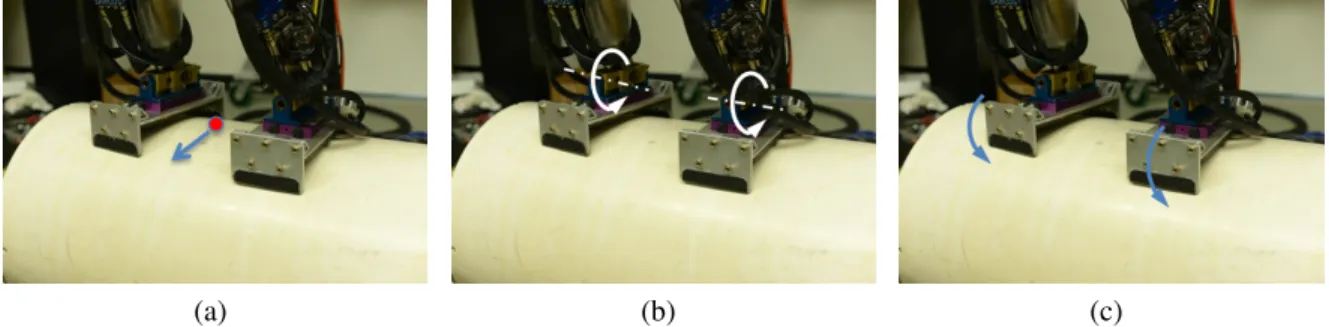
required in computing the joint torques. Hence, I switch to the position control and compute the desired joint angles for the robot in order to maintain balance. Moreover, from the simulation results it has been seen that it is easier for the robot to stand on the cylinder using geta feet. Thus, I use geta feet rather than flat feet in the experiment. By doing this, it also becomes easier for the robot to reach an initial pose that is close to the static equilibrium.
The key idea of the position mapping is to convert the desired COP change to the desired joint angles for the robot. Fig. 2.8 illustrates this conversion. Suppose that the desired COP needs to move forward in comparison with the current COP, as depicted in Fig. 2.8a. This is equivalent to increasing the ankle torque (Fig. 2.8b) or to extending the feet (Fig. 2.8c). Therefore, I can convert the desired COP to the change of the foot orientation by the following law:
u= (xdCOP−x0COP) +Kpe(t) +Ki Z t
0
e(τ)dτ +Kd d
(a) (b) (c)
Figure 2.8. Conversion of the desired COP to the foot rotation. (a) The desired COP moving forward. (b) Increasing the ankle torque in the direction as shown. (c) Extending the feet.
where xd
COP and x0COP are the desired and initial positions of the COP in the sagittal plane, respectively, e(t)is the error between the desired COP and the actual COP, and Kp, Ki, andKd are the proportional, integral, and derivative gains. Finally, I take u/R as the desired rotation of feet from their initial orientation, whereR is a value that needs to be tuned in the experiment. With proper settings of Kp, Ki, Kd, and R, the Sarcos humanoid robot can balance on the cylinder. A video showing the experiment is provided onhttp://www.cs.unc.edu/˜yuzheng/dissertation/.
2.8 Conclusions and Future Work
technique. I also conduct hardware experiments on a position-controlled robot and use a joint angle mapping instead of joint torque optimization. The robot can balance on a free-rolling cylinder for at least 20 s.
CHAPTER 3: MANIPULATING A DYNAMIC OBJECT BY ACTIVE WALKING
3.1 Introduction
Only being able to balance on the cylinder will get the robot nowhere. In order to enhance its mobility, the robot need be able to actively move the cylinder in some way. Based on the balance controller presented in the previous chapter, this chapter discusses how the robot can actively manipulate the rolling of the cylinder through biped walking on top of it, which is challenging even for normal humans.
3.1.1 Main Results
In this chapter, I present two methods for generating biped walking gaits for a humanoid robot to walk on and roll the cylinder. In the first method, I allow the walking gait to have a double-support phase, in which both robot feet are in contact with the cylinder. The rolling of the cylinder happens only during the double-support phase, whereas in the single-support phase the robot stands still on one foot and takes a step on the cylinder. Hence, the stepping motion of the swing foot and the rotation of the cylinder happen in sequence. Since there is a pause between steps and the cylinder does not roll continuously, this method generates an intermittent walking behavior. Also, having the double-support phase, the COP can gradually shift from the left side to the right or vice versa, which does not require a fast COM motion and makes the walking gait more static and easier for the robot to realize.
keeps rolling without a stop between steps. Thus, the generated walking behavior is more continuous. Furthermore, I expect the walking gait to be identical between steps in terms of the states of the robot and the cylinder, and such a gait is called a cyclic walking gait.
3.1.2 Organization
This chapter is organized as follows. Section 3.2 summarizes the previous work on biped walking generation. Sections 3.3 and 3.4 discuss the generating of the static walking gait and the cyclic walking gait, respectively. Conclusions and future work are given in Section 3.5.
3.2 Previous Work
3.2.1 Biped Locomotion Generation
Hirukawa et al. (2006) used a more general criterion based on feasible contact forces in the design of a walking pattern generator.
Humanoid locomotion can also be generated in a reverse way. One may first have a reference COM or upper-body motion for a humanoid robot, which can be acquired from a captured human motion or a motion planner. Then, based on a simplified dynamics model, the required COP trajectory can be quickly computed from the reference motion. From the COP trajectory, a sequence of appropriate footsteps can be determined to cover it. Finally, the full-body trajectories in terms of joint angles for the robot can be calculated through inverse kinematics based on the COM or upper body motion and the sequence of footsteps. Nevertheless, there is not much work on this kind of approaches (Sugihara, 2008).
3.2.2 Limit Cycle Walking of Passive Walkers
Limit cycle walking is a fundamental topic in the research of passive biped robots. McGeer (1990) first demonstrated that a passive biped robot can walk down a slope in a steady periodic gait without any active control. The only energy supply to the robot is the potential energy, which compensates the loss of energy when the swing leg hits the ground. After McGeer’s pioneering work, many researchers investigated passive biped walking. Goswami et al. (1998) and Garcia et al. (1998) verified the existence and the stability of limit cycles. Osuka and Kirihara (2000) first demonstrated this symmetric motion on a real passive robot. Collins et al. (2001) built the first three-dimensional passive biped robot with knees. Ikemata et al. (2003; 2008) studied several factors that may affect the stability of a limit cycle, such as the support exchange, the stabilization of a fixed point, and the motion of the swing leg. Freidovich et al. (2009) proposed a faster way to seek both stable and unstable limit cycles than traditional numerical routines.
ground and have higher capability to handle disturbances. One energy-efficient way to add actuation is the use of actuated ankles (Kuo, 2002; Collins et al., 2005; Hobbelen and Wisse, 2008a,b; Franken et al., 2008). Using the ankle push-off not only decreases the energy use (Kuo, 2002; Collins et al., 2005) but also increases limit cycle walkers’ ability to reject disturbances (Hobbelen and Wisse, 2008a). The use of ankle actuation also allows a robot to achieve different walking speed in limit cycle walking (Hobbelen and Wisse, 2008b). It has also been shown with simulation that pushing off before the swing leg hits the ground is energetically more efficient than pushing off after the heel strikes (Franken et al., 2008). Actuation can also be added at the hip joint (Dertien, 2006). Harada et al. (2010) applied the limit cycle based walking generation to a model of present humanoid robots with more active joints and flat feet.
3.3 Static Walking Gait Generation
In this section, I discuss how to generate a walking gait simply based on the balance controller presented in the previous chapter. It is expected that, by using the balance controller, the robot will roll the cylinder to recover its feet to be horizontal once the feet lean on top of the cylinder. Then, I use this property to design a walking gait generator and enable the robot to intensionally roll the cylinder by changing foot locations on top of it. Fig. 3.1 depicts a framework for the walking gait generator, which consists primarily of planners for frontal and sagittal motions and the balance controller. The frontal and sagittal motion planners generate the trajectories of the COM and the feet so that the full-body reference motion, expressed as joint trajectories, can be calculated through inverse kinematics.
3.3.1 Frontal Motion Planner
Figure 3.1. Framework for walking motion generation on a rolling cylinder.
the supporting foot and the swing foot can lift up. Yamane and Hodgins (2010) proposed a method to modify the COM trajectory of a reference motion such that the corresponding desired COP can stay within the support region. I use this method to generate the reference COM trajectory in the frontal plane. Following the method (Yamane and Hodgins, 2010), I first discretize the state-space equation of the balance controller (2.10) and obtain
xk+1 =Axk+Buk (3.1)
where xk is the state and uk is the input at sampling time k. In contrast to the balance controller (2.10), here I do not include the observer in (3.1) because I am planning the motion and do not have real measurements. As a result,ukcomprises only a COM position. The output is chosen to be the COP position and can be written as
yk =Cxk (3.2)
Figure 3.2. Framework for sagittal walking motion generation on a rolling cylinder.
Given an initial state x0 and the COM positions for the next n frames, uk (k =
0,1, . . . , n−1), through (3.1) I can predict the COP position innframes by
yn =C(Anx0+M u) (3.3)
where
M =An−1B An−2B · · · B, u= [u0 u1 · · ·un−1] T
. (3.4)
Suppose that yref is the desired COP position in n frames. Then, I can compute a reference COM trajectoryufor thenframes such thatyn approachesyref by minimizing the following cost function:
Zd =
1
2(yref −yn)
2+ 1
2( ˆu−u)
T
W ( ˆu−u) (3.5)
whereuˆis a nominal COM trajectory and can be simply taken to beukˆ =x0+k(yres−x0)/n. The purpose of the first term ofZdis to bring the COP as close as possible to the desired valueyref, while that of the second term is to prevent the generated COM trajectory deviating from a reasonable region.
3.3.2 Sagittal Motion Planner
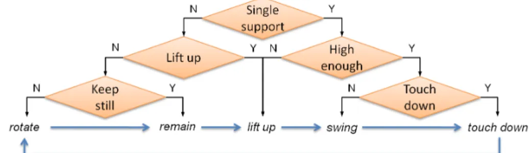
The robot undergoes the double support phase and the single support phase alternately on the cylinder. The foot to be lifted up and put down at a different location is called the swing foot, while the other foot that supports the robot is called the supporting foot. The swing foot will have one of the following five actual/desired states:
a) keeping contact with the cylinder and rotating together with the supporting foot to roll the cylinder;
b) remaining at its current position and orientation while the COP moves to the side of the supporting foot;
c) lifting up while the supporting foot keeps still on the cylinder;
d) swinging to the target position for touching down;
e) touching down at the target position on the cylinder.
The swing foot needs to follow the desired states in the sequence as shown in Fig. 3.2 in order to accomplish a walking step. After the swing foot lands on the cylinder, it becomes the new supporting foot and the supporting foot becomes the new swing foot for the next step. For different desired states, corresponding reference motions are generated and used in computing joint torques as discussed in Section 2.6.1. Note that the actual state of a foot may not immediately match the desired one. In what follows, I discuss the generation of reference motion for each desired state and the condition for triggering a desired state.
Figure 3.3. Illustration of the motion of the swing foot in a step. The swing foot (in the blue color) (a) rotates together with the supporting foot (not shown) and rolls the cylinder for angleα, (b) lifts up, (c) moves backwards, and then (d) touches down. Once touching down, the swing foot becomes the supporting foot (in the green color) for the next step and (e) rotates and rolls the cylinder for another angleα. (a) and (e) happen at the same time in one step on the swing foot and the supporting foot, respectively.
can be known directly from the state that has just happened, and it is only required to check if the corresponding condition is triggered.
Fig. 3.3 illustrates the motion of the swing foot in one step. Assume that the cylinder is required to roll forward for an angleαin every step. At the beginning of a step, the swing foot, namely the supporting foot in the previous step, should be on top of the cylinder, while the supporting foot, namely the swing foot after touching down at the end of the previous step, is behind the top. To make the supporting and swing feet rotate about the cylinder, which as a result causes the cylinder to roll, I first measure the state of the simplified model based only on the position and orientation of the supporting foot and use the measured state as the input to the balance controller. Since the supporting foot is behind the top of the cylinder, the balance controller should be able to bring it to the top, as shown by arrow (e) in Fig. 3.3, which causes the cylinder to roll forward due to the friction between the foot and the cylinder. The swing foot can rotate simultaneously with the supporting foot and the cylinder as long as it remains in contact with the cylinder.