Lecture 5
Basic theorems of Probability Theory
Plan of the lecture: 1. Probability laws
1.1 Discrete Probability Law 1.2 Continuous Models
1.3 Properties of Probability Laws 2. Conditional probability
2.1 Definition of conditional probability
2.2 Conditional Probabilities Specify a Probability Law 2.3 Using Conditional Probability for Modeling
3. Total probability theorem and Bayes` rule 4. Independence
5. Reliability
6. Independent Trials and the Binomial Probabilities
1 Probability laws
Suppose we have settled on the sample space 𝛺 associated with an experiment. Then, to complete the probabilistic model, we must introduce a probability law. Intuitively, this specifies the “likelihood” of any outcome, or of any set of possible outcomes (an event, as we have called
it earlier). More precisely, the probability law assigns to every event 𝐴, a number 𝑃(𝐴), called the probability of 𝐴, satisfying the Probability Axioms.
In order to visualize a probability law, consider a unit of mass which is to be “spread” over the sample space. Then, 𝑃(𝐴) is simply the total mass that was assigned collectively to the elements of 𝐴. In terms of this analogy, the additivity axiom becomes quite intuitive: the total mass in a sequence of disjoint events is the sum of their individual masses.
A more concrete interpretation of probabilities is in terms of relative frequencies: a statement such as 𝑃(𝐴) = 2/3 often represents a belief that event 𝐴 will materialize in about two thirds out of a large number of repetitions of the experiment. Such an interpretation, though not always appropriate, can sometimes facilitate our intuitive understanding.
There are many natural properties of a probability law which have not been included in the Axioms for the simple reason that they can be derived from them. For example, note that the normalization and additivity axioms imply that
1 = 𝑃 Ω = 𝑃 Ω ∪ ∅ = 𝑃 Ω + 𝑃 ∅ = 1 + 𝑃 ∅ ,
and this shows that the probability of the empty event is 0:
𝑃 ∅ = 0.
As another example, consider three disjoint events 𝐴1, 𝐴2, and 𝐴3. We can use the additivity axiom for two disjoint events repeatedly, to obtain
𝑃 𝐴1∪ 𝐴2∪ 𝐴3 = 𝑃 𝐴1∪ 𝐴2 ∪ 𝐴3 = 𝑃 𝐴1 + 𝑃 𝐴2∪ 𝐴3 = 𝑃 𝐴1 + 𝑃 𝐴2 + 𝑃 𝐴3 .
Proceeding similarly, we obtain that the probability of the union of finitely many disjoint events is always equal to the sum of the probabilities of these events. More such
1.1 Discrete Probability Law
If the sample space consists of a finite number of possible outcomes, then the probability law is specified by the probabilities of the events that consist of a single element. In particular, the probability of any event {𝑠1, 𝑠2, … , 𝑠𝑛} is the sum of the probabilities of its elements:
𝑃 {𝑠1, 𝑠2, … , 𝑠𝑛} = 𝑃 {𝑠1} + 𝑃 {𝑠2} + ⋯ + 𝑃 {𝑠𝑛} .
In the special case where the probabilities 𝑃 {𝑠1} , … , 𝑃 {𝑠𝑛} are all the same (by necessity equal to 1/𝑛, in view of the normalization axiom), we obtain the following.
Discrete Uniform Probability Law
If the sample space consists of 𝑛 possible outcomes which are equally likely (i.e., all single-element events have the same probability), then the probability of any event 𝐴is given by
𝑃(𝐴) =𝑁𝑢𝑚𝑏𝑒𝑟 𝑜𝑓 𝑒𝑙𝑒𝑚𝑒𝑛𝑡𝑠 𝑜𝑓 𝐴𝑛 .
1.2 Continuous Models
Probabilistic models with continuous sample spaces differ from their discrete counterparts in that the probabilities of the single-element events may not be sufficient to characterize the probability law. This is illustrated in the following example, which also illustrate how to generalize the uniform probability law to the case of a continuous sample space.
Example 1. A wheel of fortune is continuously calibrated from 0 to 1, so the possible outcomes of an experiment consisting of a single spin are the numbers in the interval 𝛺 = [0, 1]. Assuming a fair wheel, it is appropriate to consider all outcomes equally likely, but what is the probability of the event consisting of a single element? It cannot be positive, because then, using the additivity axiom, it would follow that events with a sufficiently large number of elements would have probability larger than 1. Therefore, the probability of any event that consists of a single element must be 0. In this example, it makes sense to assign probability 𝑏 − 𝑎 to any subinterval [𝑎, 𝑏] of [0, 1], and to calculate the probability of a more complicated set by evaluating its “length”. This assignment satisfies the three probability axioms and qualifies as a legitimate probability law.
The first to arrive will wait for 15 minutes and will leave if the other has not yet arrived. What is the probability that they will meet?
Let us use as sample space the square 𝛺 = [0, 1] × [0, 1], whose elements are the possible pairs of delays for the two of them. Our interpretation of “equally likely” pairs of delays
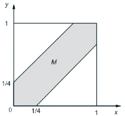
is to let the probability of a subset of 𝛺 be equal to its area. This probability law satisfies the three probability axioms. The event that Romeo and Juliet will meet is the shaded region in Fig. 1, and its probability is calculated to be 7/16.
Fig. 1: The event 𝑀that Romeo and Juliet will arrive within 15 minutes of each other (cf.
Example 2) is 𝑀 = 𝑥, 𝑦 | 𝑥 − 𝑦 ≤14, 0 ≤ 𝑥 ≤ 1, 0 ≤ 𝑦 ≤ 1 , and is shaded in the figure.
The area of 𝑀 is 1 minus the area of the two unshaded triangles, or 1 − (3/4)(3/4) = 7/16. Thus, the probability of meeting is 7/16.
1.3 Properties of Probability Laws
Probability laws have a number of properties, which can be deduced from the axioms. Some of them are summarized below.
Some Properties of Probability Laws
Consider a probability law, and let 𝐴, 𝐵, and 𝐶be events. (a) If A ⊂ B, then P(A) ≤ P(B).
(b) 𝑃(𝐴 ∪ 𝐵) = 𝑃(𝐴) + 𝑃(𝐵) − 𝑃(𝐴 ∩ 𝐵). (c) 𝑃(𝐴 ∪ 𝐵) ≤ 𝑃(𝐴) + 𝑃(𝐵).
(d) 𝑃(𝐴 ∪ 𝐵 ∪ 𝐶) = 𝑃(𝐴) + 𝑃(𝐴𝑐 ∩ 𝐵) + 𝑃(𝐴𝑐∩ 𝐵𝑐∩ 𝐶).
Fig. 2
2 Conditional probability
2.1 Definition of conditional probability
Conditional probability is the probability of some event 𝐴, given the occurrence of some other event 𝐵. Conditional probability is written 𝑃(𝐴|𝐵), and is read “the probability of 𝐴, given 𝐵”.
Joint probability is the probability of two events in conjunction. That is, it is the
probability of both events together. The joint probability of 𝐴 and 𝐵 is written 𝑃(𝐴 ∩ 𝐵) or
𝑃(𝐴, 𝐵).
Marginal probability is then the unconditional probability 𝑃(𝐴) of the event 𝐴; that is, the probability of 𝐴, regardless of whether event 𝐵 did or did not occur. If 𝐵 can be thought of as the event of a random variable 𝑋 having a given outcome, the marginal probability of 𝐴 can be obtained by summing (or integrating, more generally) the joint probabilities over all
outcomes for 𝑋. For example, if there are two possible outcomes for 𝑋 with corresponding events 𝐵 and 𝐵′, this means that 𝑃 𝐴 = 𝑃 𝐴 ∩ 𝐵 + 𝑃(𝐴 ∩ 𝐵′). This is called marginalization.
Conditional probability provides us with a way to reason about the outcome of an experiment, based on partial information. Here are some examples of situations we have in mind:
In a word guessing game, the first letter of the word is a “t”. What is the likelihood that the second letter is an “h”?
How likely is it that a person has a disease given that a medical test was negative?
A spot shows up on a radar screen. How likely is it that it corresponds to an aircraft? In more precise terms, given an experiment, a corresponding sample space, and a probability law, suppose that we know that the outcome is within some given event 𝐵. We wish to quantify the likelihood that the outcome also belongs to some other given event 𝐴. We thus seek to construct a new probability law, which takes into account this knowledge and which, for any event 𝐴, gives us the conditional probability of 𝐴given 𝐵, denoted by 𝑃(𝐴|𝐵).
We would like the conditional probabilities 𝑃(𝐴|𝐵) of different events 𝐴 to constitute a legitimate probability law, that satisfies the probability axioms. They should also be consistent with our intuition in important special cases, e.g., when all possible outcomes of the experiment are equally likely. For example, suppose that all six possible outcomes of a fair die roll are equally likely. If we are told that the outcome is even, we are left with only three possible outcomes, namely, 2, 4, and 6. These three outcomes were equally likely to start with, and so they should remain equally likely given the additional knowledge that the outcome was even. Thus, it is reasonable to let
𝑃(𝑡ℎ𝑒 𝑜𝑢𝑡𝑐𝑜𝑚𝑒 𝑖𝑠 6 | 𝑡ℎ𝑒 𝑜𝑢𝑡𝑐𝑜𝑚𝑒 𝑖𝑠 𝑒𝑣𝑒𝑛) =13.
This argument suggests that an appropriate definition of conditional probability when all outcomes are equally likely, is given by
𝑃(𝐴|𝐵) = 𝑛𝑢𝑚𝑏𝑒𝑟 𝑜𝑓 𝑒𝑙𝑒𝑚𝑒𝑛𝑡𝑠 𝑜𝑓 𝐴∩𝐵𝑛𝑢𝑚𝑏𝑒𝑟 𝑜𝑓 𝑒𝑙𝑒𝑚𝑒𝑛𝑡𝑠 𝑜𝑓 𝐵 .
Generalizing the argument, we introduce the following definition of conditional probability:
𝑃(𝐴|𝐵) =𝑃(𝐴∩𝐵)𝑃(𝐵) ,
2.2 Conditional Probabilities Specify a Probability Law
For a fixed event 𝐵, it can be verified that the conditional probabilities 𝑃(𝐴|𝐵) form a legitimate probability law that satisfies the three axioms. Indeed, nonnegativity is clear. Furthermore,
𝑃(𝛺|𝐵) =𝑃(𝛺∩𝐵)𝑃(𝐵) = 𝑃(𝐵)𝑃(𝐵)= 1,
and the normalization axiom is also satisfied. In fact, since we have 𝑃(𝐵|𝐵) = 𝑃(𝐵)/𝑃(𝐵) = 1, all of the conditional probability is concentrated on 𝐵. Thus, we might as well discard all possible outcomes outside 𝐵 and treat the conditional probabilities as a probability law defined on the new universe 𝐵.
To verify the additivity axiom, we write for any two disjoint events 𝐴1 and 𝐴2,
𝑃 𝐴1∪ 𝐴2 𝐵 =𝑃 𝐴1𝑃 𝐵 ∪𝐴2 ∩𝐵 =𝑃 𝐴1∩𝐵 ∪ 𝐴𝑃 𝐵 2∩𝐵 =𝑃 𝐴1∩𝐵 +𝑃 𝐴𝑃 𝐵 2∩𝐵 =𝑃 𝐴𝑃 𝐵 1∩𝐵 +𝑃 𝐴𝑃 𝐵 2∩𝐵 =
𝑃(𝐴1|𝐵) + 𝑃(𝐴2|𝐵),
where for the second equality, we used the fact that 𝐴1∩ 𝐵 and 𝐴2∩ 𝐵 are disjoint sets, and for the third equality we used the additivity axiom for the (unconditional) probability law. The argument for a countable collection of disjoint sets is similar.
Since conditional probabilities constitute a legitimate probability law, all general properties of probability laws remain valid. For example, a fact such as 𝑃(𝐴 ∪ 𝐶) ≤ 𝑃(𝐴) +
𝑃(𝐶) translates to the new fact 𝑃(𝐴 ∪ 𝐶|𝐵) ≤ 𝑃(𝐴|𝐵) + 𝑃(𝐶|𝐵).
Example. We toss a fair coin three successive times. We wish to find the conditional probability 𝑃(𝐴|𝐵) when 𝐴and 𝐵are the events
𝐴 = {𝑚𝑜𝑟𝑒 ℎ𝑒𝑎𝑑𝑠 𝑡ℎ𝑎𝑛 𝑡𝑎𝑖𝑙𝑠 𝑐𝑜𝑚𝑒 𝑢𝑝}, 𝐵 = {1𝑠𝑡 𝑡𝑜𝑠𝑠 𝑖𝑠 𝑎 ℎ𝑒𝑎𝑑}.
The sample space consists of eight sequences,
𝛺 = {𝐻𝐻𝐻, 𝐻𝐻𝑇, 𝐻𝑇𝐻, 𝐻𝑇𝑇, 𝑇𝐻𝐻, 𝑇𝐻𝑇, 𝑇𝑇𝐻, 𝑇𝑇𝑇},
which we assume to be equally likely. The event 𝐵 consists of the four elements 𝐻𝐻𝐻, 𝐻𝐻𝑇,
𝑃(𝐵) = 48.
The event 𝐴 ∩ 𝐵 consists of the three elements outcomes 𝐻𝐻𝐻, 𝐻𝐻𝑇, 𝐻𝑇𝐻, so its probability is
𝑃(𝐴 ∩ 𝐵) = 38.
Thus, the conditional probability 𝑃(𝐴|𝐵) is
𝑃 𝐴 𝐵 =𝑃 𝐴∩𝐵 𝑃 𝐵 =3 84 8 =34.
Because all possible outcomes are equally likely here, we can also compute 𝑃(𝐴|𝐵) using a shortcut. We can bypass the calculation of 𝑃(𝐵) and 𝑃(𝐴 ∩ 𝐵), and simply divide the number of elements shared by 𝐴 and 𝐵 (which is 3) with the number of elements of 𝐵 (which is 4), to obtain the same result 3/4.
2.3 Using Conditional Probability for Modeling
When constructing probabilistic models for experiments that have a sequential character, it is often natural and convenient to first specify conditional probabilities and then use them to determine unconditional probabilities. The rule 𝑃(𝐴 ∩ 𝐵) = 𝑃(𝐵)𝑃(𝐴|𝐵), which is a restatement of the definition of conditional probability, is often helpful in this process.
We have a general rule for calculating various probabilities in conjunction with a tree-based sequential description of an experiment. In particular:
We set up the tree so that an event of interest is associated with a leaf. We view the
occurrence of the event as a sequence of steps, namely, the traversals of the branches along the path from the root to the leaf.
We record the conditional probabilities associated with the branches of the tree.
We obtain the probability of a leaf by multiplying the probabilities recorded along the
corresponding path of the tree.
is viewed as an occurrence of 𝐴1, followed by the occurrence of 𝐴2, then of 𝐴3, etc, and it is visualized as a path on the tree with 𝑛 branches, corresponding to the events 𝐴1, …, 𝐴𝑛. The probability of 𝐴is given by the following rule (see also Fig. 3).
Fig. 3
Multiplication Rule
Assuming that all of the conditioning events have positive probability, we have
𝑃 𝑛𝑖=1𝐴𝑖 = 𝑃(𝐴1)𝑃(𝐴2|𝐴1)𝑃(𝐴3|𝐴1∩ 𝐴2) ⋯ 𝑃 𝐴𝑛| 𝑛−1𝑖=1 𝐴𝑖 .
The multiplication rule can be verified by writing
𝑃 𝑛𝑖=1𝐴𝑖 = 𝑃(𝐴1)𝑃(𝐴𝑃(𝐴1)1∩𝐴2)𝑃(𝐴𝑃(𝐴1∩𝐴2)1∩𝐴2∩𝐴3)⋯𝑃 𝐴𝑖 𝑛 𝑖=1 𝑃 𝑛 −1𝑖=1 𝐴𝑖 ,
and by using the definition of conditional probability to rewrite the right-hand side above as
𝑃(𝐴1)𝑃(𝐴2|𝐴1)𝑃(𝐴3|𝐴1∩ 𝐴2) ⋯ 𝑃 𝐴𝑛| 𝑛−1𝑖=1 𝐴𝑖 .
For the case of just two events, 𝐴1 and 𝐴2, the multiplication rule is simply the definition of conditional probability.
3 Total probability theorem and Bayes` rule
Let`s explore some applications of conditional probability. We start with the following theorem, which is often useful for computing the probabilities of various events, using a “divide-and-conquer” approach.
Let 𝐴1, …, 𝐴𝑛 be disjoint events that form a partition of the sample space (each possible outcome is included in one and only one of the events 𝐴1, …, 𝐴𝑛) and assume that 𝑃(𝐴𝑖) > 0, for all 𝑖 = 1, … , 𝑛. Then, for any event 𝐵, we have
𝑃(𝐵) = 𝑃(𝐴1∩ 𝐵) + ⋯ + 𝑃(𝐴𝑛 ∩ 𝐵) = 𝑃(𝐴1)𝑃(𝐵|𝐴1) + ⋯ + 𝑃(𝐴𝑛)𝑃(𝐵|𝐴𝑛).
The theorem is visualized and proved in Fig. 4. Intuitively, we are partitioning the sample space into a number of scenarios (events) 𝐴𝑖. Then, the probability that 𝐵 occurs is a weighted average of its conditional probability under each scenario, where each scenario is weighted according to its (unconditional) probability. One of the uses of the theorem is to compute the probability of various events 𝐵 for which the conditional probabilities 𝑃(𝐵|𝐴𝑖) are known or easy to derive. The key is to choose appropriately the partition 𝐴1, …, 𝐴𝑛, and this choice is often suggested by the problem structure.
Fig. 4
Visualization and verification of the total probability theorem (fig. 4). The events 𝐴1, …,
𝐴𝑛 form a partition of the sample space, so the event 𝐵 can be decomposed into the disjoint
union of its intersections 𝐴𝑖 ∩ 𝐵with the sets 𝐴𝑖, i.e.,
𝐵 = (𝐴1∩ 𝐵) ∪ ⋯ ∪ (𝐴𝑛 ∩ 𝐵).
Using the additivity axiom, it follows that
𝑃(𝐵) = 𝑃(𝐴1∩ 𝐵) + ⋯ + 𝑃(𝐴𝑛 ∩ 𝐵).
Since, by the definition of conditional probability, we have
the preceding equality yields
𝑃(𝐵) = 𝑃(𝐴1)𝑃(𝐵|𝐴1) + ⋯ + 𝑃(𝐴𝑛)𝑃(𝐵|𝐴𝑛).
For an alternative view, consider an equivalent sequential model, as shown on the right. The probability of the leaf 𝐴𝑖 ∩ 𝐵 is the product 𝑃(𝐴𝑖)𝑃(𝐵|𝐴𝑖) of the probabilities along the path leading to that leaf. The event 𝐵 consists of the three highlighted leaves and 𝑃(𝐵) is obtained by adding their probabilities.
The total probability theorem can be applied repeatedly to calculate probabilities in experiments that have a sequential character.
The total probability theorem is often used in conjunction with the following celebrated theorem, which relates conditional probabilities of the form 𝑃(𝐴|𝐵) with conditional probabilities of the form 𝑃(𝐵 |𝐴), in which the order of the conditioning is reversed.
Bayes’ Rule
Let 𝐴1, 𝐴2, . . . , 𝐴𝑛 be disjoint events that form a partition of the sample space, and assume that 𝑃(𝐴𝑖) > 0, for all 𝑖. Then, for any event 𝐵such that 𝑃(𝐵) > 0, we have
𝑃(𝐴𝑖|𝐵) =𝑃(𝐴𝑖)𝑃(𝐵|𝐴𝑖) 𝑃(𝐵) =
𝑃(𝐴𝑖)𝑃(𝐵|𝐴𝑖)
𝑃(𝐴1)𝑃(𝐵|𝐴1)+⋯+𝑃(𝐴𝑛)𝑃(𝐵|𝐴𝑛).
To verify Bayes’ rule, note that 𝑃(𝐴𝑖)𝑃(𝐵|𝐴𝑖) and 𝑃(𝐴𝑖|𝐵)𝑃(𝐵) are equal, because they
are both equal to 𝑃(𝐴𝑖 ∩ 𝐵). This yields the first equality. The second equality follows from the first by using the total probability theorem to rewrite 𝑃(𝐵).
Bayes’ rule is often used for inference. There are a number of “causes” that may result in a certain “effect”. We observe the effect, and we wish to infer the cause. The events 𝐴1, . . . , 𝐴𝑛
Fig. 5
4 Independence
We have introduced the conditional probability 𝑃(𝐴|𝐵) to capture the partial information that event 𝐵 provides about event 𝐴. An interesting and important special case arises when the occurrence of 𝐵 provides no information and does not alter the probability that 𝐴 has occurred, i.e.,
𝑃(𝐴|𝐵) = 𝑃(𝐴).
When the above equality holds, we say that 𝐴 is independent of 𝐵. Note that by the definition 𝑃(𝐴|𝐵) = 𝑃(𝐴 ∩ 𝐵)/𝑃(𝐵), this is equivalent to
𝑃(𝐴 ∩ 𝐵) = 𝑃(𝐴)𝑃(𝐵).
We adopt this latter relation as the definition of independence because it can be used even if 𝑃(𝐵) = 0, in which case 𝑃(𝐴|𝐵) is undefined. The symmetry of this relation also implies that independence is a symmetric property; that is, if 𝐴is independent of 𝐵, then 𝐵is independent of
𝐴, and we can unambiguously say that 𝐴and 𝐵are independent events.
Independence is often easy to grasp intuitively. For example, if the occurrence of two events is governed by distinct and noninteracting physical processes, such events will turn out to be independent. On the other hand, independence is not easily visualized in terms of the sample space. A common first thought is that two events are independent if they are disjoint, but in fact the opposite is true: two disjoint events 𝐴 and 𝐵 with 𝑃(𝐴) > 0 and 𝑃(𝐵) > 0 are never independent, since their intersection 𝐴 ∩ 𝐵is empty and has probability 0.
Independence
Two events 𝐴and 𝐵are said to independent if
𝑃(𝐴 ∩ 𝐵) = 𝑃(𝐴)𝑃(𝐵).
If in addition, 𝑃(𝐵) > 0, independence is equivalent to the condition
𝑃(𝐴|𝐵) = 𝑃(𝐴).
If 𝐴and 𝐵are independent, so are 𝐴and 𝐵𝑐.
Two events 𝐴 and 𝐵are said to be conditionally independent, given another event 𝐶 with 𝑃(𝐶) > 0, if
𝑃(𝐴 ∩ 𝐵|𝐶) = 𝑃(𝐴|𝐶)𝑃(𝐵|𝐶).
If in addition, 𝑃(𝐵 ∩ 𝐶) > 0, conditional independence is equivalent to the condition
𝑃(𝐴|𝐵 ∩ 𝐶) = 𝑃(𝐴|𝐶).
Independence does not imply conditional independence, and vice versa. Independence of a Collection of Events
The definition of independence can be extended to multiple events. Definition of Independence of Several Events
We say that the events 𝐴1, 𝐴2, . . . , 𝐴𝑛 are independent if
𝑃 𝑖∈𝑆𝐴𝑖 = 𝑖∈𝑆𝑃(𝐴𝑖), for every subset 𝑆of {1, 2, … , 𝑛}.
If we have a collection of three events, 𝐴1, 𝐴2, and 𝐴3, independence amounts to satisfying the four conditions
𝑃(𝐴1∩ 𝐴2) = 𝑃(𝐴1)𝑃(𝐴2),
𝑃(𝐴1∩ 𝐴3) = 𝑃(𝐴1)𝑃(𝐴3),
𝑃(𝐴2∩ 𝐴3) = 𝑃(𝐴2)𝑃(𝐴3),
The first three conditions simply assert that any two events are independent, a property known as pairwise independence. But the fourth condition is also important and does not follow from the first three. Conversely, the fourth condition does not imply the first three; see the two examples that follow.
5 Reliability
In probabilistic models of complex systems involving several components, it is often convenient to assume that the components behave “independently” of each other. This typically
simplifies the calculations and the analysis, as illustrated in the following example.
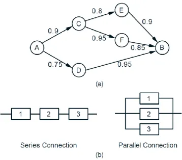
Example. Network connectivity. A computer network connects two nodes 𝐴 and 𝐵 through intermediate nodes 𝐶, 𝐷, 𝐸, 𝐹, as shown in Fig. 6, (a). For every pair of directly connected nodes, say 𝑖 and 𝑗, there is a given probability 𝑝𝑖𝑗 that the link from 𝑖 to 𝑗 is up. We
assume that link failures are independent of each other. What is the probability that there is a path connecting 𝐴 and 𝐵 in which all links are up?
Fig. 6: (a) Network for Example. The number next to each link (𝑖, 𝑗) indicates the probability that the link is up. (b) Series and parallel connections of three components in a reliability
problem.
subsystem consists in turn of several components that are connected either in series or in parallel; see Fig. 6, (b).
Let a subsystem consist of components 1, 2, … , 𝑚, and let 𝑝𝑖 be the probability that component 𝑖 is up (“succeeds”). Then, a series subsystem succeeds if all of its components are up, so its probability of success is the product of the probabilities of success of the corresponding components, i.e.,
𝑃(𝑠𝑒𝑟𝑖𝑒𝑠 𝑠𝑢𝑏𝑠𝑦𝑠𝑡𝑒𝑚 𝑠𝑢𝑐𝑐𝑒𝑒𝑑𝑠) = 𝑝1𝑝2⋯ 𝑝𝑚.
A parallel subsystem succeeds if any one of its components succeeds, so its probability of failure is the product of the probabilities of failure of the corresponding components, i.e.,
𝑃(𝑝𝑎𝑟𝑎𝑙𝑙𝑒𝑙 𝑠𝑢𝑏𝑠𝑦𝑠𝑡𝑒𝑚 𝑠𝑢𝑐𝑐𝑒𝑒𝑑𝑠) = 1 − 𝑃(𝑝𝑎𝑟𝑎𝑙𝑙𝑒𝑙 𝑠𝑢𝑏𝑠𝑦𝑠𝑡𝑒𝑚 𝑓𝑎𝑖𝑙𝑠) = 1 − (1 − 𝑝1)(1 − 𝑝2) ⋯ (1 − 𝑝𝑚).
Returning now to the network of Fig. 6, (a), we can calculate the probability of success (a path from 𝐴 to 𝐵 is available) sequentially, using the preceding formulas, and starting from the end. Let us use the notation 𝑋 → 𝑌 to denote the event that there is a (possibly indirect) connection from node 𝑋to node 𝑌. Then,
𝑃(𝐶 → 𝐵) = 1 − 1 − 𝑃(𝐶 → 𝐸 𝑎𝑛𝑑 𝐸 → 𝐵) 1 − 𝑃(𝐶 → 𝐹 𝑎𝑛𝑑 𝐹 → 𝐵) = 1 − (1 − 𝑝𝐶𝐸𝑝𝐸𝐵)(1 − 𝑝𝐶𝐹 𝑝𝐹𝐵) = 1 − (1 − 0.8 ∙ 0.9)(1 − 0.85 ∙ 0.95) = 0.946,
𝑃(𝐴 → 𝐶 𝑎𝑛𝑑 𝐶 → 𝐵) = 𝑃(𝐴 → 𝐶)𝑃(𝐶 → 𝐵) = 0.9 ∙ 0.946 = 0.851,
𝑃(𝐴 → 𝐷 𝑎𝑛𝑑 𝐷 → 𝐵) = 𝑃(𝐴 → 𝐷)𝑃(𝐷 → 𝐵) = 0.75 ∙ 0.95 = 0.712,
and finally we obtain the desired probability
𝑃(𝐴 → 𝐵) = 1 − 1 − 𝑃(𝐴 → 𝐶 𝑎𝑛𝑑 𝐶 → 𝐵) 1 − 𝑃(𝐴 → 𝐷 𝑎𝑛𝑑 𝐷 → 𝐵) = 1 − (1 − 0.851)(1 − 0.712) = 0.957.
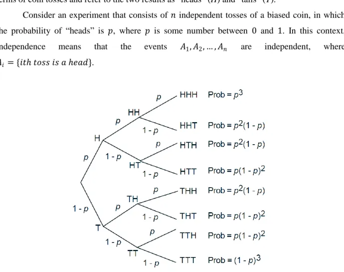
If an experiment involves a sequence of independent but identical stages, we say that we have a sequence of independent trials. In the special case where there are only two possible results at each stage, we say that we have a sequence of independent Bernoulli trials. The two possible results can be anything, e.g., “it rains” or “it doesn’t rain”, but we will often think in terms of coin tosses and refer to the two results as “heads” (H) and “tails” (T).
Consider an experiment that consists of 𝑛 independent tosses of a biased coin, in which the probability of “heads” is 𝑝, where 𝑝 is some number between 0 and 1. In this context, independence means that the events 𝐴1, 𝐴2, … , 𝐴𝑛 are independent, where
𝐴𝑖 = {𝑖𝑡ℎ 𝑡𝑜𝑠𝑠 𝑖𝑠 𝑎 ℎ𝑒𝑎𝑑}.
Fig. 7: Sequential description of the sample space of an experiment involving three independent
tosses of a biased coin. Along the branches of the tree, we record the corresponding conditional probabilities, and by the multiplication rule, the probability of obtaining a particular 3-toss sequence is calculated by multiplying the probabilities recorded along the corresponding path of
the tree.
obtain that the probability of any particular 𝑛-long sequence that contains 𝑘 heads and 𝑛 − 𝑘 tails is 𝑝𝑘(1 − 𝑝)𝑛−𝑘, for all 𝑘from 0 to 𝑛.
Let us now consider the probability
𝑝(𝑘) = 𝑃(𝑘 ℎ𝑒𝑎𝑑𝑠 𝑐𝑜𝑚𝑒 𝑢𝑝 𝑖𝑛 𝑎𝑛 𝑛 − 𝑡𝑜𝑠𝑠 𝑠𝑒𝑞𝑢𝑒𝑛𝑐𝑒),
which will play an important role later. We showed above that the probability of any given sequence that contains 𝑘heads is 𝑝𝑘(1 − 𝑝)𝑛−𝑘, so we have
𝑝(𝑘) = 𝑛𝑘 𝑝𝑘(1 − 𝑝)𝑛−𝑘,
where
𝑛
𝑘 = 𝑛𝑢𝑚𝑏𝑒𝑟 𝑜𝑓 𝑑𝑖𝑠𝑡𝑖𝑛𝑐𝑡 𝑛 − 𝑡𝑜𝑠𝑠 𝑠𝑒𝑞𝑢𝑒𝑛𝑐𝑒𝑠 𝑡ℎ𝑎𝑡 𝑐𝑜𝑛𝑡𝑎𝑖𝑛 𝑘 ℎ𝑒𝑎𝑑𝑠.
The numbers 𝑛𝑘 (called “𝑛choose 𝑘”) are known as the binomial coefficients, while the
probabilities 𝑝(𝑘) are known as the binomial probabilities. Using a counting argument one finds that
𝑛 𝑘 =
𝑛!
𝑘!(𝑛 − 𝑘)!, 𝑘 = 0, 1, … , 𝑛,
where for any positive integer 𝑖we have
𝑖! = 1 ∙ 2 ⋯ (𝑖 − 1) ∙ 𝑖,
and, by convention, 0! = 1. An alternative verification is sketched in the theoretical problems. Note that the binomial probabilities 𝑝(𝑘) must add to 1, thus showing the binomial formula
𝑛
𝑘 𝑝𝑘(1 − 𝑝)𝑛−𝑘 𝑛