Control-based imputation for sensitivity analyses in
informative censoring for recurrent event data
Fei Gao
1Guanghan F. Liu
2Donglin Zeng
1Lei Xu
2Bridget Lin
1Guoqing Diao
3Gregory Golm
2Joseph F. Heyse
2Joseph G. Ibrahim
11Department of Biostatistics, University of
North Carolina, Chapel Hill, NC, USA
2Merck Sharp & Dohme Corp., North
Wales, PA, USA
3Department of Statistics, George Mason
University, Fairfax, VA, USA
Correspondence
Fei Gao, Department of Biostatistics, University of North Carolina, Chapel Hill, NC, USA.
Email: [email protected]
In clinical trials, missing data commonly arise through nonadherence to the ran-domized treatment or to study procedure. For trials in which recurrent event endpoints are of interests, conventional analyses using the proportional inten-sity model or the count model assume that the data are missing at random, which cannot be tested using the observed data alone. Thus, sensitivity analy-ses are recommended. We implement the control-based multiple imputation as sensitivity analyses for the recurrent event data. We model the recurrent event using a piecewise exponential proportional intensity model with frailty and sam-ple the parameters from the posterior distribution. We impute the number of events after dropped out and correct the variance estimation using a bootstrap procedure. We apply the method to an application of sitagliptin study.
K E Y WO R D S
bootstrap, control-based imputation, missing data, multiple imputation, recurrent event data
1
I N T RO D U CT I O N
Recurrent event data are often collected in clinical trials. Examples include time to recurrent episodes of adverse experi-ences and reappearance of disease after remission. Although analyses typically focus on the time to first event, it is often of interest to take into account all recurrent events in the analysis.[1]Two categories of statistical models are available to
analyze recurrent event data. The first consists of modeling counts, and a common approach is the negative binomial (NB) model with or without zero inflation.[2]The second method models the recurrent time to event, and the most common
approach is the proportional intensity model either by gap time or total time.[3, 4, 5]The latter is often used for analysis
of recurrent episodes of adverse experiences in clinical trials because it provides estimates of the incidence rate for each treatment group in addition to the treatment comparison.
In clinical trials, nonadherence to the randomized treatment or to study procedure occurs in practice. Despite efforts to minimize missing data through careful planning and conduct, the amount of missing data could be nontrivial. When there are missing data, analysis using the proportional intensity model or count model based on the observed data implicitly assumes missing at random (MAR). This assumption cannot be tested or verified using the observed data. To assess the robustness and unbiasedness of the study findings against this assumption, sensitivity analyses are recommended by regulatory agencies.[6, 7]
proposed a general framework for control-based imputation for continuous (and noncensored) data. Two approaches that may be applied to recurrent event data are
• Copy reference: for the purpose of imputing the missing response data, a subject's whole distribution, both predeviation and postdeviation, is assumed to be the same as the reference group.
• Jump to reference: post deviation, the subject ceases randomized treatment, and subject's response distribution is now that of a “reference” group of subjects (while the response distribution prior to deviation follows that of randomized treatment).
For both of these approaches, an assumption is made that the missing data pattern is monotone (ie, every subject has complete data up to the point of a deviation, after which all data are missing), and postdeviation data in the reference arm are imputed under MAR.
For time to event analysis, control-based imputation assumes that the risk for censored subjects in the test drug group is higher (so more conservative) and similar to those in the control group. This assumption is reasonable and appealing to clinical scientists in superiority studies if no other medication is used after a subject in the test drug group discon-tinues from the test drug. This approach will also yield a conservative treatment effect estimate for safety endpoints if the test drug is expected to be superior to the control. Lu et al[9]considered a control-based imputation similar to the
jump to reference for time to event data with possibly informative censoring, in which the hazard for test drug subjects who discontinued is assumed to be between the hazard for test drug subjects who continued and the hazard for the sub-jects in the reference. Lipkovich et al[10]considered the tipping point approach where the event rate after discontinuation
for subjects in the treatment group is a certain percentage higher than a similar subject continued in the study. Para-metric (piecewise exponential baseline hazard), semi-paraPara-metric, and nonparaPara-metric imputation models were evaluated and compared.
For recurrent event data, Keene et al[11]specified a log-linear NB model with offset and samples the jump-to-reference
and copy-reference imputation parameters from the posterior distribution using a noninformative prior. Akacha and Ogundimu[12] considered copy-reference and tipping point control-based imputation for recurrent event data, where
the count after dropout is imputed from a posterior predictive distribution using asymptotic or bootstrap imputation to approximate the Bayesian data argumentation scheme. Both authors obtain variance estimators for the parameter estimates from control-based imputation using Rubin formula.[13]
It is well known that Rubin formula may overestimate the standard errors of the parameter estimates when dif-ferent models are used for imputation and/or analysis or when the imputation models are misspecified,[14] which
applies for control-based imputation. Lu[15] and Liu and Pang[16]considered the analysis of the longitudinal data and
examined the performance of Rubin formula in several simulation settings. They found that Rubin formula overes-timates the standard errors and that the inference may be over-conservative. Lu et al[9] encountered similar issues
in the analysis of time-to-event data and considered the use of the bootstrap approach to get appropriate standard errors.
In this paper, we implement control-based imputation in analyzing clinical trials with recurrent event data by sam-pling the parameters from the posterior distribution similar to that from Keene etal[11]However, we assume a piecewise
exponential proportional intensity model with frailty for the recurrent events. We correct the variance estimation through a bootstrap approach. Section 2 describes a motivating example in a diabetes clinical trial where a NB model is used to analyze the recurrent event data. The statistical methods for implementing control-based imputation are provided in Section 3. We examined the performance of proposed estimators and bootstrap method in Section 4. A detailed data analysis is presented in Section 5, followed by some discussion in Section 6.
2
M OT I VAT I N G E X A M P L E
Mathieu etal[17]described a randomized, double-blind, placebo-controlled parallel-group study to assess the efficacy and
hypoglycemia AEs during the 24-week double-blind treatment period. One of the study objectives was to demonstrate that sitagliptin reduces the incidence of hypoglycemia AEs.
A total of 658 subjects (329 in each group) were randomized and took at least one dose of study medication, of whom 295 (89.7%) in the sitagliptin group and 303 (92.1%) in the placebo group completed the 24-week follow-up in the study. Early study discontinuation was a common reason for missing data, and the reason for discontinuation may have been related to the event of interest, as explained below. Among the subjects who discontinued, the most common reason for discontinuation in both groups was AE (n=7 with sitagliptin vs n=6 with placebo). While these AEs may not be related to the outcome of interest (ie, hypoglycemia AEs), there were other reasons that may have been. For example, discontinuation due to hypoglycemia (repeated episodes despite progressive down-titration of insulin; n=1 with placebo) and hyperglycemia/lack-of-efficacy (n=3 with placebo) may have led to data censoring when hypoglycemia AEs were about to intensify or emerge had the subjects remained in the study. In addition, discontinuation reasons such as loss to follow-up (n=4 with sitagliptin vs n=3 with placebo) and physician decision (n=2 with sitagliptin vs n=5 with placebo) may imply dependent censoring for the analysis of hypoglycemia AEs. It is thus not possible to rule out missing not at random for such subjects, and it is not clear whether even a small amount of missing not at random data could have had an impact on the study findings.
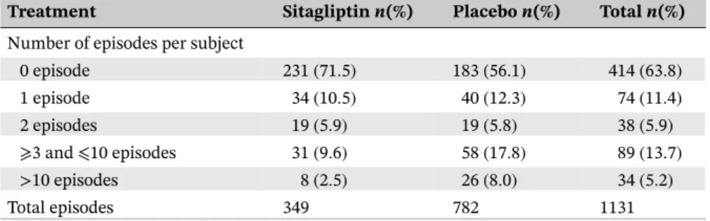
Nine subjects were excluded from the analysis due to missing baseline covariates, resulting in a total of 649 subjects who contributed to the analysis with 323 subjects in the sitagliptin group and 326 subjects in placebo group. On the basis of the observed data, 92 (28.5%) subjects in the sitagliptin group reported at least one hypoglycemia AE for a total of 349 hypoglycemia AEs, relative to 143 (43.9%) subjects in the placebo group for a total of 782 hypoglycemia AEs. Table 1 shows the distribution of the number of hypoglycemia AEs per subject by treatment group.
An NB regression model was used for the analysis of event rate of hypoglycemia AEs. The model included terms for treatment, baseline A1C value (a measure of glycemic control), baseline body weight, baseline daily insulin dose, and an offset for follow-up time (on the natural log scale). The model can be written as
log𝜇i=logCi+𝛼+𝛿Ai+𝛽TZi,
where𝜇iis the expected number of hypoglycemia AEs for subjecti;Ciis the follow-up time during the study for subject
i;Ziis the vector of baseline values for A1C, body weight, and daily insulin dose for subjecti;𝛼is the intercept;𝛿is the
treatment effect of sitagliptin on the rate of hypoglycemia AEs; and𝛽 ≡(𝛽A1C, 𝛽wt, 𝛽ins)is the effects of baseline values of
A1C, body weight, and daily insulin dose on the rate of hypoglycemia AEs.
The parameter estimates from the NB regression model are shown in Table 2. A significant reduction in event rate of hypoglycemia AEs was observed in the sitagliptin group compared to the placebo group. However, since this analysis
TABLE 1 Distribution of the number of episodes of hypoglycemia adverse events per subject
Treatment Sitagliptinn(%) Placebon(%) Totaln(%)
Number of episodes per subject
0 episode 231(71.5) 183(56.1) 414(63.8)
1 episode 34(10.5) 40(12.3) 74(11.4)
2 episodes 19(5.9) 19(5.8) 38(5.9) ⩾3 and⩽10 episodes 31(9.6) 58(17.8) 89(13.7) >10 episodes 8(2.5) 26(8.0) 34(5.2)
Total episodes 349 782 1131
TABLE 2 Parameter estimates from the negative binomial model
Parameter Estimate Std. Error Pvalue
Intercept −4.078 0.882 <.0001
Treatment −0.824 0.181 <.0001
Baseline A1C 0.064 0.090 .477
Baseline insulin 0.015 0.005 .002
assumed a constant event rate over time and that post-discontinuation data were MAR, sensitivity analyses with different missing data assumptions are needed to assess the impact of missing data on the findings from the NB regression.
3
STAT I ST I C A L M ET H O D O LO GY
In general, to conduct control-based imputation for recurrent hypoglycemia AEs, we first construct a recurrent events model. We then impute the number of recurrent events after dropout following the assumptions of different imputa-tion procedures. The sensitivity analysis for recurrent hypoglycemia AEs is then conducted based on the imputed data. We repeat the imputation and analysismtimes and use a bootstrap method for valid variance estimation. Details are provided below.
3.1
Recurrent events model with frailty
Consider a clinical study withnindependent subjects. We follow subjectiuntilCi ⩽ 𝜏i, where𝜏i denotes the time of
study end (eg, the last scheduled visit), and observemievents at times{t1i,…,tmi i}. DenoteAias the treatment andZias
the other covariates. We construct the model for recurrent eventsNi(t)based on subjects in a subset⊂{1,…,n}. For
subjecti∈, we assume thatNi(t)follows a proportional intensity model with gamma frailty, with
Λi(t;bi) = Λ(t)bieX
T
i𝛽,
whereXiis a vector of covariates considered in the recurrent events model, andbiisi.i.d.from Gamma distribution with
mean 1 and variance𝛾. If we choose= {1,…,n}, then we consider a recurrent events model for all the subjects in the study, and a natural choice ofXiis(Ai,Zi). If we choose = {i ∶i = 1,…,n,Ai = 0}, then the recurrent events
modeling is limited to the control group, andXishould not includeAi.
We assume that the baseline hazard functionΛ(t)is a piecewise exponential such that
𝜆(t) = K
∑
k=1
𝜆kI(sk−1<t⩽sk)
and
Λ(t) = K
∑
k=1
𝜆kI(t>sk−1) {min(t,sk) −sk−1},
where the parameters𝜆 = (𝜆1,…, 𝜆K)and the cutpoints are 0 = s0 < s1 < · · · < sK−1 < sK = ∞. The log-likelihood
function for(𝛽, 𝛾, 𝜆)is given by
ln(𝛽, 𝛾, 𝜆) =
∑
i∈
log
[
∫bi
∏
t⩽Ci
{
𝜆(t)bieX
T
i𝛽
}ΔNi(t)
exp
{
−Λ(Ci)bieX
T
i𝛽
}(1∕𝛾)1∕𝛾
Γ(1∕𝛾)b
1∕𝛾−1
i exp
(
−bi 𝛾
)
dbi
]
=∑
i∈
[
logΓ
{
1
𝛾 +Ni(Ci)
}
−logΓ
( 1 𝛾 ) +∫ Ci 0 {
log𝛾+log𝜆(t) +XiT𝛽}dNi(t)
−
{
1
𝛾 +Ni(Ci)
}
log
{
1+𝛾Λ(Ci)eX
T
i𝛽
}]
.
(1)
The posterior distribution ofbigiven the data and the parameters(𝛽, 𝜆, 𝛾)is proportional to
∏
t⩽Ci
{
𝜆(t)bieX
T
i𝛽
}ΔNi(t)
exp
{
−Λ(Ci)bieX
T
i𝛽
}(1∕𝛾)1∕𝛾 Γ(1∕𝛾) b
1∕𝛾−1
i exp
(
−bi 𝛾
)
∝b1∕𝛾+Ni(Ci)−1
i exp
[
−bi
{
1
𝛾 + Λ(Ci)eX
T
i𝛽
}]
.
Therefore, the posterior distribution ofbiis Gamma distribution with shape parameter 1∕𝛾+Ni(Ci)and rate parameter
1∕𝛾+ Λ(Ci)eX
T
3.2
Imputation model
For subjects who dropped out before the last scheduled visit, ie,Ci< 𝜏i, we treat the subsequent recurrent eventsÑi(t)as
missing data and impute the number of events after dropout from an imputation model with intensity
̃
Λi(t;bi) = Λ(t)bieX̃
T
i𝛽.
Here,X̃iis the value of the covariates used for imputation.
Given this intensity function, the process after dropoutÑi(t)follows a nonhomogeneous Poisson process. The total
number of events in(Ci, 𝜏i]givenbiis then Poisson distributed with rate
{
̃
Λi(𝜏i;bi) −Λ̃i(Ci;bi)
}
. We integrate outbiand
obtain
Pr{Ni(𝜏i) −Ni(Ci) =x} =Ebi
⎡ ⎢ ⎢ ⎢ ⎣ {
̃
Λi(𝜏;bi) −Λ̃i(Ci;bi)
}x
x! exp
{
−Λ̃i(𝜏;bi) +Λ̃i(Ci;bi)}⎤⎥⎥
⎥ ⎦
= Γ{x+1∕𝛾+Ni(Ci)}
x!Γ{1∕𝛾+Ni(Ci)}
[
𝛾{Λ(𝜏i) − Λ(Ci)}eX̃
T
i𝛽
]x{
1+𝛾Λ(Ci)eX
T
i𝛽
}1∕𝛾+Ni(Ci)
×
[
1+𝛾{Λ(𝜏i) − Λ(Ci)}eX̃
T
i𝛽+𝛾Λ(Ci)eXiT𝛽
]−{x+1∕𝛾+Ni(Ci)} .
The number of events after dropout is then distributed as NB with number of successesk =1∕𝛾 +Ni(Ci)and success
probability
p= 1+𝛾Λ(Ci)e XT
i𝛽
1+𝛾{Λ(𝜏i) − Λ(Ci)}eX̃
T
i𝛽+𝛾Λ(Ci)eXiT𝛽 .
3.3
Different imputation procedure
We consider 2 types of control-based multiple imputation approaches to perform the sensitivity analysis: copy reference and jump to reference.
In copy reference control-based imputation, we assume that the whole distribution for the treated subject, both before and after dropout, is the same as the control group. Therefore, we first model recurrent events for subjects in the control group, ie,= {i∶i=1,…,n,Ai= 0},Xi=Zi. Then, we impute the number of events after dropout withX̃i =Zifor
both groups.
In jump to reference control-based imputation, we assume that after a subject drops out, the response distribution is that of a subject in the control group. Therefore, we model recurrent events for all the subjects, ie, = {1,…,n}, Xi= (Ai,Zi). Then, we impute the number of events after dropout withX̃i= (0,Zi)for both groups.
For copy reference and jump to reference procedures, we make different assumptions on the distribution of recurrent event before dropout for subjects in the treatment group. Therefore, the posterior distributions ofbigiven events before
dropout are very different under the two assumptions, such that the imputation models are quite different. If there is no frailty, then the imputation models will be very similar since the distribution of events after dropout is independent of before dropout distribution given baseline covariates.
To compare with control-based imputation, we also implemented imputation under MAR. For imputation under MAR, we model recurrent events with= {1,…,n},Xi= (Ai,Zi)and impute withX̃i= (Ai,Zi)for both groups.
3.4
Inference using the bootstrap
The bootstrap procedure for control-based imputation for recurrent event data is as follows:
Step 1. We first fit the recurrent events frailty model corresponding to the imputation assumptions and drawmsamples of the parameters(𝛽(j), 𝛾(j), 𝜆(j))(j = 1,…,m)from the posterior distribution based on model 1 using
noninforma-tive priors for the parameters. The samples are obtained using proc MCMC in SAS, and the SAS code is given in the Appendix of the paper.
Step 2. For imputationj=1,…,m, impute the number of events after dropout using the parameters(𝛽(j), 𝛾(j), 𝜆(j))and
the imputation assumptions. Perform the primary analysis based on the imputed values, and obtain the estimateŝ𝜃(j).
Step 4. For each bootstrap sampleb=1,…,B, perform steps 1 and 2 to obtain the estimateŝ𝜃b(j)(j=1,…,m). The overall point estimate is then ̂𝜃 ≡ ∑mj=1̂𝜃(j)∕m. The variance for ̂𝜃is estimated by the sample variance of the
estimateŝ𝜃b≡∑mj=1̂𝜃
(j)
b ∕m,b=1,…,B, from theBbootstrap samples.
4
S I M U L AT I O N ST U D I E S
We performed simulation studies to evaluate the performance of the proposed methods. We considered a study population with 100 subjects in the treatment arm and 100 subjects in the control arm. We considered one baseline covariateZ ∼
Unif(0,1). We denote the intensity functions
ΛC(t;b) =0.5tbe0.5Z
and
ΛT(t;b) =0.5tbe−0.8+0.5Z,
wherebis fromGamma(1,1). For each subject, we simulated a noninformative dropout timeC=B𝜏+ (1−B)Unif(0, 𝜏), whereBis an independent binary random variable with mean 0.8 and𝜏 = 5 is the fixed follow-up time for the study. Therefore, the dropout rates for both arms are 20%.
For each subject, we first generated the random effectbindependently. The recurrent events for subjects in the control arm were generated with intensity functionΛC(t;b). The recurrent events for subjects in the treatment arm who complete
the study were generated with intensity functionΛT(t;b). For subjects in the treatment arm who fail to complete the study,
we considered 3 approaches to generate the recurrent events, reflecting different assumptions of jump to reference, copy reference, and MAR.
1. Copy reference. We generated the recurrent events with intensity functionΛC(t;b)throughout the study.
2. Jump to reference. We generated the recurrent events with intensity functionΛT(t;b)before dropoutCandΛC(t;b)
afterC.
3. MAR. We generated the recurrent events with intensity functionΛT(t;b)throughout the study.
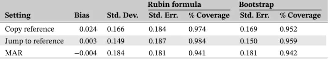
Table 3 summarizes the simulation results of treatment effects based on 1000 replicates. We calculated the true values using the average of the parameter estimates from the full generated datasets with events observed after dropout. The true values for the treatment effect under the three settings are−0.573,−0.690, and−0.796. The parameter estimators for the treatment effects are virtually unbiased. Rubin formula tends to overestimate the true variabilities for treatment effect in the copy reference and jump to reference settings. The coverage probabilities for the 95% confidence intervals are larger than the nominal levels, especially in the jump to reference setting. The bootstrap method gives accurate estimates of true variabilities and proper coverages for the treatment effect.
5
DATA A NA LY S I S
We applied the sensitivity analysis methods to the recurrent hypoglycemia events in the diabetes trial as described in Section 2. We usedm=50 imputations,K=8 cutpoints, and selecteds1,…,sKto have approximately equal numbers of
events in each interval. To ensure reasonably small autocorrelations in the MCMC samples, we standardized the baseline covariates except for treatment, and set the burn-in=5000 and thinning=100. Table 4 shows the posterior estimates of the parameters from the recurrent events frailty model. Treatment had a significant effect on the intensity of recurrence of hypoglycemia AEs.
TABLE 3 Summary statistics for treatment effect in the simulation studies
Rubin formula Bootstrap
Setting Bias Std. Dev. Std. Err. % Coverage Std. Err. % Coverage
Copy reference 0.024 0.166 0.184 0.974 0.169 0.952 Jump to reference 0.003 0.149 0.187 0.984 0.150 0.959
MAR −0.004 0.184 0.181 0.941 0.181 0.942
TABLE 4 Summary of posterior estimates for the parameters in the recurrent events models
Model Placebo group Both groups
parameter Mean Std. Dev. Mean Std. Dev.
Treatment −0.784 0.163
Baseline A1C 0.132 0.131 0.077 0.104 Baseline insulin 0.223 0.134 0.345 0.091 Baseline weight −0.256 0.140 −0.273 0.098
𝜆1 0.007 0.001 0.008 0.001
𝜆2 0.014 0.002 0.014 0.002
𝜆3 0.017 0.003 0.017 0.003
𝜆4 0.016 0.002 0.019 0.003
𝜆5 0.020 0.003 0.017 0.002
𝜆6 0.021 0.003 0.019 0.003
𝜆7 0.022 0.003 0.020 0.003
𝜆8 0.021 0.004 0.020 0.003
Frailty variance (𝛾) 3.905 0.551 4.529 0.390
TABLE 5 Parameter estimates from multiple imputation with bootstrap (proposed method)
Multiple Control-based
imputation Copy reference Jump to reference MAR
Parameter Estimate Std. Err. Pvalue Estimate Std. Err. Pvalue Estimate Std. Err. Pvalue
Intercept −4.155 1.056 <.0001 −4.099 1.068 <.0001 −4.089 1.096 <.0001 Treatment −0.784 0.183 <.0001 −0.755 0.168 <.0001 −0.815 0.198 <.0001
Baseline A1C 0.071 0.103 .489 0.068 0.104 .513 0.067 0.106 .530
Baseline insulin 0.015 0.004 .0002 0.015 0.004 .0001 0.015 0.004 .0002 Baseline weight −0.014 0.006 .014 −0.015 0.006 .011 −0.015 0.006 .013 Dispersion parameter 4.261 0.379 <.0001 4.308 0.378 <.0001 4.308 0.379 <.0001
Abbreviation: MAR, missing at random.
TABLE 6 Parameter estimates from multiple imputation based on Keene et al[11]method
Multiple Control-based
imputation Copy reference Jump to reference MAR
Parameter Estimate Std. Err. Pvalue Estimate Std. Err. Pvalue Estimate Std. Err. Pvalue
Intercept −4.087 0.885 <.0001 −4.085 0.895 <.0001 −4.073 0.884 <.0001 Treatment −0.812 0.182 <.0001 −0.776 0.183 <.0001 −0.824 0.181 <.0001
Baseline A1C 0.065 0.091 .476 0.062 0.092 .499 0.064 0.090 .482
Baseline Insulin 0.015 0.005 .001 0.015 0.005 .001 0.015 0.005 .001
Baseline Weight −0.015 0.006 .009 −0.014 0.005 .002 −0.015 0.006 .008 Dispersion Parameter 4.371 0.403 <.0001 4.339 0.401 <.0001 4.362 0.403 <.0001
Abbreviation: MAR, missing at random.
We also implemented the method proposed by Keene et al,[11]where a NB model with an offset is assumed for the
recurrent events and the standard errors are estimated based on Rubin formula. Note that the point estimate from Keene method is equivalent to that of our method with an exponential baseline intensity function, ie, the number of cutpoints K=1. Table 6 shows the parameter estimates using Keene method with 1000 multiple imputations. The point estimates for the treatment effect for the two control-based methods are similar to that of our method. The standard errors using Rubin formula are similar for the three imputation methods.
6
D I S C U S S I O N A N D CO N C LU S I O N S
In the analysis of time to event data, noninformative or independent censoring is commonly assumed. This assumption is analogous to the MAR assumption in the analysis of longitudinal data. It is well known that this assumption may not be verifiable from the observed data. Sensitivity analyses are therefore recommended to check the robustness of the analysis against this censoring or missing data assumption. In this paper, we investigated how to implement control-based imputation for proportional intensity frailty models for conducting sensitivity analyses for clinical trials with recurrent events.
Control-based imputation has become attractive to clinical trial scientists for its explicit specification of the imputation model for the missing data. It assumes that the distribution of the missing data after dropout for subjects in the test drug group is similar to that in the control group. This is appealing because it provides a conservative estimate for the treatment effect compared to the estimate obtained under noninformative censoring. For trials with recurrent events, we considered a flexible proportional intensity model with a piecewise exponential baseline hazard function. The number of intervals for the piecewise baseline hazard can be determined by choosing an equal number of events within each interval. A similar approach has also been considered for sensitivity analyses for time to event data,[15]where the authors used simulations
to show that the results from a piecewise exponential baseline hazard is generally similar to that from a nonparametric baseline hazard function.
A gamma frailty was considered in the proportional intensity model to account for intrasubject correlation for recur-rent events. To implement control-based imputation models, we derived the marginal cumulative intensity function after integrating out the frailty parameter and showed that the number of events after dropout up to the end of study follows a NB distribution. This property was used to conduct control-based imputation including the copy-reference and jump-to-reference methods. The bootstrap was used to obtain appropriate standard errors for testing the treat-ment effect after control-based multiple imputation because Rubin formula tends to over-estimate the standard errors.
As noted in the application of the proposed approach to the sitagliptin trial, control-based imputation may produce a conservative point estimate for the treatment difference; that is, it is attenuated towards zero. However, the power for testing the treatment difference when the bootstrap is used to get the variance may not be necessarily lower than that of a likelihood-based analysis. This is because the estimands of the true parameters to be tested of these two approaches are different. In the NB model with non-informative censoring, the estimand is equivalent to the treatment difference if all subjects were followed to the given duration. Control-based imputation addresses a different estimand, which assumes that the intensity function of the test drug is similar to that of the control group. Similar phenomena and results have been observed in the analysis of repeated measures for longitudinal data.[16]
The proposed imputation models assume piecewise exponential cumulative hazard function and proportional intensity for recurrent events given baseline covariates and frailty. Those model assumptions may also suffer from potential model misspecification. We can relax the assumptions for the imputation models, such as allowing nonproportional intensity or estimating the baseline cumulative hazard functions nonparametrically. The extended method may be computationally more intensive.
The proposed methods only handle the missing responses due to early dropout but not for missing covariates. In the analysis of real data example, a few patients with missing covariates were excluded. Some future research is required to deal with both missing responses from dropout and missing covariates.
O RC I D
Fei Gao http://orcid.org/0000-0001-6797-5468
R E F E R E N C E S
[1] R. J. Cook, J. Lawless,The Statistical Analysis of Recurrent Events, Springer, New York2007. [2] R. Berk, J. M. MacDonald,J. Quantitative Crim.2008,24, 269.
[3] R. L. Prentice, B. J. Williams, A. V. Peterson,Biometrika1981,68, 373. [4] P. K. Andersen, R. D. Gill,The Ann. Stat.1982,10, 1100.
[5] L. J. Wei, D. Y. Lin, L. Weissfeld,J. Am. Stat. Assoc.1989,84, 1065.
[6] National Academy of Sciences,The Prevention and Treatment of Missing Data in Clinical Trials. Panel on Handling Missing Data in Clinical Trials. Committee on National Statistics, Division of Behavioral and Social Sciences and Education, The National Academies Press, Washington, DC2010.
[7] European Medicines Agency, Guideline on Missing Data in Confirmatory Clinical Trials, Available from: http://www.ema.europa.eu/ docs/en_GB/document_library/Scientific_guideline/2010/09/WC500096793.pdf,2010. (accessed: August 4, 2017)
[8] J. R. Carpenter, J. H. Roger, M. G. Kenward,J. Biopharm. Stat.2013,23, 1352. [9] K. Lu, D. Li, G. G. Koch,Stat. Biopharm. Res.2015,7, 199.
[10] I. Lipkovich, B. Ratitch, M. O'Kelly,Pharm. Stat.2016,15, 216.
[11] O. N. Keene, J. H. Roger, B. F. Hartley, M. G. Kenward,Pharm. Stat.2014, 13, 258. [12] M. Akacha, E. O. Ogundimu,Pharm. Stat.2016,15, 4.
[13] D. B. Rubin,Multiple Imputation for Nonresponse in Surveys, Wiley, New York1987. [14] J. M. Robins, N. Wang,Biometrika2000,87, 113.
[15] K. Lu,Stat. Med.2014,33, 1134.
[16] G. F. Liu, L. Pang,J. Biopharm. Stat.2016.5, 92.
[17] C. Methieu, R. R. Shankar, D. Lorber, G. Umpierrez, F. Wu, L. Xu, G. T. Golm, M. Latham, K. D. Kaufman, S. S. Engel,Diabetes Ther. 2015,6, 127.
How to cite this article: Gao F, Liu GF, Zeng D, et al. Control-based imputation for sensitivity
analyses in informative censoring for recurrent event data. Pharmaceutical Statistics. 2017;16:424–432.
![TABLE 6 Parameter estimates from multiple imputation based on Keene et al [ 11 ] method Multiple Control-based](https://thumb-us.123doks.com/thumbv2/123dok_us/8215265.2178035/7.892.97.797.694.874/table-parameter-estimates-multiple-imputation-keene-multiple-control.webp)
