To appear in Proc. 11th ACM-SIAM Symp. on Discrete Algorithms, San Francisco, CA c SIAM 2000.
Engineering the Compression of Massive Tables: An Experimental Approach
Adam L. Buchsbaum
Donald F. Caldwell
Kenneth W. Church
Glenn S. Fowler
S. Muthukrishnan
Abstract
We study the problem of compressing massive tables. We devise a novel compression paradigm—training for lossless compression— which assumes that the data exhibit dependencies that can be learned by examining a small amount of training material. We develop an experimental methodology to test the approach. Our result is a system, pzip, which outperformsgzipby factors of two in compression size and both compression and uncompression time for various tabular data.Pzipis now in production use in an AT&T network traffic data warehouse.
1 Introduction
We study the problem of compressing massive tables, which arises naturally in corporate data warehouses. Our goal is to provide a working system that can be put into pro-duction use and achieve 100:1 compression, in particular, one that can compress 10s of TB of data into 100s of GB. We devise a novel compression strategy—training for loss-less compression—which can leverage standard compression methods, and we demonstrate its effectiveness experimen-tally. In the process, we identify the requirements for our compression application and design algorithmic solutions to various technical problems. The system we built,pzip, can compress 1 TB of data from AT&T’s network traffic data warehouse into about 28 GB, small enough to fit on one PC disk and a two-fold improvement over existing solutions (in time as well as space).Pzipis now in production use in the warehouse.
Our motivating applications are tables of traffic data from telecommunication networks. For example, the AT&T voice communications network generates a record of each phone call it carries. A typical record consists of several hundred bytes and depicts network-level information (e.g., endpoint exchanges), time-stamp information (e.g., start and end times), and billing-level information (e.g., applied tariffs). This application generates about 1 TB of data per month and is just one example of the many different tables that AT&T and other corporations generate. Others include switch- and router-level traffic data, equipment sensor data (e.g., alarm status), and credit card transaction records. These data have certain unifying characteristics: they have
AT&T Labs, Shannon Laboratory, 180 Park Ave., Florham Park, NJ 07932;falb,dfwc,kwc,gsf,[email protected].
fixed-length records and fields, they are written once but read many times, and they are truly massive (TBs per year). Furthermore, they typically contain much redundancy.
On the other hand, they are not text corpora (English, DNA, etc.), multimedia (images, audio, etc.), or WWW data (catalogs, bibliographies, XML files, etc.) Developing se-mantic compression techniques for each of these is an inde-pendent research area. Such methods can exploit domain-specific information, which is problematic in our setting for reasons explained below. Furthermore, our data sets are larger than most commercial data sets. Most dictionaries, corpora, etc., also are not this large. (For example, The Ox-ford English Dictionary consumes less than 10 GB; the As-sociated Press Newswire generates about one million words of text per week.)
Traditionally, compression is desirable because it saves not only storage space but also the I/O bandwidth (to disks, tapes, etc.) for accessing data. An added benefit is the sav-ings in network bandwidth for transmitting data. This inter-ests AT&T, where traffic tables may be shipped repeatedly to many centers: for fraud detection, billing, report generation, auditing, marketing, archival, customer care, and data analy-sis in general. The benefit of compression is thus saving not only storage space for a single copy of the data, with propor-tional effects on capital requirements for data warehouses, but also the cumulative cost of storing and transporting mul-tiple copies of the data over the system for its entire lifespan, which may well be several years.
and maintained. Finally, it is preferable that any solution be general, applying to the many different tables, or portions of tables, that are processed. Thus we cannot exploit domain-specific syntactic or semantic information.
Studying massive tables is a new focus in compression research. To distinguish our context from extant ones, con-sider the related field of database compression, where rela-tional data may be viewed as tables. This differs from our table compression problem in many ways. First, the goals are different. Database compression stresses the preserva-tion of indexing—the ability to retrieve an arbitrary record— under compression [7]. Table compression does not re-quire indexing to be preserved. Next, the data are different. Database records are often dynamic, unlike table data, which have a write-once discipline. Databases consist of hetero-geneous data, possibly with several string fields of variable length; table data are more homogeneous, with fixed field lengths. Also, non-tabular databases are not routinely TBs in size. (An exception is NASA’s EOSDIS database [13], which anticipates processing 1 TB of satellite images every two weeks.) Finally, the approaches to database compression include lightweight techniques such as compressing each tu-ple by simtu-ple encodings [7, 8] and tiling the entire table [8]. These approaches are not appropriate for table compression: the former is too wasteful, and the latter too expensive and cumbersome.
Our contribution is a novel approach for the table com-pression problem: lossless comcom-pression via training. The idea is to construct a compression plan for the table by study-ing a very small trainstudy-ing set off line. To do so, we assume that the data can be modeled by an underlying source that can be learned from a small sample. We further assume and exploit dependencies in the columns of the data in one of two ways: (1) implicitly, by grouping the columns that compress well together; and (2) explicitly, by determining a depen-dency tree among the columns. We then employ the com-pression plan on the entire dataset. To test our assumptions, we implement algorithms to construct compression plans on some training sets, and we compress test sets with respect to the plans. We compare the resulting compression to the straightforward approach of treating the tables as text and applying Lempel-Ziv compression [20, 21]. It will be clear that comparable performance would falsify our assumptions about the data dependencies. In all cases, however, our algorithms provide substantial compression improvements. While training has been applied to lossy compression, e.g., in speech coding [12, 15], ours is the first known instance of applying training to lossless compression.
For our primary application, compression exploiting implicit dependencies outperformed that using explicit de-pendencies. We have implemented the corresponding algorithm—optimum partitioning—inpzip, a fully work-ing software system for compresswork-ing table data, which has
been deployed in the AT&T network traffic data warehouse. Pzipachieves factors of about 2 improvement in compres-sion size and both comprescompres-sion and uncomprescompres-sion time over gzip, the method previously used in this application.
In Section 2, we discuss the table compression problem further and define our assumptions regarding data dependen-cies. In Section 3, we present technical problems that ex-ploit our assumptions, and we give algorithmic solutions to these problems. In Section 4, we present our experimental results, and in Section 5, we discuss thepzipsystem and some additional applications. In Section 6, we summarize our contributions and present directions for future work.
2 Problem Discussion
Our input consists of a table, T, of a large number of rows, each of length n bytes. We define column i to be the projection of the ith byte of each row, for 1
i n. (A byte is the smallest unit of data that can be easily and rapidly accessed; moreover, this level of granularity captures patterns among larger lexical units.) The table compression problem is to compressT, such that the requirements discussed in Section 1 are satisfied.
From an information-theoretic point of view,T can be treated as a string, e.g., of bytes in row-major order. It would thus suffice to perform Lempel-Ziv [20, 21] or Huffman [9] compression, yielding provably optimal asymptotic perfor-mance in terms of certain ergodic properties of the source that generates the table. This does not, however, adequately solve the table compression problem. For specific classes of inputs, e.g., tables of network traffic data, the optimality re-sults may not necessarily hold. In particular, the optimality results hold only with respect to compression methods that likewise treatT as a (byte) string; i.e., methods that do not account for complex dependencies inT. Some compression does result, however, and we use this method as our bench-mark in Section 4.
We need a few technical definitions. Denote byT[i℄the
ith column ofT. Denote byT[i;j℄the interval of columns ithroughj ofT. Finally, denote byS(C)the size of the result of compressing some intervalC of columns, in row-major order, using an arbitrary but fixed compressor.
2.1 Assumptions. Our approach to the table compression
problem assumes that there are dependencies among the columns ofT. In particular, we will consider dependencies of two types: combinational and differential.
DEFINITION2.1. Two contiguous intervals of columns
T[i;j℄andT[j+1;`℄are combinationally dependent if
S(T[i;j℄)+S(T[j+1;`℄)>S(T[i;`℄):
columns are dependent, without determining which columns are dependent on the others.
DEFINITION2.2. Column T[j℄ is differentially dependent
on columnT[i℄if
S(T[j℄)>S(T[i℄ T[j℄);
whereT[i℄ T[j℄is the column formed by taking the
row-wise difference between columnsT[j℄andT[i℄.
Differential dependency is an explicit dependency be-tween columns, in that it determines which column is de-pendent on the other. In general, we might compressT[j℄ andT[i℄ T[j℄by different methods, and we might consider other transformationsT[i℄T[j℄. This does not affect the ensuing discussion.
Our approach also makes the important assumption that the data is generated by some source that is well behaved, in particular, that dependencies (such as those above) among columns, if they exist, can be captured by examining a small amount of data, independent of the size ofT.
3 Algorithmic Issues
We design compression schemes based on the assumptions embodied in Definitions 2.1 and 2.2.
3.1 Combinational Approach. We can exploit
combina-tional dependencies as follows. Consider a partition,P, ofT into intervalsT[p
0 + 1;p
1 ℄;T[p
1 + 1;p
2
℄;:::;T[p ` 1
+ 1;p `
℄, such that p
0
= 0 and p `
= n. We refer to an interval T[p
i 1 +1;p
i
℄in P as a class. We define the cost of P to be
S(P)= ` X
i=1 S(T[p
i 1 +1;p
i ℄):
The goal is find an optimum partition, i.e., ^
P such that S(
^
P)=min P
S(P).
We can find an optimum partition as follows. Define
E(i) to be the cost of an optimum partition of T[1;i℄ for i1, and defineE(0)=0. Then fori1,
E(i)= min 0ji 1
E(j)+S(T[j+1;i℄):
Assuming that the cost S(T[j;i℄) has been computed for all 1 j i n, we can compute E(n) (and the corresponding partition) in O(n
2
)time by simple dynamic programming.
We call this optimum partitioning. This gives the following compression plan for compressingT: compress each class in the optimum partition independently in row-major order.
We can further speed up the dynamic programming, under the assumption that there are many optimum or near
optimum partitions for compressingT, and that among these are some in which the classes are not too wide. To do so, we develop a “chunking” approach, in which, for some
1 k <n, we divide thencolumns intodn=ke pairwise-disjoint intervals of size at mostkeach, and solve our general problem on each such interval. The running time becomes
O(nk). We call this chunk partitioning, and it likewise returns a compression plan.
3.2 Differential Approach. We can exploit differential
dependencies as follows. Consider a partition of the n columns of T into two sets, P and
P = [1;n℄nP. We treat the columns inP as source columns and those in
P as
derived columns. Given a mapping :
P ! P, we define the cost,S(P;)to be
X
p2P
S(T[p℄)+ X
p2
P
S(T[(p)℄ T[p℄):
The goal is to find a pair(P;)of minimum cost.
This is precisely the facility location problem [17]. We will assume that the differential cost is a metric. In general, this depends on the base compressor. We apply the simple, greedy algorithm for this problem [14].
At any time, we have a candidate pair ( ^
P;^). We determine the smallest cost solution,(
^ P 0
;^ 0
), obtained by 1. removing a column from ^
P, 2. adding a column to ^
P, or
3. substituting one of the columns in ^
Pfor one not in ^ P. (Ties are broken arbitrarily.) If S(
^ P 0
;^ 0
) < S( ^
P;)^ , then we set ^
P ^ P 0
and^ ^ 0
and iterate. Otherwise we are done. We call this greedy differential compression. The final solution is roughly5-optimal under the metric assumption [14]. Better approximations [3, 4, 5, 11] are known, but the greedy algorithm suffices for our purpose of testing the presence of differential dependencies.
Greedy differential compression produces the follow-ing compression plan: compress each column in ^
P indepen-dently, and for each columnp62
^
P, compressT[^(p)℄ T[p℄.
3.3 Lossless Compression via Training. Our overall
ap-proach is thus the following.
1. Select a small subsetT 0
Tas training material. 2. Using T
0
, compute a compression plan, P, forT by either the combinational or differential approach.
3. CompressTwith the compression planP.
generated a compression plan, we can use it to compress future tables generated by the same source as T. Training is thus an off-line procedure.
So far, we have abstracted the base problem of comput-ing S(T[i℄) andS(T[i;j℄). Rather than develop our own base compression method, we decided to use one of the stan-dard programs, which have already been well optimized: e.g., compress[18, 21], gzip [20], andvdelta [10]. Each is fast, on-line, and well-suited to our application. Of other available compressors, we note thatPPM[6, 19], which exploits context sensitivity and thus seems applicable to ta-ble data, and bzip [1] are too slow for our environment, although attempts have been made to tunePPMfor speed at the expense of compression size [16]. We therefore do not usebzipandPPMin our compression scheme, but we do compare our scheme againstbzipandPPMby themselves. We note but do not consider in this paper hybrid approaches, in which we pick the best compressor for a given interval. We can even nest the differential approach within the combi-national approach.
4 Experiments
4.1 Methodology. We summarize our assumptions as
fol-lows.
1. Our data sets present combinational dependencies.
2. The combinational approach is likely to induce some (near) optimum partition in which no class is wide.
3. Our data sets present differential dependencies.
4. The above dependencies can be detected with a small amount of training data, independent of the size ofT.
We fix gzip as our underlying compression method. While this does not explore the range of possible base com-pressor options, it suffices to test our approach. As bench-mark R, we apply gzip to T in row-major order, corre-sponding to the usage ofgzipwithout off-line training; as benchmark C, we applygziptoT in column-major order, corresponding to the other extremal partition in which no combinational or differential dependencies exist. We thus designed experiments to compare the performance of
1. optimum partitioning to the benchmarks,
2. chunk partitioning to optimum partitioning, and
3. the greedy differential compression to both optimum partitioning and benchmark C.
Each experiment has the potential to falsify one of our assumptions. If either benchmark outperforms optimum par-titioning (with respect to output size), then our data sets do not present combinational dependencies. If optimum parti-tioning significantly outperforms chunk partiparti-tioning, then all
(near) optimum partitions must have at least one wide class. If benchmark C outperforms the greedy differential compres-sion, then our data sets do not present differential dependen-cies. We discuss testing assumption (4) below.
For each experiment, we produced a compression plan by running the corresponding algorithm on a training data set. Using the resulting plan, we compressed a disjoint test data set, and we compared the compression performance (time and size) to that of the benchmark(s) for that goal. Although size of compressed output is the metric by which our assumptions can be falsified, we also measured running times, to assess the practicality of our methods. This method-ology extends to assess other, similar compression systems.
We also varied the amount of training data available, to gauge the effect of training size on compression perfor-mance. This is only the first step in testing assumption (4). If we do not see compression performance stabilize at some point as we increase the amount of training data, then as-sumption (4) is likely falsified. After observing this stabi-lization, however, a second test will be required: namely, to fix the training set size above the point at which we ob-served stability and increase the test set size arbitrarily. If the relative performance of the compression systems being compared does not remain stable, again assumption (4) is likely falsified. Otherwise, we will have evidence supporting assumption (4). Although this second experiment remains to be conducted, based on our results we do not expect assump-tion (4) to be falsified.
Finally, we compared the best results from the above experiments with isolated usages of compressors based on the Burrows-Wheeler transform [1] and prediction by par-tial match (PPM) [6, 19]. The goal was to assess empir-ically the benefit of our training scheme, which leverages standard compression technology, versus other methods that claim improved compression via sophisticated analyses of the source data.
Data. We used 100,000 records from a network traffic
data warehouse. Each record is 781 bytes and pertains to an individual network event. The warehouse receives approximately one billion records per month, so effective compression is critical to this application. From the 781 columns of bytes, we extracted the 90 with the highest frequency: i.e., the number of times the value of the byte changed as the column was scanned top-down. We explain this in Section 5; basically, in our real application, the other 691 columns were compressed more effectively using incomparable methods.
way left the corresponding rest of the data as the test set. In all our experiments, we used the training sets to generate the corresponding compression plans, and we conducted the compression experiments using those plans and the test sets.
Software. To run the experiments, we implemented the
following tools.
pin. Given a training set, pin computes a compression plan based on optimum partitioning.
pzip. Given a compression plan computed bypin,pzip compresses a test set with respect to the plan. It encodes enough of the plan into the output (which is included in the output size results reported) so that, given a com-pressed file,pzipwill uncompress it without needing the original plan. (Pin andpzip actually form our working system, and we discuss them in greater detail in Section 5.)
colsel. Given a training set, colselcomputes a com-pression plan based on the greedy differential algo-rithm.
cszip. Given a compression plan computed bycolsel,
cszipcompresses a test set with respect to the plan.
It encodes enough of the plan into the output (which is included in the output size results reported) so that, given a compressed file, cszip will uncompress it without needing the original plan.
Pzipandcszipuse thezliblibrary, version 1.1.3,1
to compress the intervals and columns, respectively.
System. All the training and experiments were run on
one 250 MHz MIPS R10000 processor on a 16-processor SGI Origin 2000 running IRIX 6.5, with 10 GB of main memory. Each time reported is the median of five runs, summing user and system time for each run.
4.2 Experiments and Results.
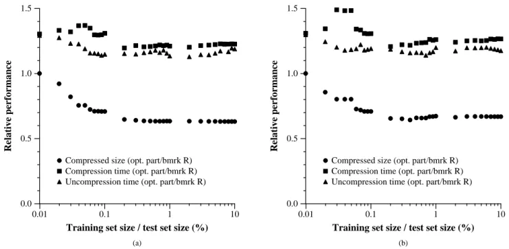
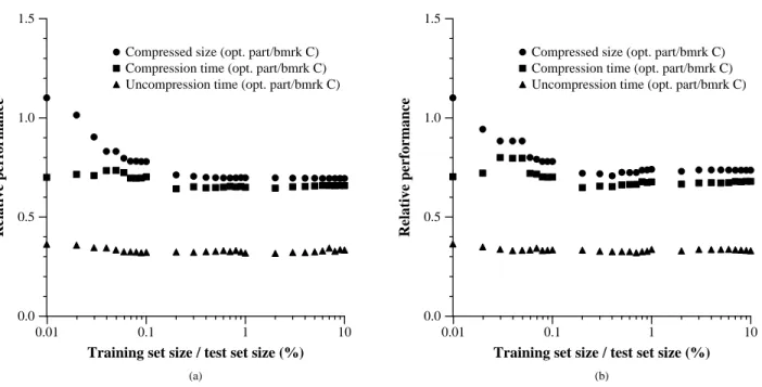
Optimum Partitioning. To test assumption (1) and
as-sess how optimum partitioning affects compression perfor-mance, we used pin to compute optimum partitions on pieces of the training data of increasing size. We ranpzip with each resulting compression plan on the test set and com-pared the compression time and resulting size to those of the benchmarks; we also compared uncompression times. We performed this experiment using both the ordered and ran-dom training sets.
Figures 1 and 2 displays the results, as a function of the amount of training material used. Training on the 2%-size (w.r.t. the test set 2%-size) data set, at which we see the results stabilize, took about 2.27 CPU minutes. Because we anticipate using the same compression plan with multi-ple tables from a fixed source, though, training should be
1ftp://ftp.cdrom.com/pub/infozip/zlib
viewed as an off-line procedure. The results suggest that op-timum partitioning offers significant improvement over both benchmarks and thus fail to falsify assumption (1). We saw 30–35% improvement in compression for this application. We suspect that most of the 15–25% degradation in com-pression and uncomcom-pression time vs. benchmark R can be attributed to the work required for pzip to organize the columns. Analogous effort is required to compress bench-mark C, but not benchbench-mark R. We argue in Section 5 that the resulting size improvement is worth this time overhead.
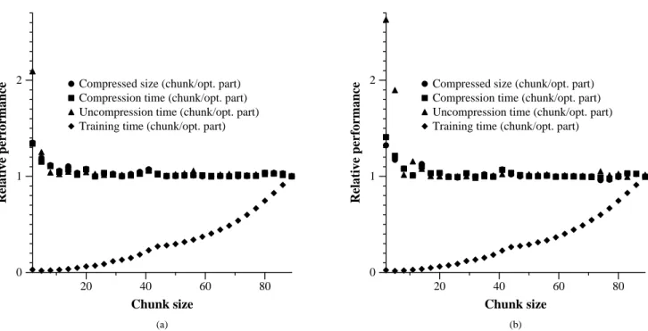
Chunk Partitioning. To test assumption (2) and assess
the degradation in partition quality from using chunk parti-tioning, we computed chunk partitions on the training sets that were 2% of the test set size. (The optimum partition-ing experiment suggests that larger trainpartition-ing sets offer no in-creased benefits in compression performance.) Usingpin on the individual chunks, we computed an optimum chunk partition for each possible chunk size. We usedpzipwith each resulting compression plan to compress the test set. We compared each result to that given bypzipusing an opti-mum partition (from the 2% training size), measuring rel-ative output size, compression and uncompression speeds, and training time. We performed this experiment using both the ordered and random training sets, comparing chunk par-titioning to the corresponding optimum partition.
Figure 3 displays the results, as a function of chunk size. The results fail to falsify assumption (2) and furthermore suggest that chunk partitioning is worthwhile, as small chunk sizes (10–20 in this experiment) yielded almost identical performance as optimum partitioning, but required only about 2–6% of the training time.
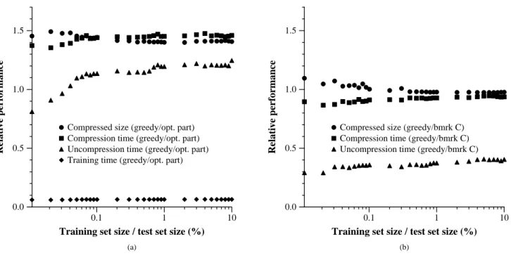
Greedy Differential Compression. To test assumption
(3) and assess how greedy differential compression affects performance, we computed greedy differential compression plans using colsel on pieces of the training data of in-creasing size. We compressed the test set usingcszipwith the resulting plans and compared the resulting size, compres-sion and uncomprescompres-sion time to that ofpzipusing an opti-mum partition (from the 2% training size) and also to bench-mark C. For the comparison to optimum partitioning, we also compared the time to compute the greedy assignment (using
colsel) to that to compute the optimum partition (using
pin). We performed this experiment using both the ordered and random training sets.
0.01 0.1 1 10
Training set size / test set size (%)
0.0 0.5 1.0 1.5
Relative performance
(a)
Compressed size (opt. part/bmrk R) Compression time (opt. part/bmrk R) Uncompression time (opt. part/bmrk R)
0.01 0.1 1 10
Training set size / test set size (%)
0.0 0.5 1.0 1.5
Relative performance
(b)
Compressed size (opt. part/bmrk R) Compression time (opt. part/bmrk R) Uncompression time (opt. part/bmrk R)
Figure 1: Results of optimum partition compression, as a function of amount of training material. Shown is the relative performance of optimum partitioning over benchmark R in terms of compressed size, compression time, and uncompression time. (a) Ordered training set; (b) random training set.
in training time.
We offer a caveat: pzip has undergone significantly more code optimization than cszip, which partially ex-plains the relative difference in running times. We believe that we can improve the running time ofcszipby combin-ing the column differenccombin-ing and compression of the derived columns into a single pass.
4.3 General Discussion. In all the experiments above, the
difference between using ordered and random training sets was negligible, although the ordered sets did provide slightly better results, suggesting the need for future experiments to assess the effects of contiguity in the training data.
We did observe stabilization of compression perfor-mance in all the experiments. Perhaps most remarkable is that this stabilization occurred at training set sizes of 1–2% of the test set size. Again, further experiments with increas-ingly larger test sets and a fixed training set size are required before assumption (4) can be assumed with confidence.
4.4 Comparison to Other Methods. We compared the
result of optimum partitioning (using the 2% training size) to Burrows-Wheeler [1] and PPM [6, 19] compression in isolation. For Burrows-Wheeler, we used Seward’sbzip2, version 0.9.5d.2 For PPM, we used Bloom’sppmz, version
2http://sourceware.cygnus.com/bzip2/index.html
Table 1: Comparison to other methods. Size and times are ratios of optimum partitioning values to the corresponding other-method values.
Compress. Uncompress.
Method Size time time
gzip
row-major 6.340e-1 1.202e-0 1.129e-0 col-major 6.977e-1 6.457e-1 3.168e-1
bzip 7.768e-1 4.344e-1 2.165e-1
PPM 8.786e-1 2.950e-3 4.010e-4
9.1;3 we used coder 9, which offers the best (albeit the
slowest) compression, with the rationale that if best PPM compression turned out to be less than that of optimum partitioning, faster PPM variants would not offer interesting comparisons.
Table 1 details the results. For completeness, we include comparisons togzipused in row-major order (i.e., bench-mark R), corresponding to off-the-shelf use ofgzip, and to gzipin column-major order (i.e., benchmark C). Optimum partitioning achieved greater compression than all the other methods used in isolation. Furthermore, it was faster than all the other methods, except for row-majorgzip; compared to
3http://www.cco.caltech.edu/
0.01 0.1 1 10
Training set size / test set size (%)
0.0 0.5 1.0 1.5
Relative performance
(a)
Compressed size (opt. part/bmrk C) Compression time (opt. part/bmrk C) Uncompression time (opt. part/bmrk C)
0.01 0.1 1 10
Training set size / test set size (%)
0.0 0.5 1.0 1.5
Relative performance
(b)
Compressed size (opt. part/bmrk C) Compression time (opt. part/bmrk C) Uncompression time (opt. part/bmrk C)
Figure 2: Results of optimum partition compression, as a function of amount of training material. Shown is the relative performance of optimum partitioning over benchmark C in terms of compressed size, compression time, and uncompression time. (a) Ordered training set; (b) random training set.
PPM, the relative speed difference was orders of magnitude. The results suggest that, for our table application, opti-mum partitioning usinggzipas the underlying compression method outperforms isolated usage ofbzipandPPM, which by themselves purport to outperform gzip. Since bzip did out-compress gzipwith only a slight time penalty, it is worth future experimentation to assess the performance of optimum partitioning usingbzipas the underlying com-pression method.
5 Partition Compression System and Applications
Pin andpzipactually form our production compression system. Recall that the experiments in Section 4 used only the 90 highest frequency columns from the original data set. Prior to determining an optimum partition, pincalculates column frequencies. It actually computes the optimum par-tition only on the projection of the high frequency columns. (How it determines low from high is a heuristic outside the scope of this paper.) Furthermore, before computing the par-tition, it employs another heuristic to reorder the high fre-quency columns to improve compression size further. Again, this heuristic is outside the scope of this paper and was turned off for the experiments in Section 4.
Pzipthen compresses the low frequency columns by differential encoding, additionally gzipping the output of of that phase, and the high frequency columns with respect to the (reordered) partition. On the low frequency columns of the full network traffic data set, this method outperformed the
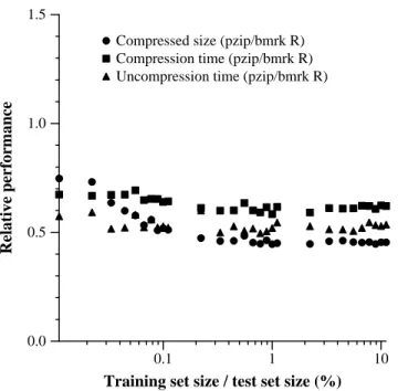
gzipbenchmark (R) by two orders of magnitude in com-pression size and almost an order of magnitude in compres-sion time. To measure how the full system works on the original data set, we repeated the structure of the optimum partitioning experiment, allowingpinto detect the low fre-quency columns andpzipto use differential encoding on them. The system setup was as in Section 4, and again we fixedgzipas the underlying compression method. We com-pared to benchmark R, corresponding to off-the-shelf use of gzip, which was the method of choice in the AT&T net-work traffic data warehouse prior to our net-work. The results are shown in Figure 5. For this experiment, we used only the ordered training set, as the random training set destroys the frequency information.
20 40 60 80
Chunk size
0 1 2
Relative performance
(a)
Compressed size (chunk/opt. part) Compression time (chunk/opt. part) Uncompression time (chunk/opt. part) Training time (chunk/opt. part)
20 40 60 80
Chunk size
0 1 2
Relative performance
(b)
Compressed size (chunk/opt. part) Compression time (chunk/opt. part) Uncompression time (chunk/opt. part) Training time (chunk/opt. part)
Figure 3: Results of chunk partition compression, as a function of chunk size. Shown is the relative performance of chunk partitioning over optimum partitioning in terms of compressed size, compression time, uncompression time, and training time. (a) Ordered training set; (b) random training set.
5.1 Additional Test Sets.
The AT&T network switch statistics project. In this
project, statistics are collected at 15-minute intervals from ATM switches in a network. A record corresponds to a re-placeable circuit component in one of the switches and con-sists of a 16-byte hardware identifier, a 4-byte statistic iden-tifier, a 4-byte time stamp, and a 4-byte count value. Each 15-minute interval produces a file with about 80,000 records for a 6-switch network. The items are sorted by the 16-byte hardware identifier; sorted identifiers usually differ by one byte from one item to the next. The file format is determined by the switch manufacturer and has an irregular structure: variable length headers and interspersed sequencing records make the records variable length in general. The average file size is about 2.2 MB andgzips to about 192 kB, making the daily space requirement 18.4 MB.
To use pzip, each record was padded to a fixed 32 bytes. This expanded the average file size to about 2.6 MB. Training data produced 10 high frequency columns, for which an optimum (reordered) partition was generated. The resulting average pzipped file size was 10.3 kB, for a daily space requirement of 1 MB, a 95% improvement over straightgzip. Compression and uncompression time improvement was only about 20%.
U.S. census data. We took a portion of the United States
1990 Census of Population and Housing Summary Tape File 3A (a.k.a. STF3A) [2]. The data format is fixed length ASCII records. We used field group 301, level 090, for all states.
Table 2: Summary of results. Size and times are ratios of pzipvalues to the correspondinggzipvalues.
Compression Uncompression
Data Size time time
Ntwk. traffic .45 .62 .54
Ntwk. switch .05 .80 .80
U.S. census .56 .50 .33
This generated a 342 MB file with 932-byte records. Gzip compressed the file to 31.5 MB.
Pindetermined that 186 columns were high frequency. In the optimum partition generated, the largest class was 56 bytes wide, indicating high combinational dependence. Pzipcompressed the file to 17.5 MB, a 44.4% improvement overgzip. The compression time improvement was 50%, and uncompression time improvement was 67%.
5.2 Discussion. Table 2 summarizes the results in this
section.
0.1 1 10
Training set size / test set size (%)
0.0 0.5 1.0 1.5
Relative performance
(a)
Compressed size (greedy/opt. part) Compression time (greedy/opt. part) Uncompression time (greedy/opt. part) Training time (greedy/opt. part)
0.1 1 10
Training set size / test set size (%)
0.0 0.5 1.0 1.5
Relative performance
(b)
Compressed size (greedy/bmrk C) Compression time (greedy/bmrk C) Uncompression time (greedy/bmrk C)
Figure 4: Results of greedy differential compression, as a function of amount of ordered training material. (a) Shows the relative performance of greedy differential compression over optimum partitioning in terms of compressed size, compression time, uncompression time, and training time. (b) Shows the relative performance of greedy differential compression over benchmark C in terms of compressed size, compression time, and uncompression time.
can help assess assumption (4), because going forward, pzipwill be compressing an arbitrary amount of data based on the fixed-size training set.
6 Concluding Remarks
We have presented massive tables as a new focus in data compression research. We have given a systematic approach for solving the problem, based on the experimental vali-dation of data dependency assumptions. The result is a new compression paradigm: training for lossless compres-sion. By exploiting data dependencies, our scheme outper-forms standard methods based on information theoretic re-sults, e.g., Lempel-Ziv [20, 21]. We tested two such depen-dencies. For our application, optimum partitioning is better, and it is in production use within AT&T, in thepzip sys-tem. We anticipate instances for which the differential ap-proach will outperform the combinational apap-proach and also instances that favor a hybrid approach. We leave as an open problem to find other data dependencies.
Our results demonstrate the utility of training for loss-less compression. Given multiple tables from a common source, training becomes an off-line operation, suitable for computationally expensive optimizations. The bottleneck in our dynamic programming algorithm for optimum partition-ing is the computation ofS(T[j;i℄)for all1j i n, which requires running the base compressor (gzip, in our case) on(n
2
)intervals of columns. A quick way to
esti-mate the compressed size of an interval of columns, such as providing a suitable lower bound on their joint entropy—a fundamental problem of independent interest—would there-fore be valuable in speeding the overall algorithm.
Two aspects of our work that are now only heuristic are as follows. Permuting the columns before partitioning them effects greater compression. The problem of optimally per-muting the columns can be abstracted in combinatorial op-timization terms as versions of the Hamiltonian path prob-lem or clustering. We suspect that these formulations will prove to be hard, but proving their hardness is non-trivial. Any reduction must capture required costs by constructing columns whose compressed size using a particular program (such asgzip) will match required costs in the reduction. From a practical point of view, an efficient heuristic with good performance is desirable. Our second heuristic involves the choice of low frequency columns that are removed prior to training. In our data sets, simple rules of thumb sufficed to identify such columns, but a formal approach would be desirable.
0.1 1 10
Training set size / test set size (%)
0.0 0.5 1.0 1.5
Relative performance
Compressed size (pzip/bmrk R) Compression time (pzip/bmrk R) Uncompression time (pzip/bmrk R)
Figure 5: Results of usingpin/pzipwith all heuristics and optimum partition compression, as a function of amount of ordered training material. Shown is the relative performance of pzip over benchmark R in terms of compressed size, compression time, and uncompression time.
of using other approximations to the metric facility location problem [3, 11], and to explore hybrid approaches in which we apply optimum partitioning and differential compression to disjoint intervals ofT.
Our experimental methodology—assuming dependen-cies, deriving algorithms based on them, and testing to sup-port or falsify them—may be applied to other compression-based scenarios. It remains to conduct the second test of as-sumption (4)—that the amount of training material needed is independent of the size of the test set—by fixing a compres-sion plan for an arbitrarily large amount of test material. The production use ofpzipis providing an uncontrolled version of this experiment that supports the assumption. Finally, as-sessing the impact of data contiguity on training remains to be studied rigorously.
Acknowledgement
We thank the anonymous reviewers for many helpful com-ments.
References
[1] M. Burrows and D. J. Wheeler. A block-sorting lossless data compression algorithm. Technical Report 124, DEC SRC, May 1994.
[2] Census of population and housing, 1990: Summary tape file 3 on CD-ROM. U.S. Bureau of the Census, Washington, 1992.
[3] M. Charikar and S. Guha. Improved combinatorial algo-rithms for the facility location and k-median problems. In Proc. 40th IEEE FOCS, pages 378–88, 1999.
[4] F. A. Chudak. Improved approximation algorithms for unca-pacitated facility location. In Proc. 6th IPCO, volume 1412 of LNCS, pages 180–94. Springer-Verlag, 1998.
[5] F. A. Chudak and D. B. Shmoys. Improved approximation algorithms for the uncapacitated facility location problem. Unpublished manuscript, 1998.
[6] J. G. Cleary and I. H. Witten. Data-compression using adaptive coding and partial string matching. IEEE Trans. Comm., 32(4):396–402, 1984.
[7] G. Cormack. Data compression in a data base system. C. ACM, 28(12):1336, 1985.
[8] J. Goldstein, R. Ramakrishnan, and U. Shaft. Compressing relations and indexes. In Proc. 14th Int’l. Conf. on Data Eng., pages 370–9, 1998.
[9] D. A. Huffman. A method for the construction of minimum-redundancy codes. Proc. IRE, 49(9):1098–101, 1952. [10] J. J. Hunt, K.-P. Vo, and W. F. Tichy. An empirical study
of delta algorithms. In IEEE Software Configuration and Maintenance Wks., 1996.
[11] K. Jain and V. V. Vazirani. Primal-dual approximation algo-rithms for metric facility location andk-median problems. In Proc. 40th IEEE FOCS, pages 2–13, 1999.
[12] J.-H. Juang, D. Y. Wong, and A. H. Gray, Jr. Distortion performance of vector quantization for LPC voice coding. IEEE Trans. Acous., Spch., and Sig. Proc., ASSP-30(2):294– 304, 1982.
[13] B. Kobler, J. Berbert, P. Caulk, and P. C. Hariharan. Archi-tecture and design of storage and data management for the NASA Earth Observing System Data and Information Sys-tem (EOSDIS). In Proc. 14th IEEE Symp. on Mass Storage Systems, pages 65–76, 1995.
[14] M. Korupolu, G. Plaxton, and R. Rajaraman. Analysis of a local heuristic for facility location problems. In Proc. 9th ACM-SIAM SODA, pages 1–10, 1998.
[15] J. D. Markel and A. H. Gray, Jr. Linear Prediction of Speech. Springer-Verlag, 1976.
[16] A. Moffat. Implementing the PPM data-compression scheme. IEEE Trans. Comm., 38(11):1917–21, 1990.
[17] D. Shmoys, E. Tardos, and K. Aardal. Approximation algorithms for facility location problems. In Proc. 29th ACM STOC, pages 265–74, 1997.
[18] T. A. Welch. A technique for high performance data com-pression. IEEE Computer, 17(6):8–19, 1984.
[19] I. H. Witten, R. M. Neal, and J. G. Cleary. Arithmetic coding for data-compression. C. ACM, 30(6):520–40, 1987. [20] J. Ziv and A. Lempel. A universal algorithm for sequential
data compression. IEEE Trans. Inf. Thy., IT-23(3):337–43, 1977.