DOI 10.1007/s10618-007-0076-8
Collusion set detection using graph clustering
Girish Keshav Palshikar · Manoj M. Apte
Received: 19 May 2006 / Accepted: 17 May 2007 / Published online: 16 June 2007 Springer Science+Business Media, LLC 2007
Abstract Many mal-practices in stock market trading—e.g., circular trading and price manipulation—use the modus operandi of collusion. Informally, a set of traders is a candidate collusion set when they have “heavy trading” among themselves, as compared to their trading with others. We formalize the problem of detection of collusion sets, if any, in the given trading database. We show that naïve approaches are inefficient for real-life situations. We adapt and apply two well-known graph clustering algorithms for this problem. We also propose a new graph clustering algorithm, specifically tailored for detecting collusion sets. A novel feature of our approach is the use of Dempster–Schafer theory of evidence to combine the candidate collusion sets detected by individual algorithms. Treating individual experiments as evidence, this approach allows us to quantify the confidence (or belief) in the candidate collusion sets. We present detailed simulation experiments to demonstrate effectiveness of the proposed algorithms.
Keywords Graph clustering·Clustering·Fraud detection·Collusion set
Responsible editor: Charu Aggarwal.
A preliminary version of this paper was published as Palshikar and Apte (2005). G. K. Palshikar (
B
)Tata Research Development and Design Centre (TRDDC), 54B Hadapsar Industrial Estate, Pune 411013, India
e-mail: [email protected] M. M. Apte
R&D, Engineering and Industrial Services, Tata Consultancy Services, 1 Mangaldas Road, Pune 411001, India
1 Introduction
It is a well-known unfortunate fact that there are unscrupulous organizations and groups of individuals, which attempt to manipulate or influence the activities on stock exchanges with the intention of making profits through illegal or unfair means. Continued prevalence of such mal-practices can have disastrous long-term consequences for the stock exchange, businesses, investors, financial institutions, the government and the economy, in general.
To facilitate fair transactions, the competent authorities keep developing various laws and guidelines (e.g., Securities and Exchange Board (SEBI) gui-delines in India) to be followed by all participants in stock market activities. Enforcing the laws and guidelines requires continuous surveillance of stock market activities through analysis of the associated databases. On-line surveil-lance systems are generally unable to detect or prevent occurrences of complex types of mal-practices because they can only analyse short-term trading data in the limited time available. Such surveillance could be preventive involving early detection and prevention of mal-practices or retroactive involving detection and investigation of suspects and mal-practices in the past.
Many different types of mal-practices may happen in stock market trading. In this paper, we ignore the mal-practices related to payment (e.g., payment default), delivery of shares (e.g., delivery default) etc. We also ignore some trading related mal-practices such as insider trading, takeover bids, market cornering etc. Instead, we focus on specific trading related mal-practices such as circular trading, price manipulation, price hammering, price propping etc.
In price manipulation, a group of individual traders try act together to artificially (and with a view to profit making) attempt to increase the price of a security. This is typically achieved by circulating false information or by creating an artificial demand for the security. To achieve the latter, the traders in the group circulate a fixed number of shares among themselves in a large number of trades; they keep increasing the price in these trades, thereby forcing an increasing trend in the price as well as interesting other traders. When the overall trading price rises sufficiently, the traders in the group “exit” by selling their original shares. Since the price rise was not tenable, the price crashes back to its original level or below. Please refer toPalshikar and Bahulkar (2000)for more details on these mal-practices.
Conceptually, we group these mal-practices together in a class called
collu-sion based mal-practices. This is because all these mal-practices involve a group
The telltale characteristic of the occurrences (or instances) of collusion-based mal-practices is the fact that there is a group of traders, which we call collusion
set, who trade heavily among themselves (in a single security) in the period
under consideration. Different collusion-based mal-practices differ from each other in the trading strategy used during collusion. For example, in circular trading the sequences of trades among the traders in the collusion set are roughly circular. In price manipulation, the trading strategy may be more random i.e., there may not be any specific temporal pattern discernible in the trades among the colluding traders.
The problem that we address in this paper is: how to identify the collusion sets, if any, present in the given trading database? We suggest that identifica-tion of the candidate collusion sets is an important first step in detecting and proving the occurrence of any collusion-based mal-practice. Each candidate collusion set can then be subjected to further in-depth analysis, to establish the occurrence of any collusion-based mal-practice. These follow-up investigations include interviews, analysis of delivery and payment records, raids, prosecution etc., all of which we ignore in this paper.
The difficulties in identifying candidate collusion sets, even for a single known security, are: large size of the trading database, complex sequences of trades, large number of traders, unknown number and identity of the traders in the col-lusion set, and most importantly, subjective nature of the notion of heavy trading (that may vary from security to security, time to time, trader to trader) etc. In addition, various instances of the pattern describing the same mal-practice have similar but not necessarily identical behaviour (or traces) in the trading data-bases. Hence, there is no guarantee that ability to detect one occurrence would be sufficient to detect the other occurrences.
In this paper, we propose the use of graph clustering techniques for efficient detection of candidate collusion sets. Apart from efficiency, this approach has the major advantage that the user does not supply much knowledge; e.g., there is no need to specify the number of candidate collusion sets nor is there any need to quantify the notion of heavy trading.
In Sect. 2, we provide a survey of some related work. In Sect. 3, we de-fine the basic framework of collusion set detection, which includes data pre-paration, the notion of a stock flow graph etc. In Sect. 4, we discuss two well-known graph clustering algorithms and their application to a given stock flow graph for generating candidate collusion sets. In Sect. 5, we discuss an approach to integrate (fuse) the candidate collusion sets, to improve the accu-racy of the candidate collusion sets. Section 6 discusses conclusions and further work.
2 Related work
very difficult to obtain. Hence, we have chosen not to make this assumption for frauds in stock market trading. Thus we need unsupervised learning algorithms that are specialized to separate normal trading from fraudulent trading. There have been a few attempts to formally characterize frauds in stock market tra-ding. Our previous work(Palshikar and Bahulkar 2000)used a fuzzy temporal logic in which users could specify interesting trading patterns. One could apply Hamiltonian circuit enumeration algorithms(Bapeswara Rao and Sankara Rao 1985; Rubin 1974)(or general circuit enumeration algorithms likeHonkanen 1978; Tarjan and Read 1975) to generate all possible candidate collusion sets. However, this is computationally infeasible.
As far as we know, clustering techniques have not been applied to the pro-blem of collusion set detection. Graph clustering is a well-explored field in unsupervised learning in structured domains; we have adapted and applied the two well-known graph clustering algorithmsGowda and Krishna (1978)and Jarvis and Patrick (1973)to the problem of collusion set detection.Jain et al. (1999)provides a general survey of clustering techniques.
Combining multiple statistical classifiers to produce a more reliable classifi-cation is a well-explored problem in statistical pattern recognition.Jain et al. (2000)includes a review of the various classifier combination techniques, which are mostly based on voting and weighted averages. Dempster–Shafer theory of evidence Shafer (1976) is well-known and has been successfully used in many different application domains;Le Hegarat-Mascle et al. (2003)has used it for sensor data fusion. There does not seem to be any work that has used the Dempster–Shafer theory of evidence to combine results of unsupervised
learning algorithms, as we have done in this paper.
3 Collusion set
3.1 Case study
3.2 Naïve approach
We can devise a naïve approach to find candidate collusion sets. Essentially, we generate all subsets of the set traders and check if all traders in the generated subset are “heavily trading” among themselves. If yes, we report the subset as a candidate collusion set. This approach suffers from combinatorial explosion. Also, the notion of heavy trading still needs to be specified by the user. We present polynomial time algorithms to identify candidate collusion sets.
algorithm naive
input trading database D
output collection T of sets of traders
T := set of all traders max := |T| / / no. of traders for m=max, max−1,. . ., 4, 3, 2 do
for every m-subset A of T do
if heavy trade among members of A then report A as candidate collusion set remove A from T
end if end for end for
3.3 Data pre-processing
We assume that the input trading data consists of records having the following (simplified) form:
Stock-ID
Time stamp
Seller-ID
Buyer-ID
Quantity Price Value
Actual trading data contains many other details; e.g., trader details, client details, (sales and purchase) order details such as IDs, placement times, mat-ching time, quantities and prices quoted in the order etc. Each record in this trading database refers to a single trading transaction. Since, these records are timestamped, we can get an idea of the temporal behaviour of the trading. However, our approach to collusion detection does not depend on the detailed temporal aspects of the individual transactions, but only on the overall trading volumes among the traders over a specific time period. Hence, we prepare a summary of the above trading data as follows:
1. Select records for a specific stock, which fall in a specific time period. 2. Summarize the transactions between each pair of seller (trader) and buyer
3.4 Stock flow graph
Definition Using the summary trading database, we construct a directed edge-labelled graph called the stock flow graph for a particular stock-ID S, denoted
GS=(V, E,φ), where V is the set of vertices (each vertex is labelled by a trader
ID), E is the set of directed edges andφis the function that associates a label for each edge. Label of a directed edge(a, b)is the total number of shares sold by a to b (as per the given trading summary database).
A stock flow graph can have parallel edges in opposite directions but cannot have self-loops. It also cannot have any isolated vertices. Stock flow graph can be disconnected. Note that the user has to select the time period for which the summary database is created.
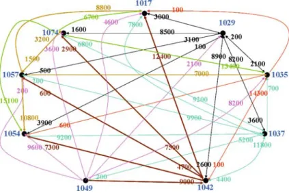
Figure 1 shows an example of a stock flow graph with 9 vertices and 49 edges, where, to avoid clutter, pairs of directed edges (u, v) and (v, u) are shown as single bi-directional edges. The label on an edge (u, v) indicates the total quantity sold by trader u to trader v.
Note that we have defined the stock flow graph to be directed. It is possible to create other varieties of the stock flow graph. For example, we may allow the edges to be undirected and the label of an undirected edge (a, b)is the sum of (i) total number of shares sold by a to b (as per the given trading summary database); and (ii) total number of shares sold by b to a. Alternatively, the sum could be replaced by an absolute difference between (i) and (ii). We prefer the directed stock flow graph, as it more closely matches the intuitive requirements of collusion. For example, in Fig.1, trader 1074 has sold 15,100 shares to 1054 but 1054 has not sold any shares to 1074. So intuitively, when considering collusion sets of size 2, 1054 and 1074 should not be considered. However, if the stock
flow graph were undirected, the edge label between 1054 and 1074 is 15,100, a fairly high edge label in the given example, making it likely that the algorithms may consider them close trading partners. So using undirected stock flow graph may make the collusion detection algorithms more susceptible to influence of large but one-off trades.
4 Graph clustering
A clustering algorithm divides records in a given database into groups or clusters such that records within a cluster are similar to each other and records in different clusters are dissimilar. Each cluster typically corresponds to some concept or class in an application. Clustering algorithms are designed under the unsupervised learning framework, where the attempt is to discover the classes for the given database, with little help from the user. A distance measure is assumed to be available, which gives a numeric value for the dissimilarity between any two records. A clustering algorithm does not need any training or prototype records to be given for each cluster. Moreover, the size, shape and even the number of clusters for a given database are generally unknown. In general, different clustering algorithms discover different clusters, even for the same database i.e., there is no unique grouping of records into clusters.
In our case, since the data to be clustered is a graph, rather than a table of records, we need graph clustering algorithms. The main difference between a database clustering algorithm and a graph clustering algorithm is as follows. Distance can be computed between any two points in the database (e.g., Eucli-dean) whereas for a graph, the distance from a vertex u is available only for the immediate neighbours of u (in the form of labels of outgoing edges from u). Thus graph clustering algorithms are based on the idea that a vertex is likely to belong to the same cluster (or class) as that of its nearest neighbours.
The labelφ(u, v) on a directed edge (u, v) is the total quantity of shares sold
by u to v; thus higher the edge label, closer the vertices in terms of “heaviness” of trading. We will present a simple scheme for distance d(u, v), based onφ(u, v), such that higher the value of d farther the vertices are in terms of “heaviness” of trading. Thus the premise of this paper is: each cluster of vertices identified by a graph clustering algorithm corresponds to traders who trade heavily among themselves. We present experimental evidence of this claim later in the paper.
We apply two different graph clustering algorithms to a given stock flow graph, where the clusters correspond to subsets of the vertices. We then compare the results obtained by these two algorithms.
4.1 Shared nearest neighbour graph clustering
We now describe how we applied the well-known shared nearest neighbour
graph clustering algorithm to the problem of candidate collusion set
Table 1 4NN for vertices in
Fig.1 4NN(1017) =
4NN(1029) =1054, 1037, 1017, 1042 4NN(1035) =1054, 1029, 1017, 1042 4NN(1037) =1054, 1029, 1017, 1074 4NN(1042) =1035, 1017, 1037, 1029 4NN(1049) =1054, 1042, 1035, 1037 4NN(1054) =1029
4NN(1057) =1054, 1037, 1017, 1035 4NN(1074) =1054, 1035, 1037, 1029
minimum no. of common nearest neighbours, explained later). We denote the ordered sequence of k nearest neighbours of a vertex u by kNN(u). Vertices in
kNN(u) are ordered, with the first vertex being the nearest to u; e.g., Table1 shows 4NN for Fig.1.
The algorithm first retains only k outgoing edges for each vertex, one to each of its k nearest neighbours. Then it iteratively compares every pair of vertices
u and v, merging their corresponding clusters, if: (i) u and v share more than kt≤k neighbours; and (ii) u and v are among the k-nearest neighbours of each
other. This continues until there are pairs of vertices that can be merged.
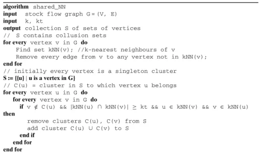
algorithm shared_NN
input stock flow graph G = (V, E)
input k, kt
output collection S of sets of vertices
// S contains collusion sets for every vertex v in G do
Find set kNN(v); //k-nearest neighbours of v
Remove every edge from v to any vertex not in kNN(v); end for
// initially every vertex is a singleton cluster S := {{u}|u is a vertex in G}
// C(u) = cluster in S to which vertex u belongs for every vertex u in G do
for every vertex v in G do
if v ∈/ C(u) && |kNN(u) ∩ kNN(v)| ≥ kt && u ∈ kNN(v) && v ∈ kNN(u) then
remove clusters C(u), C(v) from S add cluster C(u) ∪ C(v) to S end if
end for end for
The above algorithm uses a sub-routine to compute the k-NN list of a vertex
v. In the simplest case, this routine sorts the neighbour of v in the decreasing
slight complication arises when the edge labels for the neighbours of v are not all distinct. In that case, the question is how to resolve the conflicts among the neighbours and pick the k nearest neighbours. We have chosen a simple strategy for this as follows. Suppose L=u1, u2,. . ., uk, uk+1,. . ., umis the sorted list of
v’s neighbours. We pick up the first k neighbours u1, u2,. . ., uk. Now if the
edge label of uk+1is different from that of ukthen we are done. Otherwise, we
keep on adding uk+1, uk+2,. . .until we reach a neighbour whose edge label is different from that of uk(or if we reach the last neighbour um). In general, this
strategy may result in the k-NN list containing more than k elements.
For the stock flow graph in Fig.1, suppose we use k=4 and kt=2.4 nearest neighbours of 1074 and 1042 are:
S1=4NN(1074)= 1054, 1035, 1037, 1029
S2=4NN(1042)= 1035, 1017, 1037, 1029
The sets S1and S2have three traders in common (underlined); so the condition
|S1∩S2| ≥ kt is true. However, 1074 ∈/ 4NN(1042); so S1 and S2 cannot be merged. But
S3=4NN(1029)= 1054, 1037, 1017, 1042
S4=4NN(1037)= 1054, 1029, 1017, 1074
The sets S3and S4have two traders in common (underlined); so the condition
|S3∩S4| ≥kt is true. Also, 1029∈4NN(1037)and 1037∈4NN(1029); so S3and
S4can be merged.
For the stock flow graph in Fig.1, we get the following candidate collusion sets for different values of k and kt. The underlined traders appear in a single collusion set in all of these experiments; hence there is good reason to believe that a likely candidate collusion set is{1029, 1037, 1042, 1074}.
k=5 kt=2
{1029, 1035, 1037, 1042, 1074}
k=6 kt=4
{1029, 1037, 1042, 1074}
k=7 kt=5
{1029, 1037, 1042, 1057, 1074}
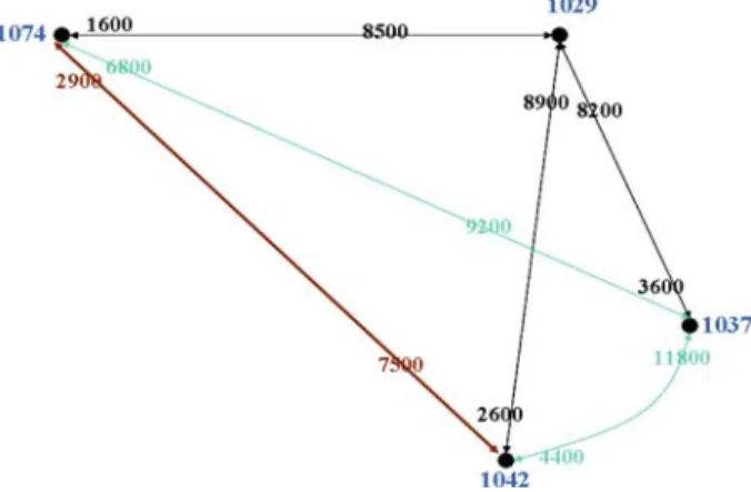
Fig. 2 Subgraph of Fig.1corresponding to the candidate collusion set{1029, 1037, 1042, 1074}
Proposition (Jarvis and Patrick 1973)The complexity of shared-NN graph clu-stering is O(kN2) where N = no. of vertices or traders (and not the number of trades).
Thus it is an efficient algorithm. The algorithm is self-scaling i.e., there is no need to specify the number of clusters, conditions for heavy trading etc. The algorithm obeys the transitivity property: if p shares a lot of points with q and
q shares a lot of points with r then p, q, r tend to belong to the same cluster.
The algorithm can discover clusters of arbitrary shapes and sizes. Empirically, we also found the followingJarvis and Patrick (1973):
1. As kt is increased, keeping k constant, the sizes of the clusters tend to decrease.
2. As k is increased, keeping kt constant, the sizes of the clusters tend to increase.
Typically, the size of the collusion set is small because it is more difficult to manage collusion (particularly, in computerized trading systems) among a large no. of traders. Thus parameters chosen should achieve clusters of size less than a limit identified by domain experts.
4.2 Mutual nearest neighbour graph clustering
We now describe how we applied the well-known mutual nearest neighbour
graph clustering algorithm to the problem of candidate collusion set detection.
This algorithm takes a stock flow graph as input, along with one integer para-meter k. The similarity measure used in this clustering algorithm is based on the concept of mutual neighbourhood value.
For Fig.1(using Table1), mnv(1029, 1037)=2+2=4. If v does not occur in the k-NN list of u then rank of v in u’s k-NN list is defined to be some large constant (e.g., 100). The rank of 1049 in the 4NN list of 1037 is 100; so
mnv(1037, 1049)=100+4=104.
Definition A cluster is a set of vertices. The mnv between two clusters (for a given k) is defined as the maximum mnv between any pair of points in the combined cluster.
Thus the mnv between clusters{1029, 1054}and{1035, 1042} =max{mnv(1029, 1035), mnv(1029, 1042), mnv(1054, 1035), mnv(1054, 1042)} =max{102, 8, 101, 200} =200.
In our experiments, we found that using maximum mnv between any pair of points in two clusters does not yield good results.
Definition We (re)define the mnv between two clusters (for a given k) as the average mnv between any pair of points in the combined cluster.
The idea of using average is similar to that in average linkage clustering. Thus the mnv between clusters{1029, 1054}and{1035, 1042} =average{mnv(1029, 1035), mnv(1029, 1042), mnv(1054, 1035), mnv(1054, 1042)} = average{102, 8, 101, 200} =411/4=102.75.
algorithm mutual_NN_avg
input k, m // m = desired no. of clusters
input stock flow graph G = (V, E)
output collection S of sets of vertices
// S contains collusion sets for every vertex v in G do
Find set kNN(v); //k-nearest neighbours of v
Remove every edge from v to any vertex not in kNN(v); end for
// initially every vertex is a singleton cluster S := {{u}|u is a vertex in G}
while |S|>m do
find two cluster C1 and C2 such that mnv(C1,C2) is minimum among all pairs of clusters
(use lowest inter-cluster distance in case more than one pairs of clusters have the same mnv)
minimum_mnv = mnv(C1,C2)
if minimum_mnv >=MAX_MNV then break end if ; remove clusters C1, C2 from S
add cluster C1 ∪ C2 to S end while
The algorithm first retains only k outgoing edges for each vertex, one to each of its k nearest neighbours. Initially, every vertex is a singleton cluster. The algorithm then iteratively compares every pair of clusters Ciand Cj,
It then merges the selected pair of clusters into a single cluster. When two pairs of clusters {C1, C2}and {C3, C4} are such that mnv(C1, C2) = mnv(C3,
C4) then we use inter-cluster distance d(Ci, Cj) to choose. Thus we choose
the pair of clusters{C1, C2}to merge if d(C1, C2) < d(C3, C4). In our work, we defined d in terms of edge weights such that points connected with an edge having more weight are nearer (since edge weight = number of shares sold).
The results of using the mutual nearest neighbour graph clustering algorithm, with our modifications, on Fig.1are as follows:
k=2{1029, 1037, 1054}
k=3{1029, 1037, 1054}{1035, 1042}
k=4{1029, 1037, 1054, 1074}{1035, 1042}
k=5{1029, 1035, 1037, 1042, 1054, 1074}
Since traders 1029, 1037, 1054 always occur in the same cluster for different values of k, we suggest that{1029, 1037, 1054}is a candidate collusion set.
Proposition (Gowda and Krishna 1978) The complexity of this algorithm is O(kn2) where n is the number of vertices (traders) in the stock flow graph.
This algorithm is self-scaling i.e., there is no need to specify in advance conditions for heavy trading, the number of clusters (m can always be given as 1, since the algorithm stops if the clusters are far apart as controlled by the condition minimum_mnv>= MAX_MNV) etc. The algorithm can discover clusters of arbitrary shapes and sizes. As k is increased, the number and size of the discovered clusters tends to increase(Gowda and Krishna 1978).
4.3 Collusion clustering
We now present a new clustering algorithm specifically tailored for the problem of detection of candidate collusion set. Recall that we informally defined a collusion set as that set of traders who trade heavily among themselves and relatively less with others. We now formalize this definition with a view towards using it in a clustering algorithm.
Definition For a set of traders C, the internal trading of C, denoted I(C), is the sum of the quantity in all trades where both the buyer and seller are in C i.e.,
I(C)=
u∈C,v∈C
q(u, v)
Definition External trading E(C)of a set of traders C is the sum of the quantity in all trades where either the buyer or the seller (but not both) are in C i.e.,
E(C)=
u∈C,v∈/C
q(u, v)+
u∈/C,v∈C
q(u, v)
Definition The collusion indexφ(C)of a set C of traders is defined as the ratio φ(C)=I(C)/E(C). If a trader does not trade with itself (e.g., on behalf of two different customers) then the collusion index of a singleton set is always zero.
In Fig.1, the collusion index ofφ({1029, 1037, 1074})=37900/129800≈0.29. It is easy to see thatφis a monotonically increasing function i.e., as the size of the set C increases, the value of its collusion indexφ(C)increases. Formally, if
D⊆C thenφ(D)≤φ(C). This follows from the fact that internal trading of C is>that of D and external trading of C is less than that of D.
Definition Suppose C1and C2are two disjoint sets of traders. We define col-lusion level Lc(C1, C2) between them as the collusion index of C1∪C2 i.e.,
Lc(C1, C2) = φ(C1 ∪C2). Thus higher values of Lc(C1, C2) indicate better chances that C1∪C2is a candidate collusion set.
For example, the collusion level of two clusters {1029} and {1037, 1074} is φ({1029, 1037, 1074}) = 0.29. Clearly, Lc(C1, C2) ≥ 0. However, Lc(C, C) is
not necessarily zero, because in general the internal trading of the traders in C will be non-zero. It is easy to see that Lc(C1, C2)=Lc(C2, C1). This is because the internal and external trading of C1∪C2is the same as that of C2∪C1. Definition Let S= {C1, C2,. . ., Cn}be a collection of clusters. Then maximum
similarity in S, denotedα(S), is defined as the maximum value of Lc(Ci, Cj), over
all possible combinations of 1 ≤i, j≤n (i.e., over all combinations of distinct
clusters in S); i.e.,α(S)=max{Lc(Ci, Cj)|1≤i, j≤n, i=j}. Two clusters Ciand
Cjin S are most similar in S if Lc(Ci, Cj)=α(S)i.e., Ciand Cjare most similar
among all pairs of clusters in S.
For example, when S includes nine singleton clusters (one for each vertex in Fig.1), the maximum similarityα(S)=Lc({1054},{1074})=0.14.
Definition Given 2 integers m and k, 1≤m≤k, and two clusters C and D, a
point p in C is(k, m)-compatible with D if kNN(p)contains at least min (m,|D|) points.
Definition Given two integers m and k, where 1≤m≤k, and real number 0≤ h≤100, two clusters C and D are (k, m, h)-compatible (or simply, compatible) if at least h%points in C are(k, m)-compatible with D and at least h%points in
D are(k, m)-compatible with C.
algorithm collusion_clustering
input k, m, h
input stock flow graph G = (V, E)
output collection S of sets of vertices
// S contains collusion sets for every vertex v in G do
Find set kNN(v); //k-nearest neighbours of v
Remove every edge from v to any vertex not in kNN(v); end for
// initially every vertex is a singleton cluster S := {{u}|u is a vertex in G}
while (1) do
Let B := ordered sequence of all pairs of clusters in S, sorted in descending order of Lc values
for every pair of clusters (C,D) in B do
if Lc(C, D) > 0 and C and D are (k,m,h)-compatible then remove C, D from S
add C ∪ D to S break;
end if end for end while
with 1042. We now define a simple clustering algorithm that uses collusion level as the similarity measure to merge clusters.
The algorithm starts by making every point a singleton cluster. Iteratively it finds and merges that pair of clusters which are (i) (k, m, h)-compatible and (ii) have the highest value of the collusion level Lc. It stops when no pair of
(k, m, h)-compatible clusters can be found or when the Lcvalue is 0 for all pairs
of clusters. Note that the user does not have to provide the desired number of clusters.
Proposition The complexity of the algorithm is O(kn3), where n=number of vertices in the stock flow graph (i.e., no. of traders) and k =number of nearest neighbours retained for each vertex.
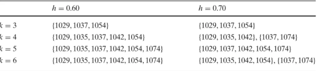
Table2shows the results yielded by the algorithm for the stock flow graph in Fig.1:
Suppose k=4, m=1, h=0.70. Initially, S consists of nine singleton clusters, one for each vertex in Fig.1. Since Lc({1035},{1042}) is maximum among the
Table 2 Results for stock flow graph in Fig.1(m=1)
h=0.60 h=0.70
k=3 {1029, 1037, 1054} {1029, 1037, 1054}
k=4 {1029, 1035, 1037, 1042, 1054} {1029, 1035, 1042},{1037, 1074}
k=5 {1029, 1035, 1037, 1042, 1054, 1074} {1029, 1037, 1042, 1054, 1074}
(4, 1, 0.7)-compatible points, the first pair of clusters to be merged is{1035}and
{1042}. The sequence in which clusters are merged is as follows:
{1035}merged with{1042}
{1029}merged with{1035, 1042}
{1037}merged with{1074}
Some empirical observations about the behaviour of the algorithm are as follows.
1. The algorithm is very sensitive to the value of m. Usually, m=1 is the most useful value i.e., when merging clusters C and D, each point in C should have at least 1 k-NN in D and vice versa. Checking for more than 1 k-NN is too strict a condition, leading to early failure in merging the clusters and thereby stopping the algorithm early.
2. As k increases (for fixed m and h), the size and the number of clusters tends to increase. Since, larger k allows us to examine more neighbours, the possibility of merging increases, leading to larger clusters.
3. As h increases (for fixed m and k), the size and the number of clusters tends to decrease. Larger value of h implies that (k, m, h)-compatibility is checked for more points in clusters C and D, increasing chances of failure to merge which leads to smaller clusters.
4. Traders who engage predominantly in buying (accumulators) (e.g., 1017, 1054) or predominantly in selling (e.g., 1049) generally tend to get omitted from the clusters. This is desirable, since a colluder should interact as both buyer and seller with his partners.
4.4 Using multiple factors
We have so far assumed that every edge label consists of only one value viz., the total volume. In real-life applications, there may be a need to take multiple fac-tors into account when identifying the collusion sets. For example, we may wish to use the total number of trades as an additional factor, based on the intuitive idea that colluding entities may trade more frequently among themselves (e.g., to escape attention from single large volume trades).
We now present a simple modification of the graph clustering algorithms presented earlier in this paper to use multiple value components in edge labels. For simplicity, we assume that edge label has two value components: volume and number of trades (generalization to more than two values is simple). Each vertex now has two separate k-NN lists, one for each value component in edge label. For example, in the stock flow graph in Appendix A, the 4-NN lists for vertices 1029, 1037, 1074 using only volume as the edge weight are as follows:
4NN(1074)= 1054, 1035, 1037, 1029
The 4-NN lists for these vertices, using only trade count as the edge label are as follows:
4NN(1029)= 1054, 1037, 1042, 1017 4NN(1037)= 1017, 1054, 1029, 1074 4NN(1074)= 1054, 1029, 1042, 1035
Using only volume and kt=2, vertex 1029 can merge with 1037, and vertex 1037 can merge with 1074. However, using only trade as the edge weight, vertex 1029 can merge with 1037, but vertex 1037 cannot merge with 1074.
Basic question now is how to deal with these two separate two separate criteria (and the associated k-NN lists). We propose one possible way for the shared-NN algorithm as follows. We merge two clusters if and only if both k-NN lists satisfy the merging criteria specified in shared-NN algorithm. Formally, the shared-NN algorithm now uses the following criteria for merging vertices u and v:
|kNN1(u)∩kNN1(v)| ≥kt &&
|kNN2(u)∩kNN2(v)| ≥kt && u∈kNN1(v) && v∈kNN1(u) && u∈kNN2(v) && v∈kNN2(u)
Here, kNN1(x)and kNN2(x)indicate the k-NN lists of vertex x for volume and number of trades, respectively. We have implemented the shared-NN algo-rithm modified to take into account multiple edge labels according to the above criteria. For the example stock flow graph in Appendix A, the shared-NN algo-rithm identifies the following candidate collusion sets:
k=5 kt=2
{1029, 1035, 1037, 1042, 1074}
k=6 kt=4
{1029, 1037, 1042, 1074}
k=7 kt=5
{1029, 1037, 1042, 1049, 1057, 1074}
There are other ways in which the two k-NN lists can be used to define the merging criteria. For example, we may combine the two k-NN lists into a single
k-NN list as follows. For each vertex, associate the sum of ranks of that vertex
in both the k-NN lists. Then we pick top k of these vertices as the final k-NN list. In our earlier example,
4NN2(1037)= 1017, 1054, 1029, 1074
The rank of the various vertices are:
Rank(1054)=1+2=3 Rank(1029)=2+3=5 Rank(1017)=3+1=4 Rank(1074)=4+4=8
Thus the combined k-NN list is:
4NN1(1037)= 1054, 1017, 1029, 1074
We need a criteria to resolve conflicts that occur due to the same rank values for two or more vertices (we omit it here).
5 Combining the results
We presented three different algorithms to detect collusions sets in given trading database. The basic ambiguity stems from the fact that there is no formal and effective (i.e., executable) definition of what constitutes a collusion. It can be observed that the three algorithms give somewhat different results, when called with different parameter values. We now address the question of whether it is possible and useful to formally combine the results of these algorithms to arrive at a more confident estimate of the actual collusion sets.
This situation is somewhat similar to the well-known classifier combination problem in the pattern recognition community. There different classifiers are constructed from the same training data; e.g., the classifiers may be a decision tree, a neural network and a support vector machine. When the same unseen test example is given to these different classifiers, the results are not always unanimous. Different combination schemes, typically based on voting mecha-nisms, are used to combine the class labels suggested by the different classifiers to arrive at the final class label for the test example.
In this paper, we propose to use the Dempster–Shafer theory of evidence to combine the collusion sets generated by these three algorithms to arrive at a more confident estimate of the actual collusion sets.
5.1 Overview of Dempster–Schafer theory of evidence combination
the strength of evidence in favour of s. Bel(s)=0 (respectively, 1) means we have no evidence (respectively, absolute evidence) in favour of s. Pl is the
plausibility which measures the extent to which evidence in favour of¬s leave
room for belief in s. Pl is defined as
Pl(s)=1−Bel(¬s)
Both Bel and Pl can take real values from 0 to 1. For example, if we have absolu-tely convincing evidence in favour of¬s, then Bel(¬s)=1 and hence Pl(s)=0. Let , called the frame of discernment, denote the set of all possible hypo-theses. For example, if T= {1017, 1029, 1035, 1037, 1042, 1049, 1054, 1057, 1074} is the set of nine traders, then is the collection of all possible subsets of
T; thus contains 29 elements. Here, a hypothesis is a subset of T, which is suspected of being a collusion set. Initially, every element of(i.e., every subset of T) has an interval [0, 1] associated with it, indicating that we have no evidence in favour of (or against) any hypothesis. Our goal is to attach a measure of belief with each element of . Often, an evidence supports a set of hypotheses, rather than a single hypothesis. In our example, when we run the mutual_NN algorithm with k = 3, we get two candidate collu-sion sets {1029, 1037, 1054} and {1035, 1042}, i.e., this algorithm has genera-ted evidence against the subset of hypotheses{{1029, 1037, 1054},{1035, 1042}}. Instead of Bel and Pl, we compute a belief function m, where m(p)measures the belief currently assigned to the subset p ⊆. The function m is defined such that the sum of m values for all 2|| subsets of is 1. For p ⊆ , Bel(p) can be expresses in terms of m: Bel(p)is the sum of the values of m for p and for all its subsets. Bel(p) is our overall belief that the correct hypothesis is in p. At the core of Dempster–Schafer theory is the rule that allows com-bining evidence from two different sources. Suppose we are given two belief functions m1and m2. Let X be the set of subset of to which m1 assigns a non-zero value and let Y be the corresponding set for m2. Then the combina-tion of belief funccombina-tions m1and m2results in a new belief function m3defined as:
m3(Z)=
X∩Y=Zm1(X)·m2(Y)
1−X∩Y=∅m1(X)·m2(Y)
Once we define how to map the results (i.e., set of candidate collusion sets) to a belief function, then we can use the above rule to combine the results of two algorithms and arrive at a new combined belief function.
5.2 Combining evidence from multiple collusion sets
of all Hamiltonian circuits in G. Letω(HˆG)denote the largest weight among
weights of all Hamiltonian circuits inHˆG.
Definition Let G be a given stock flow graph. Let C be a given set of traders (subset of vertices in G). Let G(C)denote the subgraph of G induced by vertices in C. Case (i): G(C)is Hamiltonian. Then the collusion coefficient of C, denoted γ (C), is defined as the ratioγ (C)=ω(HˆG(C))/I(C), whereω(HˆG(C))is as defined
above and I(C)is the internal trading of C. Case (ii): G is not Hamiltonian. Let denote the set of all Hamiltonian circuits of maximum size among all subgraphs of G(C). If= ∅then the collusion coefficient of C, denotedγ (C),
is defined as 0; otherwise, it is defined as the ratioγ (C)=ω()/I(C).
Let G denote the stock flow graph in Fig.2; G is Hamiltonian. The weight
w(1029, 1037, 1074, 1042, 1029) = 3, 600 whereas w(1029, 1037, 1042, 1074, 1029) = 2, 900. It is easy to see that ω(HˆG) = 3, 600 i.e., there is no
Ha-miltonian circuit in G having larger weight. The set of vertices in Fig. 2 is
C= {1029, 1037, 1042, 1074}. Thenγ (C)=3, 600/76, 000=0.047.
Let T be the set of all traders in the given database; In Fig.1, T = {1017, 1029, 1035, 1037, 1042, 1049, 1054, 1057, 1074}. Let=2Tdenote the power of T i.e., the set of all subsets of T. Each element ofis a hypothesis i.e., a potential collusion set. Let m denote the belief function over. Let p be a subset of i.e., p contains zero or more subsets of T. m(p)is the amount of belief currently assigned to the set p of hypotheses. Initially, before any experiments with the three algorithms are done, we assign a belief of 1.0 to.
{} (1.0)
Suppose we run the shared_NN algorithm on the data in Fig. 1 with k = 6 kt =4, getting the candidate collusion set A = {1029, 1037, 1042, 1074}. We propose to use the collusion coefficientγ (A)as a measure of belief that A is a collusion set. We treat results of one run of an algorithm as evidence. This results in an update of m1as follows:
{1029, 1037, 1042, 1074} (0.047)
{} (0.953)
Suppose we now run the collusion_clustering algorithm with k=3, m=1,
h=0.70, getting the candidate collusion set{1029, 1037, 1054}. This results in a new m2function:
{1029, 1037, 1054} (0.004)
{} (0.996)
{1029, 1037, 1054}(0.004)
{}(0.996)
{1029, 1037, 1042, 1074} (0.047)
{1029, 1037} (0.000188)
{1029, 1037, 1042, 1074} (0.046812)
{}(0.953) {1029, 1037, 1054} (0.003812)
{}(0.949188)
We now illustrate the use of the Dempster–Schafer theory (as discussed above) to combine results obtained by all the three algorithms with different parameter values (Fig.3). The idea is to formalize our intuitive understanding that more the experiments that report a trader as part of a candidate collusion set, more is our belief that he is indeed likely to be a colluder.
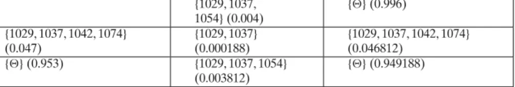
For Fig. 1, we have obtained the results in Table 3. As discussed above, using Table3as input data, we sequentially revise the belief function m (using Dempster–Schafer evidence combination rule) after each experiment.
In Table 3, the set p of hypotheses is obtained by taking the candidate collusion sets in column 4. Actually, p is a multi-set, since the same collusion set can be obtained in different experiments (e.g.,{1029, 1037, 1054}). We start with the belief function m that allocates a belief of 1.0 to the all-inclusive hypothesis = {1017, 1029, 1035, 1037, 1042, 1049, 1054, 1057, 1074}. Successively, revising the belief function after each experiment, we obtain the following final belief function m at the end of these experiments:
Definition Suppose p denotes a set of hypotheses. Then in Dempster–Schafer theory, belief of p, denoted Bel(p), is defined as the sum of the values of the
belief function m for p and for all its subsets.
Using Table4, we obtain the following:
Bel({1029, 1037, 1042, 1074})=0.446140
Bel({1029, 1035, 1037, 1042, 1074})=0.454707
All other collusion sets in Table3have a much less belief value. Thus we can recommend{1029, 1037, 1042, 1074}and{1029, 1035, 1037, 1042, 1074}as candi-date collusion sets. These collusion sets include all other collusion sets reported
shared_NN graph clustering algorithm
mutual_NN graph clustering algorithm Trading
database
collusion graph clustering algorithm
Dempster-Schafer evidence combination candidate
collusion sets
reported candidate collusion sets
Ta b le 3 Candidate collusion sets identified in d ifferent experiments for the graph in F ig . 1 No . A lgorithm Parameters Candidate collusion set C ω(
ˆHG
Table 4 The final belief
function for Table3 0.005990,∅
0.000048,{1029} 0.005009,{1037} 0.000331,{1029,1037} 0.000185,{1042} 0.000188,{1029,1042} 0.414050,{1037,1074}
0.026329,{1029,1037,1042,1074} 0.003757,{1035,1042}
0.003812,{1029,1035,1042}
0.000998,{1029,1035,1037,1042,1074} 0.006446,{1029,1037,1054}
0.532858,{1017,1029,1035,1037,1042,1049,1054,1057,1074}
in Table3, except{1029, 1037, 1054}, which has a very low belief value. These candidate collusion sets can now be investigated further in detail to find actual colluders, if any. Note that because of the combination of results from different algorithms, the recommended collusion set has a higher belief value than in any single experiment.
6 Experimental results
6.1 Performance measurements
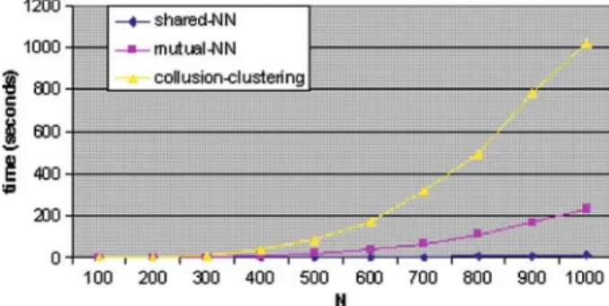
Figure4shows the performance of the three graph clustering algorithms on syn-thetic trading data. We randomly generate stock flow graph, from the following parameter values:
• N (no. of vertices): from 100 to 1,000 in steps of 100 • µd(the average degree for the vertices): 0.15∗N
• µv(average volume (edge label) for the edges): 1000.
We assumed that the degrees of the vertices are distributed exponentially around the given average degreeµd, with the additional restriction that degree of each vertex has to be≤N−1. We also assumed that the volume is distribu-ted exponentially around the given average degreeµv. We used the following
parameters for each of the algorithms:
• shared-NN: k=4, kt=2
• mutual-NN: k=4
• collusion clustering: k=4, m=1, h=0.7.
For each value of N, we generated the stock flow graph 10 times, and averaged the running time of each algorithm over these 10 runs.
6.2 Accuracy of collusion set detection
In the second experiment, we attempted to validate the accuracy of the graph clustering algorithms in detecting known collusion sets. For this purpose, we followed the same procedure as above for generating synthetic data. In addition, we induced one collusion set of known size C in the synthetic data. For a given collusion set of size C (i.e., containing C traders), we selected C vertices and introduced C∗(C−1)edges between every pair of them, each edge labelled with a volume v, drawn from an exponential distribution with mean= 3∗µv. Thus
the collusion set had substantially larger trading within itself, as compared with its trading with others. Moreover, in the generated collusion set S, each trader in
S had trading with every other trader within S. That is, the subgraph induced by
the collusion set is a complete graph (clique). This is most important, because in real life not all colluders may trade with each other. For example, in perfect circularly collusion of size 4, trader A will trade with B, B with C, C with D and D with A; there will not be any other cross-trades among these.
In our experiments, we varied the size C of the induced collusion set from 3 to 10. For shared-NN, k was set to 2∗C and kt was fixed at 2. For mutual-NN, k
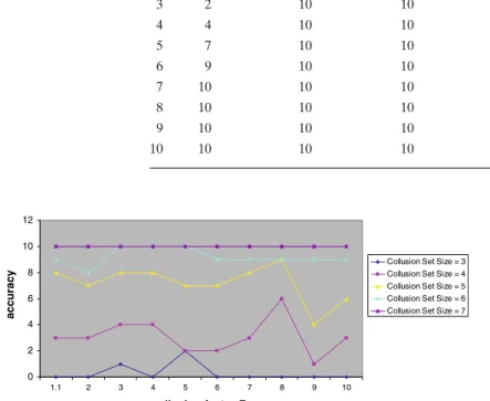
was set to 2∗C. For collusion clustering, k was set to 2∗C, m=1 and h=0.7. For each value of C, we generated the stock flow graph and induced a collusion set of size C and tested whether each graph clustering algorithm was able to detect the induced collusion set (in a single cluster) or not (See Table5). Following table gives, for a specific value of C, the no. of times out of 10, the algorithm detected the collusion set.
6.3 Effect of collusion factor on accuracy of shared_knn
In our data generation scheme, the average volume for normal trading is generated using an exponential distribution with mean =µv. The average
volume for trading among the members of the known collusion set is also exponentially distributed with mean = 3∗µv. We call this number 3 as the
collu-sion factor F. Value of F indicates how significantly the average trading volume
Table 5 Accuracy of graph
clustering algorithms C Shared-NN Mutual-NN Collusion-clustering
3 2 10 10
4 4 10 10
5 7 10 10
6 9 10 10
7 10 10 10
8 10 10 10
9 10 10 10
10 10 10 10
0 2 4 6 8 10 12
1.1 2 3 4 5 6 7 8 9 10
collusion factor F
accuracy
Collusion Set Size = 3 Collusion Set Size = 4 Collusion Set Size = 5 Collusion Set Size = 6 Collusion Set Size = 7
Fig. 5 Accuracy of shared_knn algorithm for varying collusion factor F
to understand the effect of varying the collusion factor F on the accuracy of collusion set detection.
For this purpose, we followed the same procedure as above for generating synthetic data. We varied the collusion factor F from 1.1 to 10.0 and the size
C of the collusion set from 3 to 10. For each such tuple of values for F and C,
we generated the stock flow graph 10 times, and counted the number of times (out of 10) the collusion set was correctly detected by the shared_knn algorithm (this number is called the accuracy). We omit the results for other algorithms because they were almost 100% accurate for almost any combination of these values for F and C.
Figure5shows the accuracy of shared_knn algorithm for different values of the collusion factor F. The accuracy increases with induced collusion set size
C and reaches 100% whenever C is≥7. Note that when the collusion set size is low (e.g., 3 or 4), the accuracy of shared_knn remains low. This happens because the number of neighbours considered increases with C (we are using
on the size of the collusion set C rather than the collusion factor F. That is, the shared_knn algorithm works satisfactorily even if the trading volumes are not significantly higher within the collusion set as compared to trading volumes among other traders (though, of course, they have to be at least slightly higher, which is why the value of F starts at 1.1). Thus neighbourhood-ness among traders is more important than values of trading volume, for collusion set detection.
6.4 Effect ofµdon accuracy of shared_knn
Note that in our earlier experiments, value of k (the number of nearest neigh-bours used) was constant (for a particular value of C =size of the induced collusion set). We now investigate how the accuracy of shared_knn algorithm varies for different values of k, keeping the number of vertices and the size of the induced collusion set constant.
We randomly generate stock flow graphs using the same procedure as des-cribed earlier with N =200,µd =30, kt=2, C=3, 4,. . ., 10. For each value of
C, we vary k from 12 to 28 in steps of 2 and observe the accuracy of collusion
set detection. The shared_knn algorithm tends to be inaccurate when value of
k is less than the expected size of the largest collusion set. Since maximum size
of C is 10 in our experiments, we use values of k from 12 onwards. Since the average number of neighbours for a vertex (µd) is 30 in the generated stock flow
graphs, hence we keep the value of k below 30. In this experiment, we found that the accuracy reaches 100% k ≥ 14 for all values of C. This experiment suggests a heuristic to select the right value of k, when the size Cmaxof the
largest candidate collusion set is known: use k≥Cmax.
6.5 Effect of k on accuracy of shared_knn
The next experiment is designed to understand the effect of changing the density of the stock flow graph from sparse to dense. In our earlier data generation scheme, the average degree of a vertex in the stock flow graph is µd = 30
(which is 0.15∗N, where N=total no. of traders = 200). The next experiment is designed to understand the effect of varying the average degreeµdof the stock
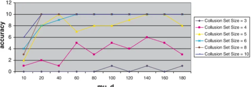
flow graph from 10 to 190 (N = 200 is fixed) on the accuracy of shared_knn algorithm for collusion set detection. As earlier, we have fixed the collusion factor F=3.
We variedµd from 10 to 190 and the size C of the collusion set from 3 to
10. For each such tuple of values forµd and C, we generated the stock flow
graph 10 times, and counted the number of times (out of 10) the collusion set was correctly detected by the shared_knn algorithm (this number is called the
accuracy). We omit the results for other algorithms because they were almost
0 2 4 6 8 10 12
10 20 40 60 80 100 120 140 160 180
mu_d
accuracy
Collusion Set Size = 3 Collusion Set Size = 4 Collusion Set Size = 5 Collusion Set Size = 6 Collusion Set Size = 8 Collusion Set Size = 10
Fig. 6 Accuracy of shared_knn algorithm for varyingµd
accuracy increases withµdup to certain threshold and beyond that value ofµd,
the accuracy is unaffected by the density of the graph.
6.6 Levels of false alarms generated
As seen in the above experiments, we artificially induce one collusion set of size
m in the trading data and then each algorithm generates a set (collection) of
candidate collusion sets. A candidate collusion set is a false alarm if it does not include the true collusion set. This is a rather strict definition of false alarm. For example, a true collusion set {1, 2, 3, 4, 5}might be detected as two candidate collusion sets{1, 2, 5}and{3, 4, 8}. We treat each of these two candidate collusion sets as false alarms, whereas a more lenient definition of false alarm might treat each of them as acceptable. We have adopted such a strict definition of false alarm because of the unsupervised nature of the collusion set detection problem i.e., this definition makes it easy to check whether the algorithm has correctly detected the entire true (induced) collusion set as a part (subset) of a single candidate collusion set. For example, for the above true collusion set, the candidate collusion set{1, 2, 3, 4, 5, 8, 9}will be treated as a correct match, but{1, 2, 4, 5}will be treated as a false alarm.
It is important to study the false alarms generated by each of these algorithms to understand their reliability (accuracy). Users would prefer an algorithm that reports as few false alarms as possible.
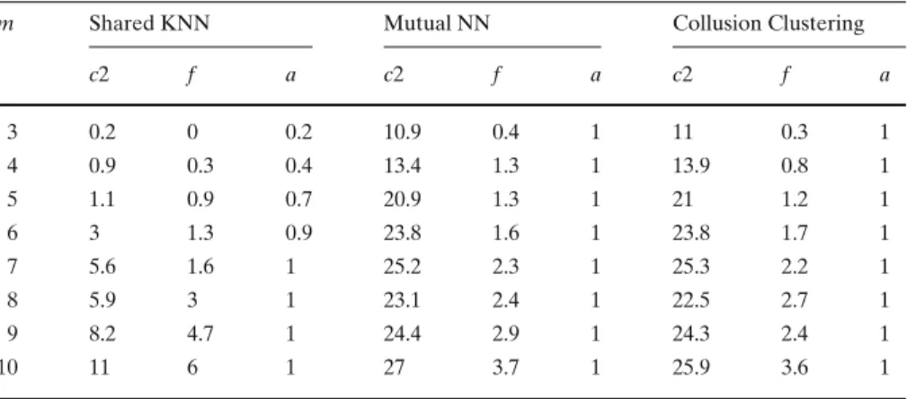
In the experiments to study the false alarm patterns for the algorithms, we generate the trading data as per the strategy reported in Sect.6.1. In each trial, we induce exactly one collusion set of size m in the trading dataset. We then compute the number of false alarms generated among the candidate collusion sets generated by each algorithm. We vary m from 3 to 10; for each value of m we repeat the experiment 10 times. Also, we do not consider candidate collusions sets of size 2, because such clusters can be found by querying or other simple techniques (we may not need the techniques in this paper).
Table 6 False alarms for the graph clustering algorithms
m Shared KNN Mutual NN Collusion Clustering
c2 f a c2 f a c2 f a
3 0.2 0 0.2 10.9 0.4 1 11 0.3 1
4 0.9 0.3 0.4 13.4 1.3 1 13.9 0.8 1
5 1.1 0.9 0.7 20.9 1.3 1 21 1.2 1
6 3 1.3 0.9 23.8 1.6 1 23.8 1.7 1
7 5.6 1.6 1 25.2 2.3 1 25.3 2.2 1
8 5.9 3 1 23.1 2.4 1 22.5 2.7 1
9 8.2 4.7 1 24.4 2.9 1 24.3 2.4 1
10 11 6 1 27 3.7 1 25.9 3.6 1
m: True collusion set size, c2: Average number of clusters of size 2, f : Average number of false
alarms (clusters of size>3 not containing the induced collusion set), a: Average number of times the true collusion set is detected
algorithm detected a total of 13 false alarms in 10 trials, giving an average of 1.3 false alarms per trial.
It is clear from Table6that the algorithms mutual_NN and collusion_cluste-ring show a smaller false alarm rate than shared_kNN algorithm. It can also be observed that the false alarm ratio f increases (for all three algorithms) as the true collusion set size m increases—a fact that is probably related to our data generation scheme.
7 Conclusions and further work
In this paper, we stated and formalized the important practical problem of detection of collusion among the traders in stock market. The problem of detecting colluding traders is important because many mal-practices in stock market trading—e.g., circular trading and price manipulation—use the modus
operandi of collusion. Investing public and institutions habitually lose vast sums
colluder. Each candidate collusion set can then be subjected to further in-depth analysis, to establish the occurrence of any collusion-based mal-practice.
We have used these algorithms on synthetic trading databases, where we created trading data based on different probability distributions and injected into them collusion sets of different sizes and characteristics. We have also tested these algorithms on real-life trading data.
We have found that all three algorithms are very efficient in handling large trading databases. We also found that all the three algorithms are very effective in detecting the candidate collusion sets. The most important advantage of these algorithms is that the users do not have to specify any background knowledge, training examples etc. (e.g., there is no need to specify what constitutes heavy trading). The algorithms are adaptive in the sense that they can be used without change for different securities having vastly different price and trading ranges. The reason is in the basic philosophy of these algorithms: which is to rank the vertices (or traders) rather than use numerical distance in terms of trading volume etc.
The novel idea proposed in this paper of combining results of different algorithms using Dempster–Shafer theory of evidence was also very useful and effective in focussing on more likely candidate collusion sets and thereby improving the accuracy of detection.
Our algorithms are oriented towards detecting relatively dense subgraphs of the stock flow graph. For example, purely circular trading among m traders will result in a circuit containing m edges, which is not a dense subgraph. Our algorithms will not always be able to detect such sparse subgraphs. The problem of detecting circuits is well-understood and there are well-known algorithms that can be used to detect circular trading. One possible strategy would be to detect circuits of size 3, check if they form a collusion, if yes, then remove the corresponding vertices from the stock flow graph, and then repeat the above steps for circuits of size 4, 5, 6 and so on. Our algorithms are oriented towards detecting collusions realized using much more random strategies.
As further work, we are investigating whether there are other and more effective ways of adapting the mutual NN and shared kNN graph clustering algorithms to the problem of collusion set detection. We are also investigating whether these techniques can be extended to detect occurrences of specific mal-practices such as price manipulation and circular trading. We are exploring whether classical statistical inference theory can be used to combine results of various experiments.
Appendix A. Example stock flow graph
We now give the data for the stock flow graph shown in Example 1. This graph has nine vertices and 50 edges. We associate two values with each edge label: volume and number of trades. Fig.1shows volume as the only edge label.
No. Seller Buyer Count Volume
1 1074 1054 62 15100
2 1042 1035 49 14300
3 1074 1035 54 13400
4 1042 1017 31 12400
5 1042 1037 39 11800
6 1057 1054 47 10800
7 1057 1037 14 9900
8 1049 1054 67 9600
9 1037 1054 55 9200
10 1074 1037 43 9200
11 1049 1042 63 9000
12 1042 1029 50 8900
13 1057 1017 21 8800
14 1074 1029 60 8500
15 1037 1029 38 8200
16 1049 1035 43 8200
17 1037 1017 66 7800
18 1074 1042 57 7500
19 1042 1054 42 7300
20 1057 1035 23 7000
21 1037 1074 29 6800
22 1074 1017 27 6700
23 1049 1037 40 5200
24 1057 1042 35 4700
25 1049 1017 18 4600
26 1037 1042 21 4400
27 1029 1054 32 3900
28 1049 1074 28 3600
29 1029 1037 25 3600
30 1057 1074 21 3200
31 1057 1029 26 3100
32 1029 1017 20 3000
33 1042 1074 19 2900
34 1029 1042 25 2600
No. Seller Buyer Count Volume
36 1049 1029 16 2100
37 1029 1074 15 1600
38 1074 1057 4 1500
39 1037 1035 3 700
40 1035 1054 4 600
41 1042 1057 4 600
42 1029 1057 3 500
43 1037 1057 1 200
44 1049 1057 2 200
45 1037 1049 2 200
46 1035 1029 2 200
47 1035 1042 1 100
48 1054 1029 1 100
49 1035 1017 1 100
References
Bapeswara Rao VV, Sankara Rao K (1985) Enumeration of Hamiltonian circuits in digraphs. Proc. IEEE 73:1524–1525
Gowda KC, Krishna G (1978) Agglomerative clustering using the concept of mutual nearest neigh-borhood. Pattern Recogn 10:105–112
Honkanen PA (1978) Circuit enumeration in an undirected graph. In: Proceedings of the 16th ACM southeast regional conference, pp 49–53
Jain AK, Duin RPW, Mao J (2000) Statistical pattern recognition: a review. IEEE Trans Pattern Anal Machine Intelligence 22(1):4–37
Jain AK, Murty MN, Flynn PJ (1999) Data clustering: a review. ACM Comput Surv 31(3):264–323 Jarvis RA, Patrick EA (1973) Clustering using a similarity measure based on shared nearest
neigh-bors. IEEE Trans Comput C-22(11):1025–1034
Le Hegarat-Mascle S, Richard D, Ottle C (2003) Multi-scale data fusion using Dempster–Shafer evidence theory. Integr Comput-Aid Eng 10:9–22
Palshikar GK, Bahulkar A (2000) Fuzzy temporal patterns for analysing stock market databases. In Proceedings of the international conference on advances in data management (COMAD-2000), Pune, India, Tata-McGraw Hill, pp 135–142
Palshikar GK, Apte MM (2005) Collusion set detection using graph clustering. In: Proceedings of the conference management of data (COMAD 2005b), Hyderabad, India, Computer Society of India, pp 101–111
Rich E, Knight D (1995) Artificial intelligence, 2/e. McGraw-Hill
Rubin F (1974) A search procedure for Hamilton paths and circuits. J ACM 21(4):576–580 SEBI Order against DSQ Holdings dated 10th December 2004. Order No. CO/109/ISD/12/2004.
http://www.sebi.gov.in
Shafer G (1976) A mathematical theory of evidence. Princeton University Press