Jena Research Papers in Business and Economics

Jena Research Papers in

Business and Economics

On the Part Inventory Model

Sequencing Problem: Complexity and

Beam Search Heuristic

Malte Fliedner, Nils Boysen, Armin Scholl

20/2007

Jenaer Schriften zur Wirtschaftswissenschaft

Working and Discussion Paper Series

School of Economics and Business Administration

Friedrich-Schiller-University Jena

ISSN 1864-3108

Prof. Dr. Hans-Walter Lorenz

h.w.lorenz@wiwi.uni-jena.de

On the Part Inventory Model Sequencing

Problem: Complexity and Beam Search

Heuristic

Malte Fliedner

_{, Nils Boysen}

_{, Armin Scholl}

a_{Universität Hamburg, Institut für Industrielles Management, Von-Melle-Park 5,}

D-20146 Hamburg, {fliedner,boysen}@econ.uni-hamburg.de

∗_{Corresponding author, phone +49 40 42838-4640.}

b_{Friedrich-Schiller-Universität Jena, Lehrstuhl für Betriebswirtschaftliche}

Entscheidungsanalyse, Carl-Zeiÿ-Straÿe 3, D-07743 Jena, a.scholl@wiwi.uni-jena.de

Abstract

In many industries mixed-model assembly systems are increasingly supplied out of third-party consignment stock. This novel trend gives rise to a new short-term sequencing problem which decides on the succession of models launched down the line and aims at minimizing the cost of in-process inven-tory held by the manufacturer. In this work, we investigate the mathematical structure of this part oriented mixed-model sequencing problem and prove that general instances of the problem are NP-hard in the strong sense. More-over, we develop a new Beam Search heuristic, which clearly outperforms existing solution procedures.

Keywords: Mixed-model assembly line; Sequencing; Consignment stock; Com-plexity proof; Beam Search

1 Introduction

The problem of optimally sequencing mixed-model assembly systems has been the subject of extensive research for more than four decades. Various exact and heuristic solution approaches have been developed for several well-known sequencing approaches like mixed-model sequencing (Thomopoulos, 1967; Tsai, 1995), car sequencing (Parello et al., 1986; Gagné et al., 2006) and level scheduling (Kubiak, 1993; Monden, 1998). An in-depth overview on model sequencing is provided by Boysen et al. (2007a). However, these

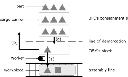
Figure 1: Schematic representation of the assembly line

traditional sequencing approaches are not sucient to cover the recent industry trend of consignment stocks:

Nowadays, Original Equipment Manufacturers (OEMs) more and more reorganize their material supply by relying on third-party consignment stock, which serves the assembly line with required material. In such a setting, the structure of the sequencing problem is much dierent from traditional model sequencing approaches. The material is supplied just-in-time by cargo carriers of a xed size from a consignment stock operated by a third-party logistics provider (3PL) adjacent to the line. In order to reduce the inventory held in possession by the OEM and to free valuable maneuvering space, a manufacturer in principle seeks to follow three simple policies, which are depicted in the schematic representation of the line in Figure 1:

(a) There is only a single cargo carrier per part in the possession of the OEM at a time from which a worker removes the required material part by part and assembles it into a workpiece which requires the respective product feature.

(b) Once the cargo carrier is emptied out by the worker, it is instantaneously removed from the station to free manoeuvering space. With regard to today's trend of de-creasing vertical integration and, thus, an ever inde-creasing number of parts to be assembled per station, the space at the assembly line is typically very scarce (see Klaemp, 2006; Boysen et al., 2007c).

(c) A new cargo carrier is issued as late as possible, that is, only if the current inventory of a part is zero and the respective part is required again by a model in the production sequence. Once a new cargo carrier crosses the line of demarcation, which typically separates the OEM's inventory from the consignment stock, the parts contained therein are automatically charged to the OEM by an online billing system.

Obviously, the model sequence heavily inuences the demand pattern of parts, so that model sequencing in a consignment stock setting aims at a demand pattern, which

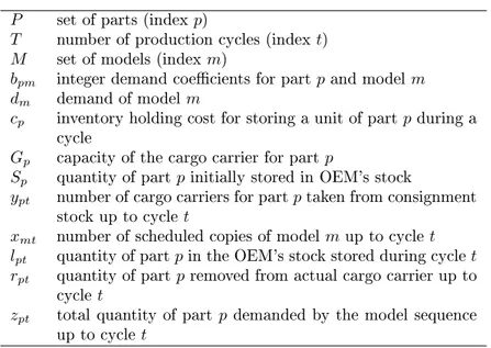
P set of parts (indexp)

T number of production cycles (indext) M set of models (indexm)

bpm integer demand coecients for partpand model m

dm demand of modelm

cp inventory holding cost for storing a unit of partpduring a

cycle

Gp capacity of the cargo carrier for partp

Sp quantity of partpinitially stored in OEM's stock

ypt number of cargo carriers for partptaken from consignment

stock up to cyclet

xmt number of scheduled copies of modelm up to cyclet

lpt quantity of partpin the OEM's stock stored during cyclet

rpt quantity of partpremoved from actual cargo carrier up to

cyclet

zpt total quantity of partp demanded by the model sequence

up to cyclet

Table 1: Notation

minimizes OEM's inventory costs. For this purpose, Boysen et al. (2007b) introduce the so called part inventory model sequencing problem (PIMSP), whose mathematical structure is presented in Section 2. The paper on hand broadens the work of Boysen et al. (2007b) in two directions. First (Section 3), we prove NP-hardness (in the strong sense) for general instances of PIMSP, which was only conjectured in the aforementioned paper. For the solution of PIMSP the preceding paper proposes an exact Bounded Dynamic Programming approach suited for small instances and two heuristic approaches (Goal Chasing and an Ant Colony approach) for instances of real world size. The paper on hand describes a heuristic Beam Search procedure (Sections 4.1 and 4.2), which clearly outperforms the existing procedures (Section 4.3). Finally, Section 5 concludes the paper.

2 Problem statement

In a consignment stock setting, model sequencing seeks to reduce the in-process inven-tory of parts, where the number of units lpt stored for part p during a cycle t can be

calculated by determining the total number ypt of issued cargo carriers of part p up to

cycle t and the cumulative part usage, which in turn depends on the total number of

scheduled model copies xmt over all types m assigned up to cycle t. With the help of

the notation summarized in Table 1, the PIMSP model contains of objective function (1) and constraints (2)-(8):

(PIMSP) MinimizeC(X, Y, L) =X p∈P (cp· T X t=1 lpt) (1) X m∈M xmt=t ∀t= 1, . . . , T (2) xmT =dm ∀m∈M (3) X m∈M xmt·bpm+lpt=ypt·Gp+Sp ∀p∈P;t= 1, . . . , T (4) 0≤xmt−xmt−1≤1 ∀m∈M;t= 2, . . . , T (5) 0≤ypt−ypt−1≤1 ∀p∈P;t= 2, . . . , T (6) ypt∈N0;lpt≥0 ∀p∈P;t= 1, . . . , T (7) xmt∈N0 ∀m∈M;t= 1, . . . , T (8)

The objective function (1) minimizes the total cost of inventory summing up the quan-titieslpt of all partspstored in all cyclesteach of which is weighted with the part-specic

inventory holding cost factor cp. Constraints (2) and (5) ensure that in each cyclet

ex-actly one model copy is produced, whereas equations (3) enforce that the demand dm

of each model m is met at the end of the planning horizon. The balance equations (4)

dene the quantitylpt stored per partpand cycletas the dierence between the overall

number of issued units (number of issued carriers ypt times carrier size Gp) plus initial

stock Sp and the cumulative consumption of the part by previously scheduled model

copies. Constraints (6) enforce the integer variables ypt to monotonically increase over

time.

3 Complexity of PIMSP

First, we will equivalently restate the original problem formulation of PIMSP to ease the formalization of the proof. Note that the number of part unitsrpt of partp which have

been removed from the actual cargo carrier at timetcan be calculated as follows: rpt=zpt+Gp−Sp− zpt+Gp−Sp Gp ·Gp = (zpt+Gp−Sp)mod Gp (9)

wherezpt denotes the total number of part units consumed by the model sequence up to

cyclet, i.e.,zpt=Pm∈Mxmt·bpmand 'mod' refers to the modulo division. If for a partp

initial stock is positive (Sp>0), it follows that there is a container forpat the beginning

of the planning horizon from which Gp−Sp units have already been removed. It holds

for alltsubsequent cycles within the horizon, that demandszptare additionally removed

from this and all further containers, each of which has size Gp. The modulo operation

thus yields the exact number of units removed from the current container int, as all prior

It follows that the actual number of stored units of part pat cyclet amounts to:

lpt = (Gp−rpt)mod Gp (10)

where the additional modulo division ensures that whenever no part unit is required from the next cargo carrier in cycle t(rpt= 0), its issuance is postponed, so that the current

inventory is zero.

Equations (9) and (10) can now be used to rewrite the model formulation as follows. MinimizeC(X) = T X t=1 X p∈P cp·(Gp−rpt)mod Gp (11) s.t. (2), (3), (5), (8) rpt= (zpt+Gp−Sp)mod Gp ∀p∈P;t= 1, . . . , T (12) zpt= X m∈M xmt·bpm ∀p∈P;t= 1, . . . , T (13)

The rewritten objective function (11) is still minimizing part inventory cost, merely the current inventory is now calculated dierently. Note, that rpt and zpt along with

restrictions (12) and (13) are introduced to ease the presentation, so that the only vari-ables really required in the restated formulation are the model assignments xmt. The

exact cycles in which new cargo carriers have to be issued (ypt) can be easily determined

for any given sequence by retrieving the actual cycles in which the number of removed units rpt just exceeds a new multiple of Gp for any partp.

3.2 Proof of NP-hardness for PIMSP

On the basis of the restated model formulation, we will proof NP-hardness for the general version of PIMSP. For this purpose we show how to transform instances of the 3-Partition Problem to PIMSP. The 3-Partition Problem is well known to be NP-hard in the strong sense (see Garey and Johnson, 1979) and can be summarized as follows.

3-Partition Problem: Given 3q positive integersat (t = 1, . . . ,3q) and a positive

in-teger B with B/4< at< B/2and P3t=1q at=qB, does there exist a partition of the set

{1,2, . . . ,3q} intoq sets {A1, A2, . . . , Aq}such thatP_t∈Aiat=B ∀i= 1, . . . , q ?

Transformation of 3-Partition to PIMSP: Consider an instance of PIMSP with two parts P ={1,2},T = 3q production cycles and M models in the setM ={1,2, . . . , M}

with demandsdm≥1 ∀m∈M andPm∈Mdm= 3q. Let inventory holding cost equal

one and initial inventories be zero (cp= 1, Sp = 0 forp= 1,2). The demand coecients

are

b1m=αm

b2m=B−αm

whereαm are positive integer values such thatB/4< αm < B/2and Pm∈Mαm·dm=

q·B and B is a positive integer.

Such a PIMSP instance can be derived in polynomial time from any instance of 3-Partition by grouping the set{1,2, . . . ,3q}intoM subsets{A∗

1, A∗2, . . . , A∗_M}, so that all

integers in such a subset are of the same size. That is, for each pair t, j ∈ A∗_m of each

subset m ∈ M, we have at = aj, while at 6= aj is true for all pairs t, j from dierent

subsetsA∗_m andA∗_nwithm6=n. The demand coecients for parts are then determined

via αm =at for all t∈A∗m, m∈ M and model demands are equal to dm =|A∗m| for all

m∈M.

Let the size of the two cargo carriers further be G1 = B and G2 = 2B. When

replacing rpt in (11) by the expression dened in (12) and considering the assumptions

oncp andSp, we can rewrite the objective function as follows (notice that the equivalence

(x+y)mod y ≡x mod y holds for integers x andy):

C = T X t=1 (B−z1tmod B)mod B+ T X t=1 [2B−z2tmod(2B)] mod(2B) = T X t=1

(B−z1tmod B)mod B+ [2B−z2tmod(2B)] mod(2B) (15)

We will now show that the instance of 3-Partition is a YES-instance if and only if there exists a solution to the respective PIMSP instance withC ≤3qB.

The rewritten objective function in (15) can be rearranged to C = P3q

t=1Ct with

Ct = (B−z1t mod B) mod B+ [2B−z2tmod(2B)] mod(2B). Due to the structure

of demand coecients it further holds that in any cyclet the cumulated requirement of

both parts together is a integer multiple ofB, i.e., we get

z1t+z2t=t·B for t= 1, . . . , T, (16)

which follows directly from the fact thatb1m+b2m =αm+B−αm=B for eachm∈M.

As further bpm > 0 is true for all p ∈ {1,2} and m ∈ M, part consumption is strictly

monotonically increasing:

zp,t+1 > zpt for p∈ {1,2} and t= 1, . . . , T−1 (17)

In dependence of the actual size ofz2t it can be shown that:

Ct=      0 , if z2tmod(2B) = 0 2B , if 0< z2tmod(2B)< B B , otherwise ∀t= 1, . . . , T (18)

In the following, these three cases are treated separately.

Case 1 (z2t mod (2B) = 0): Since z2t is a multiple of 2B it follows from (16) that

Ct=B mod B+ 2B mod(2B) = 0.

Case 2 (0 < z2t mod (2B) < B): Due to z2t mod (2B) < B, the following

equiva-lence holds: z2t mod (2B) ≡ z2t mod B. So, we get [2B−z2tmod(2B)] mod (2B) ≡

[2B−z2tmod B] mod (2B) ≡ 2B −z2t mod B. As at the same time the condition

of case 2 means that z2t is no multiple of B then due to (16) also z1t is no multiple of

B. From these preconditions it follows that Ct =B−z1t mod B+ 2B −z2t mod B =

3B−(z1tmod B+z2tmod B) = 3B−B = 2B.

Case 3 (B ≤ z2t mod (2B) < 2B): As z2t mod (2B) is bounded from above by 2B

this is the only case which remains to be investigated. Due to z2tmod(2B)≥B we get

z2tmod(2B)≡B+z2tmod B and(2B−B−z2tmod B)mod(2B)≡B−z2tmod B,

so that Ct = (B−z1t mod B) mod B+B−z2t mod B. Now, we distinguish between

two sub-cases:

(a) Ifz2tmod(2B) =Bthenz2tis a multiple ofBand due to (16), alsoz1tis a multiple

ofBso thatCt= (B−z1tmod B)mod B+B−z2tmod B =B mod B+B−0 =B.

(b) If z2t is not a multiple of B then due to (16) also z1t is not a multiple of B,

so that 0 < z1t mod B < B and Ct = B −z1t mod B +B −z2t mod B =

2B−(z1tmod B+z2tmod B) = 2B−B =B.

It can further be shown that any solution to such an instance will at least have q slots

where 0 < z2t mod (2B) < B and at maximum q slots where z2t mod (2B) = 0. The

latter follows directly from the fact thatz2T = 2qB and further (17) holds, so that only

q multiples of 2B can be met. The former is due to the fact that because of (14) all

demand coecient of part 2 are smaller than B. It follows that in the rst cycle and

subsequently in any cycle where z2t just exceeds a new multiple of 2B the dierence

between this multiple and z2i has to be smaller thanB so thatz2tmod(2B)< B. This

has to occurq times to reach z2T = 2qB. As further due to (18) the remainingq cycles

show at least a cost of B, it follows that CLB = 3qB is a lower bound on the objective

value.

We can transform the solution of any YES-instance of 3-Partition to a solution of PIMSP by simply arranging the setsAi in an arbitrary order and replacing each element

j ∈ Ai by the number of the model m to which it is assigned in the PIMSP-instance,

i.e., j ∈Am∗. Irrespective of the internal order within sets Ai, the restrictions imposed

on αm in (14) will lead to a production sequence wherez11< B/2 and B/2< z21 < B.

Applying (18) we get C1 = 2B. Furthermore, B/2 < z12 < B and thus B < z22 < 2B

so thatC2 =B. Finally, due to the denition of the partition we havez13=B, so that z23= 2B and C3 = 0, which sums up to inventory cost of 3B for the rst three cycles.

Note that after cycle 3 the total consumption of parts equals B and 2B for products 1

and 2, respectively, and the inventories are thus l13=l23= 0. As the same has to hold

for all subsequent triplets, the argumentation can be continued exactlyq times, resulting

Conversely, let us consider that a solution with an objective value C ≤3qB actually

exists. As was argued above, such an objective value can only be realized ifz2t becomes

a multiple of2B exactlyq times, which due to (16) means that z1t is also a multiple of

B for these slots. Now let us consider the part consumption at the beginning of such

a sequence. Because of (14) it holds that 0 < z12 < B and z14 < 2B, so that at the

same time due to (16) B < z22 < 2B and z24 > 2B. In other words, the cumulated

consumption of part 2 is always strictly lower than 2B up to slot 2, but strictly larger

than 2B after slot 4. If the consumption of part 2 is thus not equal to 2B at slot 3,

then due to (17) the rst multiple of2B cannot be met anymore and because of (18) the

objective value needs to increase by at least B, so that C ≥ (3q+ 1)B. It follows that

for a solution with C ≤ 3qB it has to hold that z23 = 2B and thus z13 = B. As this

means that l13 = l23 = 0, the argumentation can be continued in the same fashion for

all subsequent triplets, so thatz1,3·i=i·B for alli= 1, . . . , q, which immediately yields

the required partition.

The answer to the question of whether there exists a solution to an instance of 3-Partition is thus YES, if and only if there exists a solution with C ≤ 3qB for the

corresponding instance of PIMSP. As 3-Partition is NP-hard in the strong sense, so is the general version of PIMSP.

4 A novel Beam Search procedure

As the problem was shown to be NP-hard in the strong sense, heuristic solution ap-proaches are required to solve problem instances of real-world size. Beam Search is a truncated breadth-rst tree search heuristic and was rst applied to speech recognition systems by Lowerre (1976). Ow and Morton (1988) systematically study the performance of Beam Search compared to other well-known heuristics for two scheduling problems. Since then, Beam Search was utilized within multiple elds of application and many extensions have been developed, e.g., stochastic node choice (Wang and Lim, 2007) or hybridization with other meta-heuristics (Blum, 2005), so that Beam Search turns out to be a powerful meta-heuristic applicable to many real-world optimization problems. A review on these developments is provided by Sabuncuoglu et al. (2008).

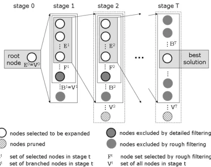
Like other breadth-rst search procedures, Beam Search relies on a tree representation of the solution space. Unlike a breadth-rst version of Branch&Bound, Beam Search restricts the number of nodes per stage to be further branched to a promising subset, which is determined by heuristic choices in a multi-stage ltering process. A schematic representation of Beam Search is depicted in Figure 2.

Starting with the root node of stage 0, all nodes (set V1) of stage 1 are constructed

and form the setB1 of branched nodes. Then, the multi-stage ltering process of Beam

Search starts to identify promising nodes of stage 1. First, a rough and computational inexpensive measure is applied within rough ltering. This measure, i.e. a priority rule or lower bound on the remaining path from the current node to the nal stage, assigns a priority value to each node within setB1, so that the rstF W nodes with regard to this

Figure 2: Schematic representation of Beam Search

priority value are chosen to form the set F1, where F W = |F1_{| is a control parameter}

called the ltered beam width. In the following step, so called detailed ltering is applied to further reduce node setF1_{to setE}1_{, which contains all nodes to be further branched in}

the succeeding stage. To choose the respective number of|E1_{|=BW nodes, whereBW}

is a control parameter called beam width, a more detailed and time-consuming inspection of nodes is applied. Typically, a more sophisticated lower bound procedure is utilized or even upper bound solutions are constructed by completing partial solutions (represented by the respective node) with a simple myopic priority rule based heuristic (e.g. Ow and Morton, 1988). Only the selected nodes contained in setE1 are branched to build the set B2 of branched nodes in stage 2, which is only a small subset of all possible nodes V2.

These steps are repeated until the nal stageT is reached, where the best solution out of

the setBT of constructed nodes is returned as the result of the Beam Search procedure.

4.2 A Beam Search procedure for PIMSP

To apply the general procedure of Beam Search in a specic domain the following three components must be specied with regard to the respective problem: (i) the graph structure and the measures for (ii) rough ltering as well as (iii) detailed ltering. In the following, we describe these specications for PIMSP:

Graph structure: The most obvious graph structure to be applied for sequencing problems like PIMSP is to let nodes of a stagetrepresent partial sequencesπ of models

up to sequence position t. We call the graph structure resulting from such an explicit

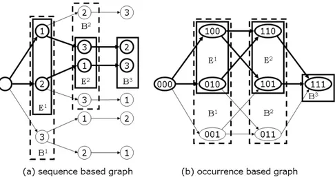
Figure 3: Alternative graph structures

most|M|nodes are to be branched, one for every model which still needs to be scheduled.

However, there exists a more compact graph representation of PIMSP, where a node rep-resents the number of occurrences of each single model up to staget. In such an implicit

enumeration scheme, a node of stage t represents multiple subsequences of models, i.e.

all subsequences (lled up to sequence positiont) which share the same number of model

occurrences irrespective of their exact order. Consequently, after branching into at most

|M|additional nodes from each node of a staget(like above) the resulting node setBt+1

is to be consolidated by deleting duplicate nodes with identical model occurrences. In such an occurrence based graph subsequences of models are represented by the dierent paths in the graph leading to a node. Figure 3 depicts both alternative graph structures for an example with 3 models with a demand of one copy each.

An occurrence based graph can be applied whenever the contribution to the objective value of a partial solution represented by a node at a current staget, exclusively depends

on the occurrence of models instead of their exact partial sequence. This is the case for PIMSP because inventory cost of cycletonly depends on the given initial inventories Sp

of part p, the cumulated production quantities Xtim, where Xtim denotes the number

of occurrences of model m of a node i in stage t and the size of the cargo carrier Gp.

The more compact occurrence based graph can be advantageous since the same node implicitly represents multiple subsequences, which are all evaluated in the process. In the sequence based graph each node merely represents a unique subsequence, so that with identical beam width BW less sequences are evaluated. This relationship becomes

obvious in the example of Figure 3, where ltered beam width F W and beam width BW are assumed to be 2. If the sequence based graph (a) is applied only 2 sequences

are evaluated, whereas the occurrence based graph (b) allows for an evaluation of 3 sequences. The evaluation of the advantage when applying the occurrence based graph is part of our computational study in Section 4.3.

of the set Bt into node setFt, we simply calculate the actual contribution of a partial

solution to the objective value. This contribution for an actual node(t, i)with cumulated

production quantities Xtim per modelm can be calculated as follows:

The produced quantities of all models up to cycle t in a state (t, i) directly determine

the cumulative demands Dtip for all partsp:

Dtip=

X

m∈M

Xtim·bpm ∀p∈P (19)

The inventories Itip of the parts p ∈P during a cycle t in state (t, i) are easily derived

by (20), because they are either units from initial stockSp not consumed by cumulated

demandDtip or residual units out of newly issued cargo carriers of sizeGp. The special

caseItip = 0arises when the carrier has been emptied at the beginning oftor was already

empty and no unit of phas been required in cycle t. Itip=      Sp−Dtip, if Sp ≥Dtip

0, else if (Dtip−Sp) mod Gp= 0

Gp−(Dtip−Sp) mod Gp, otherwise

∀p∈P (20)

Because the state(t, i)directly determines the quantities stored for each partp∈P, the

corresponding node can be assigned with a unique partial objective value ofRti equal to

the inventory holding cost at cyclet as follows: Rti=

X

p∈P

cp·Itip ∀t= 0, . . . , T;i∈Vt (21)

Our rough ltering selects the bestF W nodes with regard to the partial objective values Rti which form the set Ftand are further evaluated by detailed ltering.

Detailed ltering measure: Our detailed ltering procedure choosesBW(beam width)

nodes out of node set Ft. Only these BW remaining nodes are stored in setEt and are

considered for further branching. As a measure to prioritize single nodes (t, i) we

com-plete the partial solution represented by the respective node of stagetand determine an

upper bound solution. To do so, a simple myopic priority rule based approach is applied. At each remaining decision point τ = t+ 1, . . . , T only the set of possible alternatives P OSτ is relevant, which covers all modelsmwhose demand is not satised by the partial

solution of node (t, i) and preceding sequencing decisions between t+ 1and τ −1. Let

Dp(τ, m) =Pm0_∈MX_tim·b_pm0 +Pτ−1

t0_=t+1b_pπ

t0 +bpm denote the cumulative demand for

units of typep provided that modelm∈P OSτ is assigned to the current decision point

τ Then, for each model m ∈ P OSτ a priority value f(τ, m) has to be determined (see

f(τ, m) =X p∈P cp·      (Sp−Dp(τ, m)), if Sp ≥Dp(τ, m) 0, else if (Dp(τ, m)−Sp) modGp = 0 (Gp−(Dp(τ, m)−Sp))mod Gp, otherwise (22) Finally, with these priority values on hand, a greedy choice assigns the best model avail-able to the sequencing positionτ:

πτ =argminm∈P OSτ{f(τ, m)} (23)

Then,τ is incremented and choices are repeated until model vectorπ is completely lled.

In such a manner, all nodes of set Ft are completed to feasible solutions, and the best BW nodes are further branched in the next stage.

Finally, when the last stage is reached the best solution value is returned as the solution of our Beam Search approach for PIMSP.

4.3 Computational study

For our computational study we apply the 1458 test instances generated by Boysen et al. (2007b), which are downloadable under www.assembly-line-balancing.de. The over-all test bed is subdivided into smover-all (486 instances with a number of production cycles ranging between 10 and 20), medium (486 instances with 25-35 cycles) and large (486 instances with 100-300 cycles) instances. The methods described above have been imple-mented in Visual Basic.NET (Visual Studio 2003) and run on a Pentium IV, 1,800MHz PC, with 512MB of memory, which is the same conguration applied by Boysen et al. (2007b). Our computational study ought to answer the following three questions:

(i) Which parameter setting constitutes a reasonable compromise between solution quality and solution time for the Beam Search approach?

(ii) Does the Beam Search approach which relies on the occurrence based graph (BSo₎

outperform its counterpart relying on the sequence based graph (BSs)?

(iii) And nally, which performance does the Beam Search procedure show compared to the heuristic approaches provided by Boysen et al. (2007b)?

First, question (i) on a reasonable setting of control parameters F W (ltered beam

width) andBW (beam width) is investigated. For this purpose, we vary these parameters

in the following ranges: F W ∈ {10,15,20,25,30,35,40} and BW ∈ {5,10,15,20,25}.

For any feasible combination of control parameters (note that F W ≥BW has to hold)

we solve the set of small problem instances and relate the solution performance obtained to the respective control parameter values. These results are depicted in Figure 4.

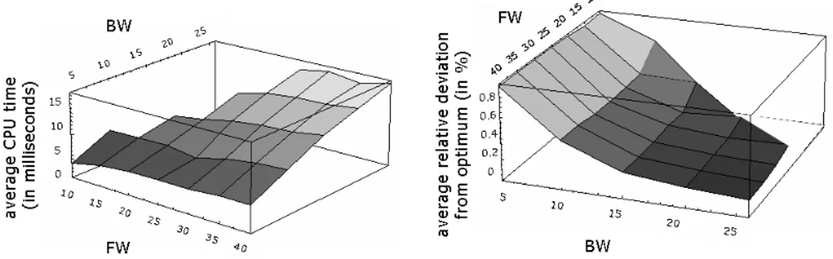
Figure 4: Solution time and quality in dependence of control parameters

Figure 4 displays that the solution time roughly increases in a linear manner if both

BW and F W rise. However, this increase is smaller with regard to a rising F W than BW, since the completion ofF W partial solutions by the myopic priority rule approach

during detailed ltering is computational inexpensive when compared to the more com-plex branching process ofBW nodes and the subsequent consolidation of duplicate nodes.

On the other hand, with rising F W andBW the solution quality increases. This result

is not astounding, because with increasing control parameter values a larger part of the complete solution graph is explored. In view of these results, we apply a parameter set-ting ofF W = 35andBW = 20for the following computational tests, which turns out to

be a reasonable choice to level the trade-o between solution quality and solution time. To answer questions (ii) and (iii), we solve all 1458 instances with our novel Beam Search approachesBSs basing on the sequence based graph and BSo (occurrence based

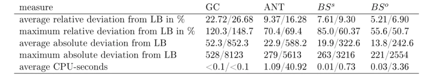
graph) and compare their results with the so-called Goal Chasing (GC) procedure, which is a simple myopic priority rule based heuristic, and the Ant Colony approach (ANT) provided by Boysen et al. (2007b). Table 2 displays the aggregated results over all small instances, where the results are compared in relation to optimal solution values. For the medium and large test instances these optimal solutions are unknown, so that Table 3 lists the aggregated results for these two instance sets compared to the results of a lower bound procedure (LB) introduced by Boysen et al. (2007b).

measure GC ANT BSs BSo

number of optimal solutions 89 323 340 435 average relative deviation from optimum in % 13.03 1.03 1.10 0.18 maximum relative deviation from optimum in % 123.08 11.2 30.0 5.42 average absolute deviation from optimum 17.3 1.9 1.59 0.36 maximum absolute deviation from optimum 246 44 33 22 average CPU-seconds <0.1 0.53 0.009 0.014

measure GC ANT BSs BSo

average relative deviation from LB in % 22.72/26.68 9.37/16.28 7.61/9.30 5.21/6.90 maximum relative deviation from LB in % 120.3/148.7 70.4/69.4 85.0/60.37 55.6/50.7 average absolute deviation from LB 52.3/852.3 22.9/588.2 19.9/322.6 13.8/242.6 maximum absolute deviation from LB 528/8123 279/5613 263/3216 221/2554 average CPU-seconds <0.1/<0.1 1.09/40.92 0.01/0.73 0.03/3.36

Legend: medium/big instances

Table 3: Results aggregated over all medium and large instances

These results reveal that BSo _{easily outperforms all other approaches by far. For}

instance,BSosolves 435 small instances to optimality with an average relative deviation

from the optimum of merely 0.18%. This is considerably better than the alternative Beam Search approach BSs _{(1.1%) and the heuristic approaches provided by Boysen et}

al. (2007b) (GC=13.03% and ANT=1.03%). Moreover, BSo is also considerably faster

than ANT. Analogously, BSo outperforms all other approaches when solving medium

and large test instances (see Table 3). Only with regard to the solution time BSs _is

slightly superior, which can be explained by the fact that the sequence based graph does not require a check for duplicate nodes. This consolidation step at each stage of the graph, which is inevitable for the occurrence based graph, slows down BSo_{. However,}

BSo is about 10 times faster than ANT and yields a considerably better solution quality.

5 Conclusion and Future Research

In this work, it was shown that general instances of PIMSP are NP-hard in the strong sense. Although from a practical point of view, average algorithmic performance is more conclusive with regard to the applicability of particular solution methods, the theoretic computational complexity of a problem provides valuable insights with regard to the choice of suited algorithms and constitutes a decisive step in understanding the prob-lem's structure. For a problem which is NP-hard in the strong sense, the existence of an exact algorithm with even pseudo-polynomial time complexity is highly unlikely, so that the development of specialized heuristic approaches seems meaningful in order to solve problem instances of real-world size. An appropriate Beam Search heuristic was addi-tionally developed. A comprehensive computational study showed that this approach clearly outperforms existing solution procedures.

Future research could investigate the question of whether special PIMSP-instances, consisting exclusively of zero-one demand coecients (bpm ∈ {0,1}), are also NP-hard

in the strong sense. Such a special structure of bills of material exists in some industrial cases (see Cakir and Inman, 1993; Boysen et al., 2007b), so that a respective proof would be a valuable contribution. Moreover other exact and heuristic algorithms could be developed to further enhance the solution performance.

References

[1] Blum C (2005) Beam-ACO Hybridizing ant colony optimization with beam ser-ach: An application to open shop scheduling, Computers & Operations Research 32: 15651591.

[2] Boysen N, Fliedner M, Scholl A (2007a) Sequencing mixed-model assembly lines: Survey, classication and model critique, European Journal of Operational Research (to appear).

[3] Boysen N, Fliedner M, Scholl A (2007b) Sequencing mixed-model assembly lines to minimize part inventory cost, OR Spectrum (to appear).

[4] Boysen N, Fliedner M, Scholl A (2007c) Level scheduling of mixed-model assembly lines under storage constraints, International Journal of Production Research (to appear).

[5] Cakir A, Inman RR (1993) Modied goal chasing for products with non-zero/one bills of material, International Journal of Production Research 31: 107115.

[6] Garey MR, Johnson DS (1979) Computers and intractability: A guide to the theory of NP-completeness, Freeman, New York.

[7] Lowerre BT (1976) The HARPY speech recognition system, Ph.D. thesis, Carnegie-Mellon University, U.S.A., April.

[8] Ow PS, Morton TE (1988) Filtered beam search in scheduling, International Journal of Production Research 26: 297307.

[9] Sabuncuoglu I, Gocgun Y, Erel E (2008) Backtracking and exchange of information: Methods to enhance a beam search algorithm for assembly line scheduling, European Journal of Operational Research 186: 915930.

[10] Wang F, Lim A (2007) A stochastic beam search for the berth allocation problem, Decision Support Systems 42: 21862196.