Experimental study of super-resolution using a compressive
sensing architecture
J. Christopher Flake
a,c, Gary Euliss
a, John B. Greer
b, Stephanie Shubert
b, Glenn Easley
a,
Kevin Gemp
a, Brian Baptista
b, Michael D. Stenner
a, Phil A. Sallee
ca
The MITRE Corporation, 7515 Colshire Drive, McLean, VA 22102;
b
National Geospatial-Intelligence Agency, 7500 Geoint Drive, Springfield, VA 22150;
cBooz-Allen-Hamilton, 8283 Greensboro Drive, McLean, VA 22102
ABSTRACT
An experimental investigation of super-resolution imaging from measurements of projections onto a random basis is presented. In particular, a laboratory imaging system was constructed following an architecture that has become familiar from the theory of compressive sensing. The system uses a digital micromirror array located at an intermediate image plane to introduce binary matrices that represent members of a basis set. The system model was developed from experimentally acquired calibration data which characterizes the system output corresponding to each individual mirror in the array. Images are reconstructed at a resolution limited by that of the micromirror array using the split Bregman approach to total-variation regularized optimization. System performance is evaluated qualitatively as a function of the size of the basis set, or equivalently, the number of snapshots applied in the reconstruction.
1. INTRODUCTION
The field of digital super-resolution has matured steadily over the last couple of decades, with a variety of algorithmic approaches proposed and demonstrated. Digital, or reconstruction-based super-resolution, usually refers to the reconstruction of a high-resolution image from multiple low-resolution images, where the resolution of the reconstructed image exceeds the detector-limited resolution of the imaging system. One of the earliest references on that topic is attributed to Tsai and Huang.1 Digital super-resolution relies on the presence of spatial aliasing in the low-resolution images.
Digital super-resolution is limited by the optical resolution of the imaging system used to acquire the low-resolution frames, but additional, more strict limitations on attainable low-resolution exist.2–4 The extent of limits on super-resolution remains to be fully explored. Despite these limits, commercialization of super-resolution has been occurring with a number products appearing on the market. The vast majority of prior research and development has occurred on the algorithmic side of the technology. Far fewer examples exist of cameras designed specifically with the capability of producing super-resolved images as an objective. These include cameras with image sensors that acquire multiple shots while the sensor physically shifts between shots.5, 6 As technology advances and the interest in imaging systems that take advantage of and even enable super-resolution grows, it becomes increasingly important to understand the limitations, how to mitigate those limitations, and how it all impacts choices in system design will become increasingly more important.
We present a compressive sensing image system designed for super-resolution: the Adjustable Resolution Compressive Sensing Imager (ARCSI). This ARCSI sensing model is designed for the field of remote sensing, where both the sensor and the target may be moving. Compressive Sensing (CS) is a methodology recently introduced that, among other goals, strives to make efficient use of sensor resources. Due to its novelty and potential, the interest in compressive sensing has steadily risen since the seminal papers of the mid-2000s.7, 8 CS presents entirely new ways to capture images that results in more efficient sampling and a corresponding
Send correspondence to John B. Greer
John B. Greer: E-mail: [email protected], Telephone: 571-557-2944
reduction in the amount of data required to capture the salient information in a signal. A recent application of CS to super-resolution is the simulations of Marcia and Willet.9 Their method modulates the Fourier transform of the signal while the ARCSI modulates purely in the spatial domain.
In traditional sensing, capturing a grayscale image withN pixels requiresN measurements. For the sake of conversation, suppose thoseN measurements corresponded to N bytes of data. In order to store or transmit that same image, we typically compress it to a fractional number of bytesK << N with minimal, or even no, visible loss. This suggests that traditional imaging is non-optimal, since we had to collectN bytes of data to getK bytes of information. Ideally, we would collect theK essential measurements at the start, thus reducing sensing costs in the form of energy, equipment, and time. Of course, compression relies on the fact that we have gathered the full image and can then decompose that image into a basis in which it is sparse (e.g. a wavelet or a cosine basis). The surprising result of CS is that we do not need to collect the fullN bytes of data. CS theory shows7, 8 that while we cannot get away with only K measurements, for certain appropriate measurements, we only need a number of measurements that grow asO Klog NK
.In addition, we can do this without choosing ahead of time the basis that best represents the image.
In order to improve upon traditional sensing, CS requires a restricted set of measurements that correspond to matrices satisfying what is called the Restricted Isometry Property (RIP).7 Determining whether a given sensing matrix satisfies RIP is known to be an NP-complete problem.10 However, it is also known that Bernoulli and Gaussian matrices make up a useful collection of sampling matrices that have a very high probability of satisfying RIP.
Rice’s single pixel camera11 demonstrates one of the first applications of CS theory to gray-scale imaging. Benefits of this architecture include a combination of lower cost, higher information efficiency and flexibility in sensor application. The camera uses a single photodetector and a Digital Mirror Device (DMD) to implement random matrices that have been shown to meet CS requirements. By selecting random patterns with the mirrors that block half incoming light, each measurement by the detector gathers the total light from half of the scene. Rapidly changing the pattern with each measurement, at roughly twelve thousand times per second, allows gathering sufficient data to reconstruct the image plane. The camera is an impressive demonstration of how CS might be applied to practical sensing devices, but it is not well suited to remote sensing. The sensor trades number of detector elements for collection time, and while CS allows the sensor to get away with far fewer measurements than traditional sensors, it still requires enough measurements that would make it impractical for a moving platform imaging objects that might be moving themselves.
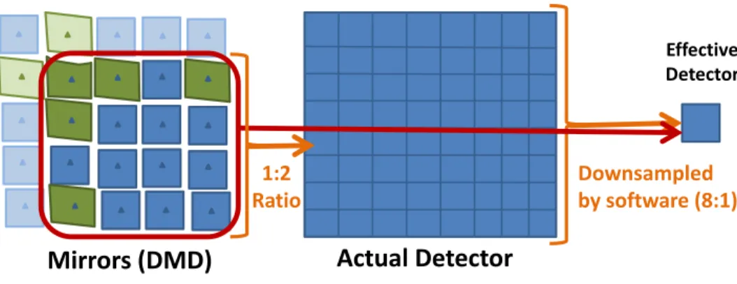
Inspired by the single pixel camera, we apply Bernoulli sensing matrices and DMDs to a more traditional sensing architecture in an attempt to boost the imaging system’s resolution. Our goal is to use the optimal sensing of CS to boost the imaging system’s resolution. The new system, ARCSI, has a detector array that does not fully resolve the smallest length scales captured by its optics, and a DMD, with a higher resolution than the detector. We increase image resolution by taking multiple low-resolution snapshots, each with a unique random binary pattern. We then solve an inverse problem to reconstruct an image with a number of pixels equivalent to number of mirrors in the DMD, see Fig. 2. Although our device uses a DMD, a set of fixed coded apertures could be used, and indeed would be more practical for imaging with just a couple of snapshots. A useful property of the ARCSI is that any single snapshot can stand-alone as a low-resolution image. Acquiring additional information then allows the user to enhance resolution as needed.
The ARCSI sensor has the potential to be useful within the general constraints of remote sensing, and in the process has expanded our understanding of how the physical realities of implementing a sensor interfere with achieving many of the desired theoretical assumptions. In the next section we describe the experimental setup and computation of the sensor forward model. Next we briefly outline the reconstruction method for inverting the compressive sensing operator. Experimental results are provided as a qualitative assessment of the super-resolution performance, followed by what we have concluded from the research.
2. SENSOR SETUP AND MODEL
The basic design of ARCSI has a lot in common with previous demonstrations of compressed sensing, and in particular, the seminal work of Duarte et al.11 and Marcia and Willet.9 The primary difference is that ARCSI
uses a full CCD array, as opposed to an individual detector or a small set of individual detectors and modulates exclusively in the spatial domain. As a result, a single snapshot with ARCSI gives a recognizable image. The DMD is only used to increase resolution.
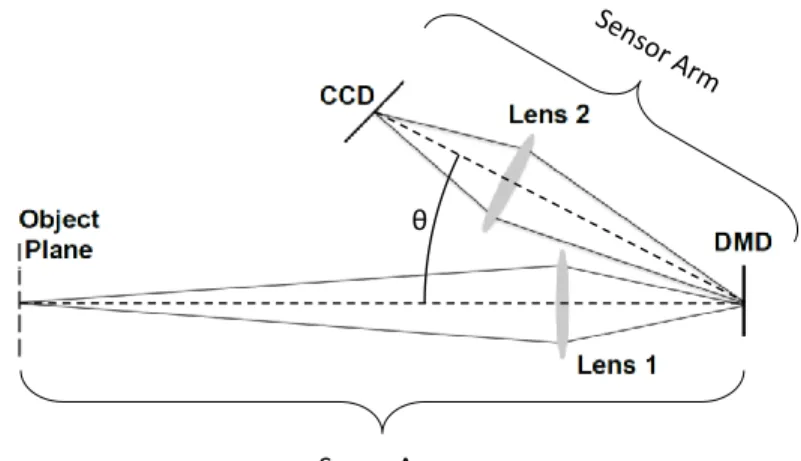
Fig. 1 illustrates the 2 imaging arms of the ARCSI system configuration. In the scene arm, a field lens (Lens 1 in the figure) is used to form an intermediate image of the object plane, or scene, onto the DMD. The sensor arm then relays the intermediate image by using an eye lens (Lens 2) to image the DMD onto a CCD sensor. Specifications for the DMD are summarized on the manufacturer’s website.12 ARCSI selected a combination of vendors’ stock lenses using optical modeling. The scale of the setup was constrained to fit on a 60×40 optical table.
Scene Arm θ
Figure 1: Diagram illustrating the experimental setup used to acquire ARCSI data. Lens 1 forms an image of the object plane on the DMD which is spatially coded with a binary pattern. Lens 2 then forms an image of the object plane multiplied by the binary pattern. Note that the figure is not to scale.
As Fig. 1 illustrates, in the sensor arm the DMD is tilted with respect to the optical axis. This is required in order to focus the intermediate image on the DMD across the entire field of the CCD. The angle of the optical axis for the sensor arm with respect to that of the scene arm is fixed by the angle (θin the figure) at which the DMD micro-mirrors tilt when in the “on-state.” The eye lens is positioned normal to the optical axis for the sensor arm. The angle of the CCD then is set according to the Scheimpflug principle which directs that the focus, lens and object planes (which in this case is the plane of the DMD) will simultaneously intersect on a line.13 In addition to this tilt, the DMD is also rotated 45o around the normal to it’s surface. This rotation is introduced so that the micromirrors, which tilt about their diagonals, will deflect rays incident from the object in the plane of the optical table. The CCD is also rotated about it’s normal to maintain the same geometry as the DMD. Custom mounts were designed and fabricated for the DMD and the camera to establish this configuration.
An Andor Luca-R electron multiplication CCD (EMCCD) camera was used to acquire the data. EMCCDs offer the advantage that gain can be applied to the data prior to readout, thus avoiding amplification of read noise. Low-noise sensor options are appealing because reconstruction algorithms used in compressive sensing, including the one described in Sect. 3, tend to degrade when noise is introduced in the data. Specifications for the Luca-R are given in Table (1). The quantum efficiency of the device is well over 50% for most of the visible spectrum. The camera contains a thermoelectric cooler and operates at -20 oC to reduce thermal noise. The CCD and Lens 2 were positioned to achieve a magnification corresponding to approximately one DMD mirror to each CCD pixel. As will be discussed below, the data is down sampled by binning 4×4 pixels to simulate a low resolution sensor, see Fig. 2. This results in approximately 4×4 micromirrors to each effective low-resolution CCD pixel. Down sampling in software is useful because it allows us to study the effects of various ratios of
mirrors to detector elements in a laboratory setting. Because of the distortion introduced by the tilted planes of the CCD and DMD, it was not possible to attain that magnification across the field. It was also not feasible to establish exact registration between micromirrors and pixels. Binary patterns are written to the DMD through a computer interface. Given the setup shown in Fig.1, the image incident on the CCD is then the product between the scene image and the pattern displayed on the DMD.
Effective Detector
Mirrors (DMD)
Actual Detector
Downsampled
by software (8:1)
1:2
Ratio
Figure 2: Sensor schematic showing the relative magnification between DMD and detector plane (1 : 2) and then the software down-sampling operation effectively making the compression ratio from DMD to effective detector as 16 : 1. This configuration allows the study of various ratios of mirrors to detector elements.
Active Pixels 1004×1002 Pixel Size (µm) 8×8 Image area (mm) 8×8 Active area pixel well depth 30000 Gain register pixel well depth 80000 Max readout rate (MHz) 13.5
Frame rate (per second) 12.4
Read Noise (e−) <1 to 18 @ 13.5 MHz Table 1: Andor Luca R specifications.
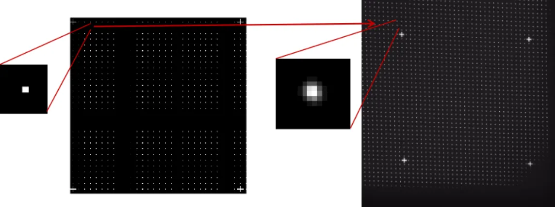
To successfully perform super-resolution, we need an accurate sensor forward model mapping high resolution images to ARCSI measurements. For our purposes, we only need to model the DMD to detector arm of the sensor, resulting in reconstructions with a number of pixels determined by the size of the DMD. Accurately modeling the performance of ARCSI requires measuring the system response to each individual mirror on the DMD. We do this by imaging flats with every tenth mirror turned on along both axes. We shift the pattern of activated mirrors through 100 images to account for all mirrors. A single image from this calibration process is illustrated in Fig. 3.
As with any CCD-based detector, before any processing, all calibration data requires correction to remove any detector artifacts.14 We remove scattered light and dark current by subtracting a frame collected with the light source on and setting all of the mirrors to the off state. This frame is collected using the same exposure times as the calibration data. Finally, we apply a multiplicative flat field correction for the differences in pixel-to-pixel response, gain variation across the detector, and field illumination. These correction frames are all median combinations of many frames of each type which we measure at start of a collection run.
Figure 3: One frame of a typical ARCSI calibration. The left image is the input to the DMD while the right image is the response on the detector. The zoom-in shows the size of the psf. Matching the pixel on the left with a patch on the right allows us to build a precise linear model for the camera.
and the detector that is built from the calibration data, a masking operator Λ determined by the pattern of activated DMD mirrors, and a downsampling operatorD:
A=DΛO. (1)
Given a DMD stateB, whereBis a binary array, we place the values ofB onto the diagonal of a very large sparse array Λ. Finally, we apply a down-sampling operator,D, which takes each group of 4×4 pixels on the detector and produces a single average of those 16 pixels.
The sensor matrix for multiple snapshots is created by tiling single-snapshot matrices for a collection of DMD patterns,B1,B2, . . . ,BL, and corresponding diagonal matrices Λ1,Λ2, . . . ,ΛL:
A= DΛ1O DΛ2O .. . DΛLO (2)
The data acquired consists of a set of low-resolution measurements from random inner-products on a local level. The masks are drawn from a uniform random distribution with the constraint that each 4×4 block has precisely 8 mirrors turned on and 8 turned off.
3. RECONSTRUCTION
Underdetermined inverse problems have gained quite a bit of interest in the last decade and are increasingly available to users as convenient software packages.15–17 The goal of this project explicitly involves demonstrat-ing a realistic implementation of a CS-like camera for flexible remote sensdemonstrat-ing. We therefore do not concentrate on optimizing the reconstruction method, parameter space, or reconstruction time. There is far more research
that could be conducted to determine effective reconstructions for the ARCSI, including learned-dictionary regularization18, 19or Bayesian methods.20 The most effective reconstruction methods used total-variation regu-larization.21, 22 Promising reconstructions were also found by balancing the total-variation against a smoothing wavelet.
3.1 Split Bregman: total variation and wavelet regularization
LetAbe the ARCSI linear sensor model. Suppose that u∈RN is a high-resolution image withN pixels. Then
A maps u onto a sample, y = Au. The goal is to take A which is given (or in our case measured from the sensor directly) and the sampley, which is a collection ofM low-resolution measurements, and come up with the correct high-resolution imageu. Since M < N the inverse problem is underdetermined and therefore we need to regularize the optimization problem to select one answer from the infinite dimensional null-space ofA. We settled on the following problem statement:
u∗= arg min u ||Au−y|| 2 2+λ1 W−1u 1+λ2||∇u||1, (3)
whereWis a wavelet transform with coefficientsα=W−1u.
Equation (3) with λ1 = 0 tends to produce reconstructions with sharp contrasting edges while smoothing regions of low contrast. Thought to be nearly optimal for cartoon-like images, the results can appear like an oil painting if the sampling operator is severly undersampled. Equation (3) withλ1 ≥ 0, λ2 > 0 allows more smooth structures to be reconstructed. For most imagery that we investigated, Equation (3) produced better reconstructions withλ1= 0 while a small percentage of imagery responded well to the wavelet regularization by allowingλ1>0. In either case, we used a split-Bregman implementation22to quickly solve the inverse problems. This involved using few outer iterations and many inner iterations.
4. RESULTS
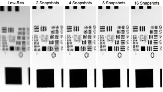
In the following section, we present a series of results from data acquired and processed during the experiments described above. These results qualitatively demonstrate super-resolved images from groups of detector-limited images projected onto a random binary basis set. In each collection of results, we provide examples of images reconstructed using as few as two and as many as 16 snapshots to illustrate the tradeoff between image quality and the amount of data required to reconstruct the associated images. The first of these results is presented in Fig. 4 and corresponds to images from a standard resolution target. The image on the far left and labeled low-res is a single image acquired with all of the DMD mirrors switched to the on position, and then down sampled by binning pixels on the CCD in 4×4 blocks. We preserve subsets of masks, so the reconstruction using 16 snapshots has the same 8 masks from the 8 snapshot reconstruction and 8 additional snapshots. The same relationship exists between 8 and 4 snapshot reconstructions.
The smallest set of bars have roughly 3 times the spatial frequency as the largest full set of bars. This visually confirms the increase of resolution to roughly 3×between the low-resolution image and the 16 snapshot reconstruction. An argument can be made that the total variation method of image reconstruction can artificially sharpen a binary image with well defined edges such as the images represented in Fig. 4. To address that concern, two additional examples are provided in Fig. 5 and Fig. 6. In Fig. 5, the object corresponds to a small region of a dollar bill with it’s associated fine spatial details. Much of that detail is lost in the single low-resolution image represented on the left. As we move from left to right in the figure and additional snapshots are included in the reconstruction, qualitative improvements can be seen in the images. Note that these images have been processed using the same method applied in Fig. 4. To reiterate, these improvements come at the expense of additional data collection, storage, and processing.
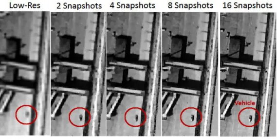
The final example we present is shown in Fig. 6 in which the object is an overhead photograph of an airport. This example demonstrates how the level of object discrimination is increased when additional snapshots are included in the reconstruction. For illustration, we have highlighted a vehicle in the lower part of the image with a circle. In the low-resolution representation, the vehicle is detectable but otherwise unrecognizable at any higher level of discrimination. As more snapshots are added to the reconstruction, spatial details begin to emerge until the object is recognizable as a vehicle. Other evidence of increased resolution can be found in the images as well.
Figure 4: An example of images reconstructed from 2 - 16 snapshots using the approach described in Sect. 2. The image on the left represents a single down sampled acquired with all mirrors on and then binning the detector.
Figure 5: An example using a grayscale object with fine spatial details. Qualitative improvements in the image resolution are visible as additional snapshots are included in the reconstructions.
Figure 6: In this example, the object is an overhead photograph of the Zurich airport (terminal B) taken with Quickbird sensor via Google Earth. The ability to discriminate the vehicle (highlighted in the circle) improves as the number of snapshots increases.
5. CONCLUSIONS
In this paper, we have experimentally demonstrated image super-resolution from a tabletop imaging sensor inspired by previous demonstrations in compressive sensing. In particular, the sensor described here acquires images projected onto a subset of a random binary basis, but performs that acquisition on a CCD as opposed to a single detector or small collection of detectors. The approach presented, including the method chosen for image reconstruction, was motivated largely by remote sensing as an application and the interest in an alternative super-resolution solution suitable for that application.
Three sets of reconstructed images were presented corresponding to data acquired from three different subject matters representing a range of characteristics from simple binary to grayscale with varying levels of spatial detail. In each of these examples, super-resolution was successfully demonstrated to varying degrees. Also provided by the results is a qualitative study of how the resolution of the reconstructed images improves with the number of projections used in the reconstruction. Given that more snapshots equate to the collection of more data, the study highlights the fundamental tradeoff between image resolution and data volume. By furthermore acknowledging a relationship between resolution and information, the tradeoff between resolution and data can be translated to a tradeoff between information and data. And while a resolution/information gain is evident in the results presented, we cannot conclude from these results alone whether or not there is any information efficiency advantage to this approach.
REFERENCES
[1] Tsai, R. Y. and Huang, T. S., “Multi-frame image restoration and registration,” in [Advances in Computer Vision and Image Processing],1, 317–339, JAI Press Inc., Greenwich, CT (1984).
[2] Baker, S. and Kanade, T., “Limits on super-resolution and how to break them,” IEEE Transactions on Pattern Analysis and Machine Intelligence24(9), 1167–1183 (2002).
[3] Lin, Z. and Shum, H.-Y., “Fundamental limits of reconstruction-based superresolution algorithms under local translation,”IEEE Transactions on Pattern Analysis and Machine Intelligence26(1), 83–97 (2004). [4] Farsiu, S., Elad, M., and Milanfar, P., “Advances and challenges in super-resolution,”International Journal
of Imaging Systems and Technology14, 47–57 (2004).
[5] Ben-Ezra, M., Zomet, A., and Nayar, S., “Jitter Camera: High Resolution Video from a Low Resolution Detector,” in [IEEE Conference on Computer Vision and Pattern Recognition (CVPR)],II, 135–142 (Jun 2004).
[6] http://www.hasselblad.com/products/h-system/h5d-multi-shot.aspx (2014). The Hasselblad H5D-200MS camera uses a sensor that shifts between each of 4 or 6 shots.
[7] Candes, E. J., Romberg, J., and Tao, T., “Robust uncertainty principles: Exact signal reconstruction from highly incomplete frequency information,”IEEE Trans. Inform. Theory52, 489–509 (February 2006). [8] Donoho, D., “Compressed sensing,”Information Theory, IEEE Transactions on52, 1289–1306 (April 2006). [9] Marcia, R. and Willett, R., “Compressive coded aperture superresolution image reconstruction,” in [ Acous-tics, Speech and Signal Processing, 2008. ICASSP 2008. IEEE International Conference on], 833–836 (March 2008).
[10] Bandeira, A., Dobriban, E., Mixon, D., and Sawin, W., “Certifying the restricted isometry property is hard,”Information Theory, IEEE Transactions on59, 3448–3450 (June 2013).
[11] Duarte, M., Davenport, M., Takhar, D., Laska, J., Sun, T., Kelly, K., and Baraniuk, R., “Single-pixel imaging via compressive sampling,”Signal Processing Magazine, IEEE25(2), 83–91 (2008).
[12] https: //www.dlinnovations.com (2014). DLI offers the DMD from Texas Instruments integrated into a developers kit.
[13] Scheimpflug, T., “Improved method and apparatus for the systematic alteration or distortion of plane pictures and images by means of lenses and mirrors for photography and for other purposes.” GB Patent No. 1196 (1904).
[14] Howell, S. B., [Handbook of CCD Astronomy], Cambridge University Press (2006).
[15] Li, C., Yin, W., Jiang, H., and Zhang, Y., “An efficient augmented lagrangian method with applications to total variation minimization,”Computational Optimization and Applications56(3), 507–530 (2013). [16] Bioucas-Dias, J. M. and Figueiredo, M. A. T., “A new twist: Two-step iterative shrinkage/thresholding
algorithms for image restoration,” (2007).
[17] Figueiredo, M. A. T., Nowak, R., and Wright, S., “Gradient projection for sparse reconstruction: Application to compressed sensing and other inverse problems,”Selected Topics in Signal Processing, IEEE Journal of1, 586–597 (Dec 2007).
[18] Soni, A. and Haupt, J., “Learning sparse representations for adaptive compressive sensing,” in [Acoustics, Speech and Signal Processing (ICASSP), 2012 IEEE International Conference on], 2097–2100 (March 2012). [19] Mairal, J., Sapiro, G., and Elad, M., “Learning multiscale sparse representations for image and video
restoration,” tech. rep. (2007).
[20] Ji, S., Xue, Y., and Carin, L., “Bayesian compressive sensing,” (2007).
[21] Rudin, L. I., Osher, S., and Fatemi, E., “Nonlinear total variation based noise removal algorithms,”Physica D60, 259–268 (1992).
[22] Goldstein, T. and Osher, S., “The split bregman method for l1-regularized problems,”SIAM J. Img. Sci.2, 323–343 (April 2009).