PROFILE OF
LEVERAGE AND
INVERSE ETF
S
We derive a model for the performance and sharpe-ratio of leveraged and inverse index funds which follow a dynamic leveraged trading strategy, i.e. they are re-balanced on a daily basis to ensure a constant degree of leverage with respect to the underlying. We show that the performance behaviour shows a trade-off between exploiting higher growth rates due to leverage and performance losses due to the volatility of the underlying. Further, we assess the importance of transaction costs for leveraged and short ETFs. As a consequence, we find that there is an optimal degree of leverage which is supported by numerical simulations.
INTRODUCTION
Leveraged investment products have become a widely used asset class in both the derivative market and the ETF market (cf EDHEC 2009). With the recent financial turmoil ETFs have become increasingly popular in comparison with derivative structured products, in particular long and short leveraged ETFs, which offer a different type of leverage strategy compared with certificates. In simple words, leveraged certificates such as mini-futures typically offer a leverage effect in the form of a constant Delta with respect to the underlying and consequently a time varying leverage factor when the price of the underlying changes. In contrast to certificates, leveraged funds follow a dynamic leverage trading strategy to achieve a constant leverage factor but a time varying Delta exposure with respect to the underlying by a daily re-balancing of the investment portfolio.
At issuance, both strategies have in common that a certain leverage L is achieved by borrowing (L-1) times the investment amount to be able to invest L times the investment amount into the underlying asset and hence both strategies incur refinancing costs. However, while the replicating investment portfolio of a leveraged certificate is essentially constant in time (refinancing costs are continuously accrued and reflected in the portfolio value), leveraged ETFs are rebalanced every day to ensure a constant leverage L of the fund, i.e. the ratio between the investment amount in the underlying and the size of the refinancing loan is kept at a level of L / L-1 on a daily basis. The difference between the two strategies is summarized. in Table 1:
Leveraged certificate Leveraged fund
Stylised pay-off C = C0 + L(S-S0) F = F0 (S/S0)L Delta = dC/dS L = L F0 (S/S0)L-1 / S0 Leverage = / C * S = L * S / C = / F * S L
Table 1: The stylised pay-off of a leveraged certificate with constant Delta versus the stylised pay-off of a leveraged fund strategy with constant leverage on the same underlying S.
Leveraged funds and short funds are typically issued in the form of an index fund tracking a leveraged equity index, which exist for all major blue-chip equity indices (e.g. leveraged versions of the EuroSTOXX 50, CAC40, DAX, DowJones, S&P500 etc.) and for many sector specific indices (pharmaceuticals, oil & gas etc.). On the long side, by far the most popular strategy is a leverage of two, but most index providers have also issued leverage three or even leverage four versions, at least on their respective blue-chip indices. On the short side, the single short (i.e. leverage one) strategy is by far the most commonly used, but most index providers have added double short indices which use a leverage of two.
The advantage of the dynamic leveraged index fund strategy is the fact that in falling markets the Delta exposure is automatically reduced and hence the product value always stays positive, whereas the value of a certificate can reach zero and the certificate ceases to exist. Analogously, in bullish markets the leveraged fund gears up the portfolio on a daily basis and hence profits more from the rising underlying price than the certificate. On the other hand, the re-balancing of the portfolio of a leveraged fund creates an adverse influence of volatility on the performance, as the following example in Table 2 illustrates:
Day Underlying Change Certificate Change Fund Change
1 100 - 100 - 100 -
2 80 - 20% 60 - 40% 60 - 40%
3 100 +25% 100 + 67% 90 + 50%
Table 2: Example of an underlying asset S and a certificate with Delta=2 and a fund with leverage=2 thereon. The underlying returns to the initial value of 100 after two trading days, the same is true for the certificate, whereas the leveraged trading strategy suffers a loss, which increases in the volatility of the underlying and the degree of leverage as we will show below.
In the example in table 2, the volatile behaviour of the underlying has not changed the value of the underlying, but incurred a loss on the dynamic leveraged strategy, which is proportional to the variance of the underlying as we will see below.
A similar statement holds for short strategies as we indicate in the following table, comparing a short certificate to a short fund over three consecutive trading days:
Day Underlying Change Short Certificate Change Short Fund Change
1 100 - 100 - 100 -
2 80 - 20% 120 +20% 120 + 20%
3 100 +25% 100 -16.67% 90 - 25%
Table 3: Example of an underlying asset S and a short certificate and a short fund (both with leverage one) thereon. The underlying returns to the initial value of 100 after two trading days, the same is true for the short certificate, whereas the leveraged trading strategy suffers a loss, which increases in the volatility of the underlying and the degree of leverage as we will show below.
Consequently, while the long-run performance of the leveraged certificate is L times the underlying performance less refinancing costs, the performance of the leveraged ETFs is more complex and depends on three parameters:
1. The growth rate of the underlying - the higher the more attractive leverage becomes 2.The refinancing rate r – the higher the less attractive leverage is.
3.The volatility of the underlying – the higher the less attractive leverage becomes.
Points 1 and 2 are also determinants for the performance of a leveraged certificate. However, points three is specific for leveraged funds and is due to the daily rebalancing of the portfolio.
Although leveraged and inverse ETFs have become standard products in the financial industry, recent studies (cf Cheng 2009, Despande 2009 and Lu 2009) have pointed out that the performance
characteristics of these strategies is fairly complex. In particular, the long term performance of these funds is path-dependent with respect to the underlying and is strongly influenced by the volatility of the
underlying. Consequently, the long term performance is not simple L times the performance of the underlying asset, but can be substantially higher or lower, depending on the behaviour of the underlying. As a consequence, the authors point out that these products are often misunderstood by market participants, in particular regarding the degree of market risk implied by these strategies.
The purpose of this paper is to develop a very general model for the long-term performance of a dynamic leveraged and inverse fund strategy and to analyze its risk-return profile in detail in order to provide a detailed insight for investors into the behaviour of these financial products.
MODEL DESCRIPTION FOR LONG LEVERAGE
We assume an underlying equity index S of the leveraged fund that follows a stochastic process, i.e. with the growth rate u and volatility we have
dS
t
S
t(
udt
dW
t)
1Where Wt denotes a standard Wiener process. Consequently,
ut
S
S
E
W
t
u
S
S
t t texp
2
exp
02
0
2
As funds typically track the total return versions of equity indices where dividends are assumingly re-invested, we can neglect the role of dividends and assume S to be the total return version of an equity index.
The process for a leveraged fund F on the underlying asset S with leverage factor L reads (cf NYSE Euronext 2008, STOXX 2010)
dF
t
F
tL
(
udt
dW
t)
F
t(
L
1
)
rdt
3
In practice, the term dF refers to the daily change of the funds value, where the fund manager borrows (L-1) times the value of the fund, incurring refinancing costs at the rate r, to invest L times the net asset value of the fund into the underlying S. Due to the daily rebalancing, the leverage is kept constant at the level L. At a first glance one could assume that the process (3) results in a fund value which is the L-th power of the underlying value (2) less financing costs, i.e. one can make the following approach for the fund value
L
rt
S
S
F
F
L t at
exp
(
1
)
0
0
4
However, applying Ito’s Lemma (cf Baxter 1996) we observe that the differential equation for (4) reads:
dt
L
L
F
rdt
L
F
dW
udt
L
F
dF
ta ta t ta ta(
1
)
22
1
)
1
(
)
(
5 Which does not coincide with the investment strategy (3). Comparing equations (5) and (3) we conclude that the actual value of the leveraged fund F includes an additional term representing the afore-mentioned volatility related performance impact and hence instead of equation (4) the value of the fund reads:
L
rt
L
L
t
S
S
F
F
L t t 2 00
(
1
)
2
1
)
1
(
exp
6In fact applying Ito’s lemma to (6) reproduces the investment strategy (3). The resulting expected fund value reads:
E
F
t
F
0exp
Lut
(
L
1
)
rt
7The performance of the leveraged fund according to equation (6) coincides with the findings of Cheng 2009, Despande (2009) and Lu (2009), except that we have added the role of refinancing costs into the strategy in form of the refinancing rate r.
t
L
x
t
L
L
rt
t
r
L
x
t
L
L
rt
L
W
L
t
L
P
x
P
L t
2
)
1
ln(
2
)
1
(
2
)
(
2
1
)
1
(
2
1
)
1
(
exp
)
(
2 2 8With the cumulative standard normal distribution (.) and the observable growth rate of the underlying asset
2
2
u
The corresponding probability density distribution (with = ’)
t
L
x
t
L
x
t
L
L
rt
t
r
L
x
P
x
p
L L
)
1
(
1
2
)
1
ln(
2
)
1
(
2
)
(
2
)
(
)
(
2 '
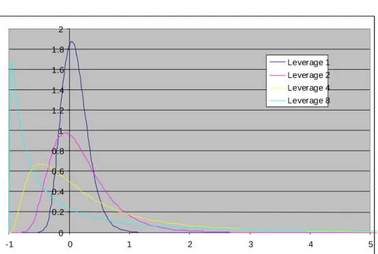
9 is plotted in Figure (1) for different degrees of leverage L.0 0.2 0.4 0.6 0.8 1 1.2 1.4 1.6 1.8 2
-1 0 1 2 3 4 5
Leverage 1 Leverage 2 Leverage 4 Leverage 8
Figure 1: Plot of the profit and loss probability distribution for a leveraged fund for t=1 year, =0.08, =0.2, r=0.02 for leverage factors L=1, L=2, L=4 and L=8. For high degrees of leverage, the probability of making a loss tends to 1 despite the fact that the expected fund value tends to infinity.
It is interesting to note that for L the expected fund value (7) becomes infinite (assuming u>r), whereas the probability of making a loss PL(x=0) 1 according to equation (8).
Hence, highly leveraged funds reveal a profit and loss distribution which is similar to the well-know St. Petersburg paradox, where a very high (infinite) expected profit is combined with a very high probability of making a loss. For that reason, fund managers cannot maximise the expected fund value, but will maximise the expected yearly return of the leveraged fund. The expected growth rate of the fund (6) reads
term Volatility ts financ ing return Leveraged tL
L
r
L
L
F
F
E
t
g
2 cos Re 0)
1
(
2
1
)
1
(
ln
1
10The growth-rate (10) is a quadratic polynomial in the leverage L. As indicated in the introduction, the growth rate of the dynamic leverage strategy is determined by the growth rate of the underlying, the level of refinancing costs and an additional volatility term, which represents a volatility loss if L>1 and a volatility gain for a deleveraged strategy, i.e. 0<L<1.
Equation (10) shows the trade-off the investor faces when choosing his leverage L between pushing the growth rate higher and suffering higher losses due to the increased volatility of the portfolio. Consequently, there is an optimal leverage which maximises the expected growth rate (10):
2
2
1
r
L
opt
11
The sharpe-ratio of the optimally leveraged portfolio reads
2
)
1
(
2
1
optopt
L
r
L
r
g
S
12
Both the outperformance of the leveraged fund over the risk free rate and the volatility of the fund increase linearly in the leverage L and hence would leave the sharpe-ratio unchanged. However, the sharpe-ratio is adversely influenced by the volatility loss in the numerator of the sharpe-ratio (12).
MODEL FOR SHORT LEVERAGE
It is interesting to note that the mathematical description of a leveraged trading strategy (3) can be modified to describe a (leveraged) short fund strategy, which has also become increasingly popular in the ETF market (cf EDHEC 2009). Analogous to long leveraged funds, short funds typically track a (leveraged) short version of a standard equity index.
A short index fund typically borrows and short sells the underlying and invests the fund value plus the proceeds from short selling into the fixed income markets. Analogous to the leveraged fund, the portfolio is rebalanced on a daily basis to ensure a constant leverage with respect to the underlying. Hence, for L < 0 the portfolio strategy reads (cf NYSE Euronext 2008, STOXX 2010):
dF
t
F
tL
(
dt
dW
t)
F
t(
L
1
)
rdt
F
tLbdt
13The trading strategy (13) consists of borrowing L times the underlying asset at a borrowing fee rate b, short selling the L borrowed asset units and investing the proceeds from the short selling plus the fund value into the money market at rate r. The case L= -1 corresponds to a standard short strategy, whereas L< -1 reproduces a leveraged short fund.
The analogous calculations yield the fund value:
L
rt
Lbt
L
L
t
S
S
F
F
L t t 2 00
(
1
)
2
1
)
1
(
exp
14And the expected long term growth rate:
loss V olatility earned I nterest ts Borrowing return LeveragedL
L
r
L
Lb
L
g
2 cos)
1
(
2
1
)
1
(
15Which is maximised by the following optimal leverage factor:
2
2
1
r
b
L
opt
Analogously, the sharpe-ratio for a (leveraged) short strategy reads:
r
b
L
L
r
g
S
opt opt
2)
1
(
2
1
TRANSACTION COSTS
Transactions costs are an important issue when analysing the long term performance of investment products. Generally speaking, standard ETFs tracking a simple equity index typically offer the advantage of very low transaction costs compared to actively managed funds or structured products, in particular ETFs tracking highly liquid blue-chip indices.
The actual impact of transaction costs on the long term performance of tracking funds is transparent in the form of the tracking error that fund companies publish on a regular basis.
As pointed out by Cheng (2009), leveraged and short ETFs can imply significantly higher transaction costs than standard ETFs for an obvious reason: Leveraged and short ETFs typically require a daily re-balancing, thereby creating transaction costs on a daily basis, whereas standard ETFs follow a buy and hold strategy and only have to be re-balanced when the underlying index is rebalanced. The re-balancing frequency of standard indices ranges from monthly to yearly and hence is significantly lower than for leveraged and short indices.
Hence, while neglecting transaction costs for standard ETFs can a feasible simplification, an appropriate model for leveraged and short strategy with daily re-balancing should take re-balancing costs into account. The main problem regarding transaction costs is the fact that they strongly depend on the size of the relevant fund, the way it is managed (i.e. physical replication or swap-based replication) and the type of market access (direct exchange access or access through brokers etc.) and therefore differs significantly across different market participants.
However, to promote a realistic model for transaction costs within the context of leveraged and short funds, one can identify two main drivers for the amount of transaction based losses:
1. The daily turnover Tt in the underlying asset, which is
)
(
t t t t tt
F
L
udt
dW
S
dS
L
F
T
16
2.The costs per transaction volume , which is an institute specific parameter, depending on the size of the fund, the replication strategy and the type of market access.
Hence, the daily transaction costs are the absolute value of the transaction volume (16) times the institute specific transaction cost parameter:
t t t t t
t
F
L
udt
dW
S
dS
L
F
dt
C
17
To estimate the impact of transaction costs on the long term performance of leveraged and short funds, we analyse unit transaction costs ct = Ct / Ft which follow a folded normal distribution and hence the expected value of ct reads:
222
exp
2
2
1
:
L
u
u
u
c
E
c
t18
Hence, to approximate the impact of transactions costs within the framework of leveraged and short indices developed above, one has to include an additional charge cdt into the model. For leveraged indices this is equivalent to increasing the interest rate in the model (3) from r to r+c, for short indices it is equivalent to increasing the cost of borrowing in the model (13) from b to b+c, with c calculated according to equation (18).
It is interesting to note that according to the model (18) unit transaction costs increase in the degree of leverage and the volatility of the underlying index, which is in line with intuition, because higher leverage and higher volatility both increase the average daily turnover.
Numerical examples
As an example we consider the EURO STOXX 50 Total Return Index as an underlying of a leveraged fund strategy with daily re-balancing. To assess the question in how far the optimal leverage depends on the market conditions (i.e. bull market versus bear market), we calculate the performance of a leveraged strategy on the EURO STOXX 50 Index for two time periods – from end of 1991 till end of 2007 (where markets where close to a peak) and from end of 1991 till end of May 2009 (where markets were in a recession). The average index growth rate, interest rate, volatility and the resulting optimal leverage according to formula (11) are summarised in the following table:
Parameter Period 31.12.1991 – 31.12.2007 Period 31.12.1991-30.5.2009
12.39% 8.04%
20.17% 22.25%
r 4.03% 3.95%
Opt. Leverage 2.55 1.33
Table 4: Average growth rate and volatility of the EURO STOXX 50 return index and average interest rate for the indicated time periods and the resulting optimal leverage factor according to (11).
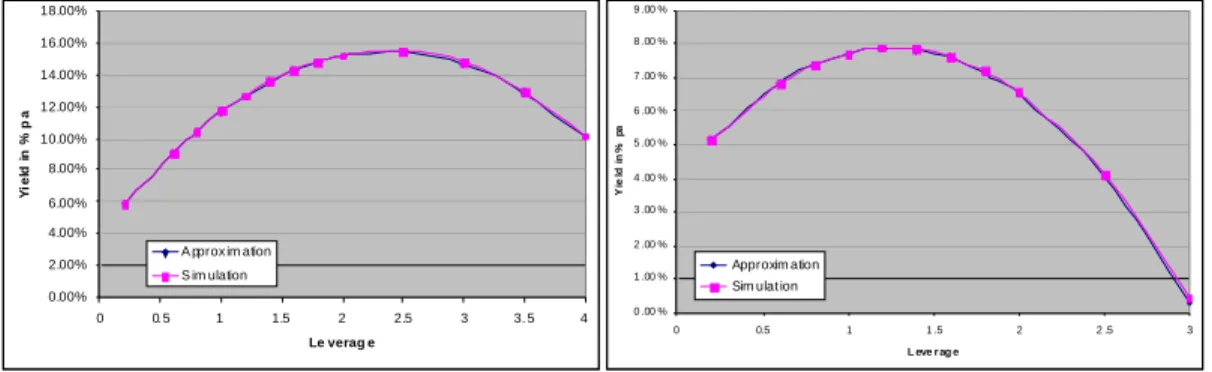
Figure 2 below compares the average yearly performance of the leveraged strategy as a function of the leverage factor calculated by using the approximation formula (6) to the exact simulation of the leveraged strategy for both time periods.
0.00% 2.00% 4.00% 6.00% 8.00% 10.00% 12.00% 14.00% 16.00% 18.00%
0 0. 5 1 1.5 2 2.5 3 3. 5 4
Le verag e
Y
ie
ld
in
%
p
a
A pprox im ation S im ulation
0 .00 % 1 .00 % 2 .00 % 3 .00 % 4 .00 % 5 .00 % 6 .00 % 7 .00 % 8 .00 % 9 .00 %
0 0.5 1 1 .5 2 2 .5 3
L eve r ag e
Y
ie
ld
in
%
p
a
Approxim ation Sim ulat ion
Figure 2: Average yearly performance of a leveraged strategy on the EURO STOXX 50 Return Index as a function of the leverage factor from end of 1991 till end of 2007 (bullish market) on the left and till May 2009 (bear market) on the right, calculated using the approximation (6) versus the exact simulation. In both cases one observes that there is an optimal degree of leverage that optimally exploits the trade-off between higher growth rates and volatility losses.
It is interesting to note from Figure 2 that formula (6) gives a very good approximation of the long term performance of the leveraged strategy. The differences between the approximation and the actual simulation are due to the fact that the derivation of the approximation (6) through Ito’s lemma is based on two simplifying assumptions:
1. Infinitesimal portfolio changes dF in the trading strategy (3), whereas the real world simulation uses a daily re-balancing.
2.The returns of the underlying follow a normal distribution, whereas real world returns are not strictly normal. In particular, real world returns show a heavy tale for negative returns which is amplified by a leveraged trading strategy and hence explains why the fully simulated solution underperforms the approximate solution (6) in Figure 2 – the higher the leverage, the greater the underperformance. Further, the optimal leverage factor strongly depends on the market conditions, i.e. in the bull market of 2007 a fund with a leverage of 2.55 would have performed best over the time period starting end of 1991, whereas only seventeen months later the optimal strategy would have been a leverage of 1.32. This sudden change is explained by formula (6), i.e. the performance of the underlying is geared up by a power of L and hence the downturn due to the market turmoil in 2008 clearly harms a higher leverage more severe than a lower leverage.
To illustrate the advantages of the concept of optimal leverage, we simulate a leveraged fund strategy on the EURO STOXX 50 Return Index according to the strategy (3), where the leverage factor is set to the optimal degree of leverage (11) on a monthly basis. We use implied volatilities as measured by the VSTOXX index (for details see STOXX 2010) as proxy for the volatility , the EONIA rate as refinancing cost r and the annualized life-to-date performance of the underlying index as growth rate . The advantage of using implied lies in their forward-looking character, which means that the strategy will react faster to market turbulences than a strategy using historical volatilities. Transaction costs have been neglected in the following simulations, because they are institute specific as argued in the previous section.
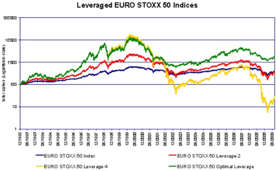
Figure 3 compares the performance of the optimal leverage strategy to the underlying EURO STOXX 50 Return Index and a strategy with a constant leverage factor of two and four. In the numerical simulations a cap of four was applied the optimal leverage factor to limit the risk of investors.
Figure 3: History of the leverage two and leverage four strategy and an optimally leveraged strategy compared to the underlying EURO STOXX 50 Index. In the long run a constant leverage factor does not create any value (leverage two) or even destroys value (leverage 4) due to the volatility related losses, whereas the optimal leverage strategy clearly outperforms the underlying index by using a degree of leverage that is adjusted to the prevailing market environment, in particular to the volatility of the underlying.
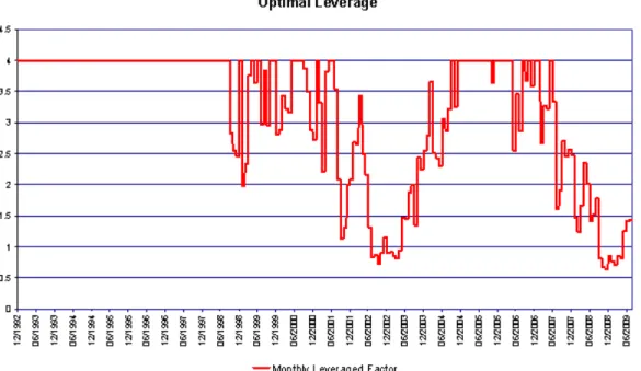
Figure 4 shows the corresponding evolution of the optimal leverage factor.
Figure 4: Optimal leverage factor over time: In bullish markets such as the mid nineties or the rally from 2004 till 2007 the leverage is set to the maximum of four. However, in turbulent markets the optimal leverage factors is clearly lower due to the increased level of volatility. During the market crash of September 2008 the optimal leverage is even below one, i.e. the optimal strategy in that market environment was to de-leverage the fund.
It is interesting to note that the strategy using a constant leverage of two shows approximately the same long-term performance as the underlying index, which means that in the long run the upside potential of higher returns due to leverage are roughly offset by volatility losses. However, the leverage four strategy underperforms the underlying index in the long run, because volatility related losses more than offset the advantage of leveraged returns. This observation reconfirms the results obtained by Cheng (2009), Despande (200) and Lu (2009) for strategies based on a constant leverage factor.
On the other hand, the optimally leveraged strategy outperforms the underlying index in the long run, because it uses a high degree of leverage in bullish markets (i.e. during the mid nineties and during the period from 2003 till 2007), but reduces the leverage significantly in turbulent markets. To conclude, adjusting the leverage factor to market conditions according to the concept of optimal leverage clearly adds value in the long run, in contrast to the strategy of using a constant leverage factor.
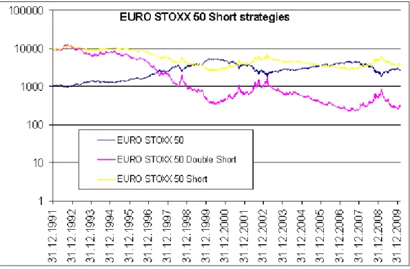
As a final example for analyze the long term performance of a single short strategy and a double short strategy on the EURO STOXX 50 Index in Figure 5. The singe short strategy resembles an inversed version of the underlying index in the short run at each point in time and hence creates value in bear markets. However, in the long run the single short strategy has destroyed value for two reasons: The underlying index
had a positive growth rate over the simulation period and the short strategy suffers from volatility driven losses as explained above. For the double short strategy the volatility driven losses are even higher, explaining the dramatic long run loss of portfolio value over the simulation period. In essence, short ETFs are instruments that are suited as short term trading instruments to profit from bear markets, but are not suited for long term investing.
Figure 5: Simulation of a single short and a double short strategy in comparison to the underlying EURO STOXX 50 Index.
CONCLUSION
The mathematics of dynamic leveraged long or short trading strategies shows a clear trade-off between exploiting the potential of higher returns which grow linearly in the leverage factor and adverse losses due to the volatility of the underlying, which is proportional to the leverage squared. Hence there is an optimal leverage factor which maximises the expected future fund value. Since a leveraged fund strategy gears up the performance of the underlying by a power of the leverage factor, one observes that the optimal leverage strongly depends on the prevailing market conditions, i.e. it is higher in bullish markets and lower in a bearish environment. In particular, the optimal leverage is higher for lower levels of volatility and lower refinancing costs and increases in the expected growth rate of the underlying. It is interesting to note that the simulations we performed indicate that a dynamic leverage strategy pays-off in the long run and throughout the business cycle if the leverage factor is chosen appropriately.
LITERATURE
1. Baxter, M., Rennie, A. (1996) Financial Calculus: An Introduction to Derivative Pricing, Cambridge University Press.
2.Cheng, M., Madhavan, A. (2009) The Dynamics of Leveraged and Inverse-Exchange Traded Funds, Barclays Global Investors.
3.Despande, M., Mallick, D., Bhatia, R. (2009) Understanding Ultrashort ETFs, Barclays Capital Special Report.
4.EDHEC (2009) The EDHEC European ETF Survey 2009.
5.Lu, L, Wang, J., Zhang, G. (2009) Long Term Performance of Leveraged ETFs, Working paper, available at http://ssrn.com/abstract=1344133.
6.NYSE Euronext (2008) Rules for the Leverage indexes. 7. NYSE Euronext (2008) Rules for the Short indexes.
8.STOXX (2019) STOXX Index Guide, ww.stoxx.com/download/indices/rulebooks/djstoxx_indexguide.pdf.
ABOUT THE AUTHOR: Guido Giese
is Director of Research & Development at STOXX Ltd. in Zurich where he is responsible for applied research in the area of asset management and financial products and for the development of new asset
management strategies. Before joining STOXX in 2008, he held managerial positions in various Swiss asset managers and international investment banks in the area of trading and financial products. Guido holds a PhD in applied mathematics from ETH Zurich, an MSc in physics from the University of Heidelberg and an MSc in economics from the University of Hagen.
ABOUT STOXX LIMITED:
STOXX Ltd. is a global index provider, currently calculating a global, comprehensive index family of over 3,700 strictly rules-based and transparent indices. Best known for the leading European equity indices EURO STOXX 50, STOXX Europe 50 and STOXX Europe 600, STOXX Ltd. maintains and calculates the STOXX Global Index family which consists of total market, broad and blue-chip indices for the regions Americas, Europe, Asia, and Pacific, the sub-regions Latin America and BRIC (Brazil, Russia, India and China), as well as global markets.
The STOXX indices are licensed to over 400 companies around the world as underlyings for Exchange Traded Funds (ETFs), Futures & Options, Structured Products and passively-managed investment funds. Three of the top Exchange Traded Funds (ETFs) in Europe and 30 percent of all assets under management are based on STOXX indices. STOXX Ltd. holds Europe's number one and the world's number three position in the derivatives segment.
In addition, STOXX Ltd. is the marketing agent for the indices of Deutsche Boerse AG and SIX Group AG, amongst them the DAX and the SMI indices.