Portfolio Construction Using Stratified Models
Jonathan Tuck
Shane Barratt
Stephen Boyd
January 8, 2021
AbstractIn this paper we develop models of asset return mean and covariance that depend on some observable market conditions, and use these to construct a trading policy that depends on these conditions, and the current portfolio holdings. After discretizing the market conditions, we fit Laplacian regularized stratified models for the return mean and covariance. These models have a different mean and covariance for each market condition, but are regularized so that nearby market conditions have similar models. This technique allows us to fit models for market conditions that have not occured in the training data, by borrowing strength from nearby market conditions for which we do have data. These models are combined with a Markowitz-inspired optimization method to yield a trading policy that is based on market conditions. We illustrate our method on a small universe of 18 ETFs, using four well known and publicly available market variables to construct 10000 market conditions, and show that it performs well out of sample. The method, however, is general, and scales to much larger problems, that presumably would use proprietary data sources and forecasts along with publicly available data.
1
Introduction
Trading policy. We consider the problem of constructing a trading policy that depends on some observable market conditions, as well as the current portfolio holdings. We denote the asset daily returns as yt ∈ Rn, for t = 1, . . . , T. The observable market conditions are
denoted as zt. We assume these are discrete or categorical, so we have zt∈ {1, . . . , K}. We
denote the portfolio asset weights as wt∈Rn, with1Twt= 1, where1 is the vector with all
entries one. The trading policy has the form
T :{1, . . . , K} ×Rn→Rn,
where wt = T(zt, wt−1), i.e., it maps the current market condition and previous portfolio
weights to the current portfolio weights. In this paper we refer toztas the market conditions,
Laplacian regularized stratified model. We model the asset returns, conditioned on market conditions, as Gaussian,
y|z ∼ N(µz,Σz),
with µz ∈ Rn and Σz ∈ Sn++ (the set of symmetric positive definite n×n matrices), z =
1, . . . , K. This is a stratified model, with stratification featurez. We fit this stratifed model,
i.e., determine the meansµ1, . . . , µK and covariances Σ1, . . . ,ΣK, by minimizing the negative
log-likelihood of historical training data, plus a regularization term that encourages nearby market conditions to have similar means and covariances. This technique allows us to fit models for market conditions which have not occured in the training data, by borrowing strength from nearby market conditions for which we do have data. Laplacian regularized stratified models are discussed in, e.g., [DWW14, SS16, TBB21, TB20]. One advantage of Laplacian regularized stratified models is they are interpretable. They are also auditable: we can easily check if the results are reasonable.
This paper. In this paper we present a single example of developing a trading policy as described above. Our example is small, with a universe of 18 ETFs, and we use market conditions that are publicly available and well known. Given the small universe and our use of widely available market conditions, we cannot expect much in terms of performance, but we will see that the trading algorithm performs well out of sample. Our example is meant only as a simple illustration of the ideas; the techniques we decribe can easily scale to a universe of thousands of assets, and use proprietary forecasts in the market conditions.
Outline. We start by reviewing Laplacian regularized models in§2. In§3we describe the data records and dataset we use. In §4 we describe the economic conditions with which we will stratify our return and risk models. In §5 and 6 we describe, fit, and analyze the stratified return and risk models, respectively. In §7 we give the details of how our stratified return and risk models are used to create the trading policyT. We mention a few extensions and variations of the methods described in §8.
1.1
Related work
A number of studies show that the underlying covariances of equities change during different market conditions, such as when the market performs historically well or poorly (a “bull” or “bear” market, respectively), or when there is historically high or low volatility [EHV94,
LS01, AB03, AB04, Bor12]. Modeling the dynamics of underlying statistical properties of assets is an area of ongoing research. Many model these statistical properties as occurring in hard regimes, and utilize methods such as hidden Markov models [RTA98, NML18] or greedy Gaussian segmentation [HNB16] to model the transitions and breakpoints between the regimes. In contrast, this paper assumes a hard regime model of our statistical parameters, but our chief assumption is, informally speaking, that similar regimes have similar statistical parameters.
Asset allocation based on changing market conditions is a sensible method for active portfolio management [AB02,AT11,NHML15,Pet15]. A popular method is to utilize convex optimization control policies to dynamically allocate assets in a portfolio, where the time-varying statistical properties are modeled as a hidden Markov model [NBLM19].
2
Laplacian regularized stratified models
In this section we review Laplacian regularized stratified models, focussing on the specific models we will use; for more detail see [TBB21, TB20]. We are given data records of the form (z, y) ∈ {1, . . . , K} ×Rn, where z is the feature over which we stratify, and y is the outcome. We let θ ∈ Θ denote the parameter values in our model. The stratified model consists of a choice of parameter θz for each value of z. In this paper, we construct two
stratified models. One is for return, where θz ∈Θ =Rn is an estimate or forecast of return,
and the other is for return covariance, where θz ∈ Θ = Sn++ is the inverse covariance or
precision matrix, and Sn++ denotes the set of symmetric positive definite n ×n matrices. (We use the precision matrix since it is the natural parameter in the exponential family representation of a Gaussian, and renders the fitting problems convex.)
To choose the parameters θ1, . . . , θK, we minimize
K
X
k=1
(`k(θk) +r(θk)) +L(θ1, . . . , θK). (1)
Here `k is the loss function, that depends on the training data yi, for zi = k, typically a
negative log-likelihood under our model for the data. The function ris the local regularizer, chosen to improve out of sample performance of the model.
The last term in (1) is the Laplacian regularization, which encourages neighboring values ofz, under some weighted graph, to have similar parameters. It is characterized byW ∈SK, a symmetric weight matrix with zero diagonal entries and nonnegative off-diagonal entries. The Laplacian regularization has the form
L(θ1, . . . , θK) =
1 2
K
X
i,j=1
Wijkθi −θjk2,
where the norm is the Euclidean or `2 norm when θz is a vector, and the Frobenius norm
whenθz is a matrix. We think ofW as defining a weighted graph, with edges associated with
positive entries of W, with edge weight Wij. The larger Wij is, the more encouragement we
give for θi and θj to be close.
When the loss and regularizer are convex, the problem (1) is convex, and so in principle is tractable [BV04]. The distributed method introduced in [TBB21], which exploits the
A Laplacian regularized stratified model typically includes several hyper-parameters, for example that scale the local regularization, or scale some of the entries in W. We adjust these hyper-parameters by choosing some values, fitting the Laplacian regularized stratified model for each choice of the hyper-parameters, and evaluating the true loss function on a (held-out) validation set. (The true loss function is often but not always the same as the loss function used in the fitting objective (1).) We choose hyper-parameters that give the least, or nearly least, true loss on the validation data, biasing our choice toward larger values, i.e., more regularization.
We make a few observations about Laplacian regularized stratified models. First, they are interpretable, and we can check them for reasonableness by examining the valuesθz, and
how they vary with z. At the very least, we can examine the largest and smallest values of each entry (or some function) of θz over z ∈ {1, . . . , K}.
Second, we note that a Laplacian regularized stratified model can be created even when we have no training data for some, or even many, values of z. The parameter values for those values of z are obtained by borrowing strength from their neighbors for which we do have data. In fact, the parameter values for values of z for which we have no data are weighted averages of their neighbors. This implies a number of interesting properties, such as a maximum principle: Any such value lies between the minimum and maximum values of the parameter over those values of z for which we have data.
3
Dataset
Our example considers n = 18 ETFs as the universe of assets,
AGG, DBC, GLD, IBB, ITA, PBJ, TLT, VNQ, VTI, XLB, XLE, XLF, XLI, XLK, XLP, XLU, XLV, XLY.
Each data record has the form (y, z), where y ∈ R18 is the daily return of each asset from market close on the previous day until market close on that day, andz represents the market condition known at the previous day’s market close, described later in §4.
Our dataset spans February 2006 to December 2019, for a total of 3500 data points. We first partition it into two subsets. The first, using data from 2006–2014, is used to fit the return and risk models as well as to choose the hyper-parameters in the return and risk models and the trading policy. The second subset, with data in 2015–2019, is used to test the trading policy. We then randomly partition the first subset into two parts: a training set consisting of 80% of the data records, and a validation set consisting of 20% of the data records. Thus we have three datasets: a training data set with 1780 data points in the date range 2006–2014, a validation set with 446 data points also in the date range 2006–2014, and a test dataset with 1258 data points in the date range 2015–2019. We use 11 years of data to fit our models and choose hyper-parameters, and 5 years of later data to test the trading policy. The return data in the training and validation datasets were winsorized (clipped) at their 1st and 99th percentiles. The return data in the test dataset was not.
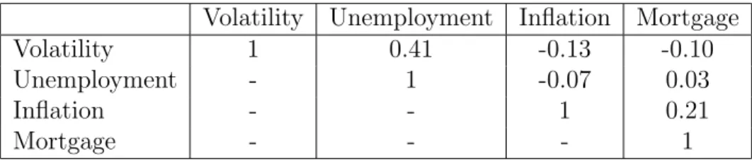
Volatility Unemployment Inflation Mortgage
Volatility 1 0.41 -0.13 -0.10
Unemployment - 1 -0.07 0.03
Inflation - - 1 0.21
Mortgage - - - 1
Table 1: Correlation of the market indicators over the training and validation period, 2006–2014.
4
Stratified market conditions
Each data record also includes the market condition z known on the previous day’s market close. To construct the market conditionz, we start with four (real-valued) market indicators.
Market implied volatility. The volatility of the market is a commonly used economic indicator, with extreme values associated with market turbulence [FSS87, Sch89, AIL99,
CCR20]. Here, volatility is measured by the five-day moving average of the CBOE volatility index (VIX) on the S&P 500 [Exc20].
Unemployment rate. The percentage of adults in the economy who are seeking em-ployment and unemployed is a widely used economic indicator. A high unemem-ployment rate is typically associated with decreased purchasing power and smaller overall economic out-put [Lov76, Cai79, GRV11]. The United States unemployment rate is published by the United States Bureau of Labor Statistics [oLS20b], and updated monthly.
Inflation rate. The inflation rate measures the percentage change of purchasing power in the economy [WS94,BLS96, BLS01, BC03,Hun03,Mah17]. The inflation rate is published by the United States Bureau of Labor Statistics [oLS20a] as the percent change of the consumer price index (CPI), which measures changes in the price level of a representative basket of consumer goods and services, and is updated monthly.
30-year U.S. mortgage rates. This metric is the interest rate charged by a mortgage lender on 30-year mortgages, and the change of this rate is an economic indicator correlated with economic spending [Cav16, SMS17]. The 30-year U.S. mortgage rate are published by the Federal Home Loan Mortgage Corporation, a public government-sponsored enterprise, and is generally updated daily [FRED20].
These four economic indicators are not particularly correlated over the training and validation period, as can be seen in table 1.
2006
2008
2010
2012
2014
2016
2018
2020
Date
1
2
3
4
5
6
7
8
9
10
Decile
vix
unemployment inflation mort30us
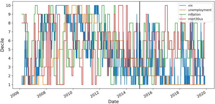
Figure 1: Stratification feature values over time. The vertical line at 2015 separates the training and validation period, 2006–2014 from the test period, 2015-2019.
stratification feature values is thenK = 10×10×10×10 = 10000. We can think of z as a 4-tuple of deciles, in {1, . . . ,10}4, or encoded as a single value z ∈ {1, . . . ,10000}.
The market conditions over the entire dataset are shown in figure 1, with the vertical line at 2015 indicating the boundary between the training and validation period (2006–2014) and the test period (2015–2019). The average value of kzt+1−ztk1 (interpreting them as
in{1, . . . ,10}4) is around 0.62, meaning that on each day, the market conditions change by
around 0.62 deciles.
Data scarcity. The market conditions can take on K = 10000 possible values. In the training/validation datasets, only 346 of 10000 market conditions appear, so there are 9654 market conditions for which there are no data points. The most populated market condition, which corresponds to market conditions (9,4,0,0), contains 62 data points. The average number of data points per market condition in the training/validation data is 0.22.
In the test dataset, only 189 of the economic conditions appear. The average number of data points per market condition in the test dataset it is 0.13. Only nine economic conditions appear in both the training/validation and test datasets. In the test data, there are only 58 days in which the market conditions were observed in the training/validation datasets.
For over 96% of the market conditions, we have no training data. This scarcity of data means that the Laplacian regularization is critical in constructing models of the return and risk that depend on the market conditions.
Regularization graph. Laplacian regularization requires a weighted graph that tells us which market conditions are ‘close’. Our graph is the Cartesian product of four chain graphs, which link each decile of each indicator to its successor (and predecessor). This graph on the 10000 values ofz has 36000 edges. Each edge connects two adjacent deciles of one of our four economic indicators. We assign four different positive weights to the edges, depending on which indicator they link. We denote these as
γvol, γunemp, γinf, γmort. (2)
These are hyper-parameters in our Laplacian regularization. Each of the nonzero entries in the weight matrix W is one of these values. For example, the edge between (3,2,4,6) and (3,2,5,6), which connects two values of z that differ by one decile in Inflation, has weight
γinf.
5
Stratified return model
In this section we describe the stratified return model. The model consists of a mean return vector in µz ∈ R18 for each of K = 10000 different market conditions, for a total of Kn=
180000 parameters.
The loss in (1) is a Huber penalty,
`k(µk) =
X
t:zt=k
1TH(µk−yt),
where H is the Huber penalty (applied entrywise above),
H(z) =
(
z2, |z| ≤M
2M|z| −M2, |z|> M,
where M > 0 is the half-width, which we fix at the reasonable value M = 0.01. (This corresponds to the 69th percentile of absolute return on the training dataset.) We use quadratic or `2 squared local regularization in (1),
r(µk) =γret,lockµkk22,
where the positive regularization weight γret,loc is another hyper-parameter.
The Laplacian regularization contains the four hyper-parameters (2), so overall our strat-ified return model has five hyper-parameters.
5.1
Hyper-parameter search
To choose the hyper-parameters for the stratified return model, we start with a coarse grid search, evaluating all combinations of
γret,loc = 0.001,0.01,0.1,
γvol = 1,10,100,1000,10000,
γunemp = 1,10,100,1000,10000,
γinf = 1,10,100,1000,10000,
γmort = 1,10,100,1000,10000,
a total of 1875 combinations, and selecting the hyper-parameter combination that yielded the largest correlation between the return estimates and the returns over the validation set. (Thus, our true loss is negative correlation of forecast and realized returns.) The hyper-parameters
(γret,loc, γvol, γunemp, γinf, γmort) = (0.01,10,10,1000,1000)
gave the best results over this coarse hyper-parameter grid search.
We then perform a finer hyper-parameter grid search, focusing on hyper-parameters around the best values from the coarse search. We test all combinations of
γret,loc = 0.0075,0.01,0.0125,
γvol = 2,5,10,20,50,
γunemp = 2,5,10,20,50,
γinf = 200,500,1000,2000,5000,
γmort = 200,500,1000,2000,5000,
a total of 1875 combinations. The final hyper-parameter values are
(γret,loc, γvol, γunemp, γinf, γmort) = (0.0075,5,10,1000,1000). (3)
5.2
Final stratifed return model
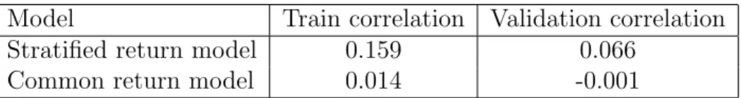
Table 2shows the correlation coefficient of the return estimates to the true returns over the training and validation sets, for the stratified return model and the common return model,
i.e., the empirical mean over the training set. The stratified return model estimates have a larger correlation with the realized returns in both the training set and the validation set. The common return model even has a slightly negative correlation with the true returns on the validation dataset.
Table 3 summarizes some of the statistics of our stratified return model over the 10000 market conditions, along with the common model value. We can see that each forecast varies considerably across the market conditions. Note that the common model values are the averages over the training data; the median, minimum, and maximum are over the 10000 market conditions.
Model Train correlation Validation correlation
Stratified return model 0.159 0.066
Common return model 0.014 -0.001
Table 2: Correlations to the true returns over the training set and the held-out validation set for the return models.
Asset Common Median Min Max
AGG 0.007 0.006 -0.016 0.042
DBC -0.004 0.019 -0.104 0.111
GLD 0.057 0.074 0.015 0.148
IBB 0.077 0.080 -0.039 0.215
ITA 0.048 0.058 -0.110 0.183
PBJ 0.036 0.047 -0.109 0.129
TLT 0.032 0.038 -0.037 0.124
VNQ 0.036 0.038 -0.201 0.162
VTI 0.021 0.046 -0.166 0.150
XLB 0.028 0.061 -0.075 0.206
XLE 0.030 0.074 -0.100 0.228
XLF 0.003 -0.013 -0.246 0.128
XLI 0.027 0.040 -0.123 0.150
XLK 0.033 0.057 -0.131 0.154
XLP 0.037 0.045 -0.060 0.111
XLU 0.015 0.034 -0.096 0.108
XLV 0.045 0.050 -0.061 0.148
XLY 0.043 0.046 -0.140 0.168
Table 3: Return predictions, in percent daily return. The first column gives the common re-turn model; the second, third, and fourth columns give median, minimum, and maximum rere-turn predictions over the 10000 market conditions for the Laplacian regularized stratified model.
6
Stratified risk model
In this section we describe the stratified risk model, i.e., a return covariance that depends on z. For determining the risk model, we can safely ignore the (small) mean return, and assume thatythas zero mean. The model consists of K = 10000 inverse covariance matrices
Σ−k1 = θk ∈ S18++, indexed by the market conditions. Our stratified risk model has Kn(n+
1)/2 = 1710000 parameters.
The loss in (1) is the negative log-likelihood on the training set,
`k(θk) = (nk/2)Tr(SkΣ−k1)−(nk/2) log det(Σ−k1)−(nkn/2) log(2π),
wherenkis the number of data samples withz =k, andSk= n1
k P
t:zt=kyty
T
t is the empirical
covariance matrix of the data y for which z = k. (When nk = 0, we take Sk = 0.) We
found that local regularization did not improve the model performance, so we take local regularization r = 0. All together our stratified risk model has the four Laplacian hyper-parameters (2).
6.1
Hyper-parameter search
We start with a coarse grid search over all 625 combinations of
γvol = 0.1,1,10,100,1000,
γunemp = 0.1,1,10,100,1000,
γinf = 0.1,1,10,100,1000,
γmort = 0.1,1,10,100,1000,
selecting the hyper-parameter combination with the smallest negative log-likelihood (our true loss) on the validation set. The hyper-parameters
(γvol, γunemp, γinf, γmort) = (1,1,100,100)
gave the best results.
We then perform a fine search, focusing on hyper-parameter value near the best values from the coarse search. We evaluate all 625 combinations of
γvol = 0.2,0.5,1,2,5,
γunemp = 0.2,0.5,1,2,5,
γinf = 20,50,100,200,500,
γmort = 20,50,100,200,500.
For the stratified risk model, the final hyper-parameter values chosen are (γvol, γunemp, γinf, γmort) = (1,0.2,100,50).
These hyper-parameter values are quite different from the last four chosen for the stratified return model, given in (3), even when scaled.
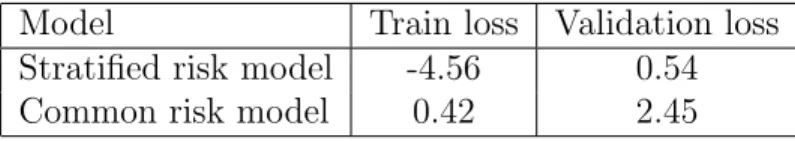
Model Train loss Validation loss
Stratified risk model -4.56 0.54
Common risk model 0.42 2.45
Table 4: Average negative log-likelihood over the training and validation sets for the stratified and common risk models.
6.2
Final stratified risk model
Table 4 shows the average negative log likelihood over the training and held-out validation sets, for both the stratified risk model and the common risk model, i.e., the empirical covariance. We can see that the stratified risk model has substantially better true loss on the training and validation sets.
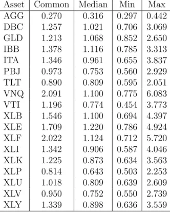
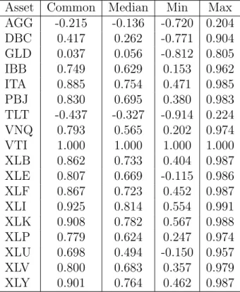
Table 5summarizes some of the statistics of our stratified return model asset volatilities,
i.e., ((Σz)ii)1/2, expressed as daily percentages, over the 10000 market conditions, along with
the common model asset volatilities. We can see that the predictions vary considerably across the market conditions, with a few varying by a factor almost up to ten. Table 6
summarizes the same statistics for the correlation of each asset with VTI, a broad market ETF. Here we see dramatic variation, for example, the correlation between GLD and VTI varies from -81% to +81% over the market conditions.
Asset Common Median Min Max
AGG 0.270 0.316 0.297 0.442
DBC 1.257 1.021 0.706 3.069
GLD 1.213 1.068 0.852 2.650
IBB 1.378 1.116 0.785 3.313
ITA 1.346 0.961 0.655 3.837
PBJ 0.973 0.753 0.560 2.929
TLT 0.890 0.809 0.595 2.051
VNQ 2.091 1.100 0.775 6.083
VTI 1.196 0.774 0.454 3.773
XLB 1.546 1.100 0.694 4.397
XLE 1.709 1.220 0.786 4.924
XLF 2.022 1.124 0.712 5.720
XLI 1.342 0.906 0.587 4.046
XLK 1.225 0.873 0.634 3.563
XLP 0.814 0.643 0.503 2.253
XLU 1.018 0.809 0.639 2.609
XLV 0.950 0.752 0.550 2.739
XLY 1.339 0.898 0.636 3.559
Table 5: Forecasts of volatility, expressed in percent daily return. The first column gives the com-mon model; the second, third, and fourth columns give median, minimum, and maximum volatility predictions over the 10000 market conditions for the Laplacian regularized stratified model.
Asset Common Median Min Max
AGG -0.215 -0.136 -0.720 0.204
DBC 0.417 0.262 -0.771 0.904
GLD 0.037 0.056 -0.812 0.805
IBB 0.749 0.629 0.153 0.962
ITA 0.885 0.754 0.471 0.985
PBJ 0.830 0.695 0.380 0.983
TLT -0.437 -0.327 -0.914 0.224
VNQ 0.793 0.565 0.202 0.974
VTI 1.000 1.000 1.000 1.000
XLB 0.862 0.733 0.404 0.987
XLE 0.807 0.669 -0.115 0.986
XLF 0.867 0.723 0.452 0.987
XLI 0.925 0.814 0.554 0.991
XLK 0.908 0.782 0.567 0.988
XLP 0.779 0.624 0.247 0.974
XLU 0.698 0.494 -0.150 0.957
XLV 0.800 0.683 0.357 0.979
XLY 0.901 0.764 0.462 0.987
Table 6: Forecasts of correlations with the broad market index VTI. The first column gives the common model; the second, third, and fourth columns give median, minimum, and maximum correlation predictions over the 10000 market conditions for the Laplacian regularized stratified model.
7
Trading policy and backtest
7.1
Trading policy
In this section we give the details of how we use our stratified return and risk models to construct the trading policy T. We incorporate cash into our portfolio, so here we consider
n+ 1 = 19 assets. The cash asset has zero return and risk, i.e., (µz)19= 0, and Σz includes
a zero last row and column.
At the beginning of each dayt, we use the previous day’s market conditionsztto allocate
our current portfolio according to the weightswt, computed as the solution of the
Markowitz-inspired problem [BBD+17]
maximize µT
ztw−γscκ
T(w)
−−γtcτT|w−wt−1|
subject to wTΣ
ztw≤σ
2, 1Tw= 1,
kwk1 ≤Lmax, wmin ≤w≤wmax,
(4)
with optimization variable w∈R19, wherew− = max{0,−w} (elementwise), and the abso-lute value is elementwise. We describe each term and constraint below.
• Return forecast. The first term in the objective,µT
ztw, is the expected return under our
forecast mean, which depends on the current market conditions.
• Shorting cost. The second term γscκT(w)− is a shorting cost, with κ∈R19+ the vector
of shorting cost rates. The positive hyper-parameter γsc scales the shorting cost term,
and is used to control our shorting aversion.
• Transaction cost. The third termγtcτT|w−wt−1|is a transaction cost, withτ ∈R19+ the
vector of transaction cost rates. The positive hyper-parameterγtcscales the transaction
cost term, and is used to control the turnover.
• Risk limit. The constraint wTΣ
zw ≤σ2 limits the (daily) risk (under our risk model,
which depends on market conditions) to σ, which corresponds to an annualized risk of
√
250σ.
• Leverage limit. The constraint kwk1 ≤ Lmax limits the portfolio leverage, or
equiva-lently, it limits the total short position 1T(w)− to no more than (L−1)/2.
• Position limits. The constraint wmin ≤ w ≤ wmax (interpeted elementwise) limits the
individual weights.
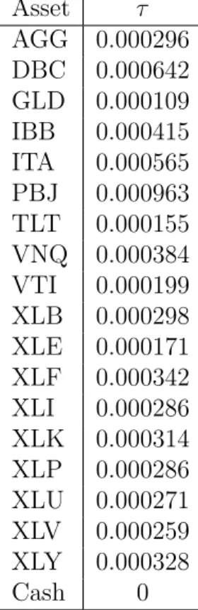
Parameters. Some of the constants in the trading policy (4) we simply fix to reasonable values. We fix the shorting cost rate vector to (0.0005)1, i.e., 5 basis points for each asset. The transaction cost rate vectorτ, shown summarized in table7, is taken to be one-half the average bid-ask spread of each asset over the training period, with non-cash entries ranging from around 0.00011 to 0.00096 (1.1 to 9.6 basis points), with a mean of 0.00035 (3.5 basis
Asset τ
AGG 0.000296
DBC 0.000642
GLD 0.000109
IBB 0.000415
ITA 0.000565
PBJ 0.000963
TLT 0.000155
VNQ 0.000384
VTI 0.000199
XLB 0.000298
XLE 0.000171
XLF 0.000342
XLI 0.000286
XLK 0.000314
XLP 0.000286
XLU 0.000271
XLV 0.000259
XLY 0.000328
Cash 0
Table 7: The transaction cost rate vector τ, which is taken to be one-half the average bid-ask spread of each asset over the training period. We assume that there is no cost to trade cash.
points). We takeσ = 0.005, which corresponds to an annualized volatility of√250σ, around 7.9%. We take Lmax= 2, which means the total short position cannot exceed one half of the
portfolio value. (A portfolio with a leverage of 2 satisfying 1Tw = 1 is commonly referred
to as a 150/50 portfolio.) We fix the position limits as wmin = −0.251 and wmax = 0.31,
meaning we cannot short any asset by more than 0.25 times the portfolio value, and we cannot hold more than 0.3 times the portfolio value of any asset.
Hyper-parameters. Our trading policy has two hyper-parameters, γsc and γtc, which
control our aversion to shorting and trading, respectively.
7.2
Backtests
Backtests are carried out starting from a portfolio of all cash, w = e19, and a starting
portfolio value of v = 1. On day t, after computing wt as the solution to (4), we compute
the value of our portfolio vt by
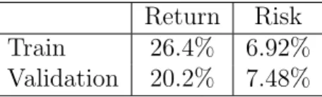
Return Risk
Train 26.4% 6.92%
Validation 20.2% 7.48%
Table 8: Annualized return and risk for the stratified model policy over the train and validation periods.
and transaction costs. In particular, our backtests take shorting and transaction costs into account. (In fact, the actual bid-ask spreads over the test period were smaller than the ones we use in our backtest, which were the average bid-ask spreads over the training period, so our backtests are conservative, i.e., take into account more transaction cost than would actually have been realized.)
Our backtest is a bit simplified. Our simulation assumes dividend reinvestment. We account for the shorting and transaction costs by adjusting the portfolio return, which is equivalent to splitting these costs across the whole portfolio. A slightly more accurate backtest would be obtained using the realized average bid-ask spread on each trading day, and more carefully accounting for the costs using the cash asset. For portfolios of very high value, we would add an additional nonlinear transaction cost term, for example proportional to the 3/2-power of |wt−wt−1| [BBD+17].
7.3
Hyper-parameter selection
To choose values of the two hyper-parameters in the trading policy, we carry out multiple backtest simulations over the training set. We evaluate these backtest simulations by their realized return (net, including costs) over the validation set.
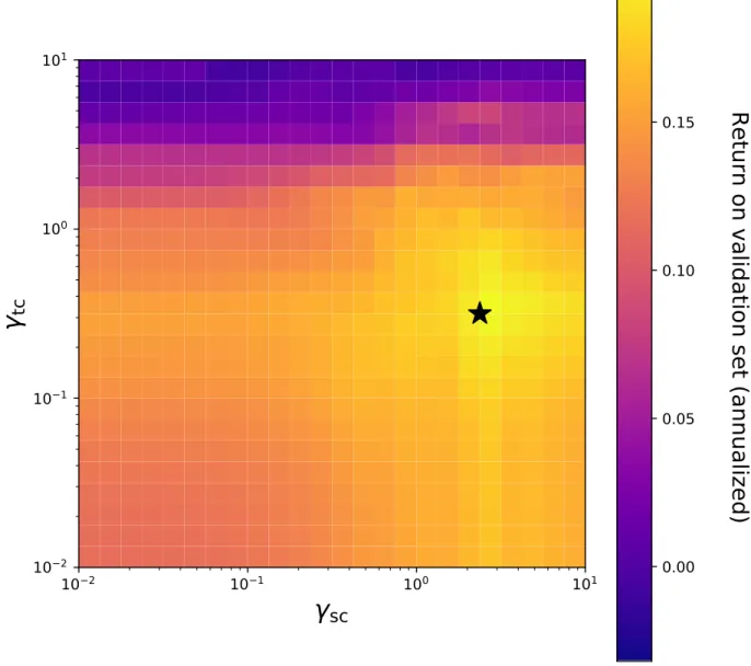
We perform a grid search, testing all 625 pairs of 25 values of each hyper-parameter logarithmically spaced from 0.1 to 10. The annualized return on the validation set, as a function of the hyper-parameters, are shown in figure 2. We choose the final values
γsc= 2.37, γtc = 0.32,
shown on figure2 as a star.
These values are themselves interesting. Roughly speaking, we should plan our trades as if the shorting cost were more twice the actual cost, and the transaction cost is only a third of the true transaction cost. The latter suggests that the trading policy wants to trademore. Indeed the blue and purple band at the top of the heat map, which indicates poor validation performance when the transaction cost parameter is too high, i.e., the policy does not trade enough, confirms that the performance depends on trading enough.
Table 8gives the annualized return and risk for the policies over the train and validation periods. Not surpisingly we see slightly worse performance in the validation period, with a bit more risk and a bit less return.
Common model trading policy. We will compare our stratified model trading policy to a common model trading policy, which uses the constant return and risk models, along
10
210
110
010
1sc
10
210
110
010
1tc
0.00
0.05
0.10
0.15
0.20
Return on validation set (annualized)
Figure 2: Heatmap of the annualized return on the validation set as a function of the two hyper-parameters γsc and γtc. The star shows the hyper-parameter combination used in our trading policy.
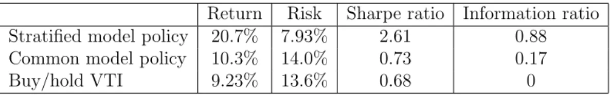
Return Risk Sharpe ratio Information ratio
Stratified model policy 20.7% 7.93% 2.61 0.88
Common model policy 10.3% 14.0% 0.73 0.17
Buy/hold VTI 9.23% 13.6% 0.68 0
Table 9: Annualized return, risk, Sharpe ratios, and information ratios for the three policies for the test period (2015–2019).
with the same Markowitz policy (4). In this case, none of the parameters in the optimization problem change with market conditions, and the only parameter that changes in different days is wt−1, the previous day’s asset weights, which enters into the transaction cost.
We also perform a grid search for this trading policy, over the same 625 pairs of the hyper-parameters. For the common model trading policy, we choose the final values
γsc = 3.16, γtc= 0.074.
7.4
Final trading policy results
We re-fit our stratified risk and return models, utilizing all of the data in the training and validation sets, using the hyper-parameters selected in§5.1and§6.1. We backtest our trading policy on the test dataset, which includes data from 2015–2019. We remind the reader that no data from this date range was used to create, tune, or validate any of the models, or to choose any hyper-parameters. For comparison, we also give results of a backtest using the constant return and risk models, as well as just holding VTI, a total stock market fund.
Figure3 plots the economic conditions over the test period (top) as well as the portfolio value for our stratified model, common model, and VTI (bottom). The superior performance of the stratified model policy, e.g., higher return and lower volatility, is visually evident in this plot. We see that the stratified model policy sails through several market downturns relatively unscathed, with substantially smaller drawdowns in value, measured both in depth and time. It is impressive that the policy avoids the downturn in the end of 2019, since the policy is based on data that is more than 4 years old, i.e., prior to 2015.
Table 9 shows the annualized return, annualized risk, annualized Sharpe ratio (return divided by risk), and information ratio with respect to VTI (return of the policy minus VTI, divided by risk) for the three policies over the test period. The return and risk values are quite consistent with those from the validation period. We remind the reader that we are fully accounting for the shorting and transaction cost, so the turnover of the policy is accounted for in these backtest metrics.
The results are impressive for several reasons. First, we are using a very small universe of only 18 ETFs. Second, our trading policy uses only four widely available market conditions, and indeed, only their deciles. Third, the policy was entirely developed using data prior to 2015, with no adjustments made for the next five years. (In actual use, one would likely re-train the model periodically, perhaps every quarter or year.)
1
2
3
4
5
6
7
8
9
10
Economic conditions decile
Volatility Unemployment Inflation Mortgage
2015
2016
2017
2018
2019
2020
Date
1.00
1.25
1.50
1.75
2.00
2.25
2.50
2.75
Portfolio value
Stratified model policy VTI
Common model policy
Figure 3: Plot of economic conditions (top) and results of the backtest for the stratified model, the common model, and buying/holding VTI (bottom), over the test period.
0.2
0.1
0.0
0.1
0.2
0.3
Stratified model
holdings
2015
2016
2017
2018
2019
2020
Date
0.00
0.05
0.10
0.15
0.20
0.25
0.30
Common model
holdings
Figure 4: Asset weights of the stratified model policy (top) and of the common model policy (bottom), over the test period. The first time period asset weights, which are all cash, are not shown.
Comparison of stratified and constant policies. In figure4, we plot the asset weights of the stratified model policy (top) and of the common model policy (bottom), over the test period. The top plot shows that the weights in the stratified policy change considerably with market conditions. The only asset that is shorted to a significant degree is XLF (financials, shown in orange), and only in periods of market turbulence. The common model policy is concentrated in just four assets, GLD (gold), IBB (biotech), ITA (aerospace/defense), and XLY (consumer discretionary), and never shorts any assets, i.e., is long only.
Factor analysis. We fit a linear regression model of the returns of the three policies over the test set to four of the Fama-French factors [FF92, FF93, Fre21]:
Factor Stratified model policy Common model policy VTI
MKTRF 0.19727 0.88586 0.98122
SMB 0.05369 0.21655 -0.02124
HML -0.03469 -0.31778 -0.00454
UMD -0.00983 -0.06391 0.00022
Alpha 0.000741 0.000008 -0.000042
Table 10: The top four rows give the regression model coefficients of the portfolio returns on the Fama-French factors; the fifth row gives the intercept or alpha value.
• SMB, the return on a portfolio of small size stocks minus a portfolio of big size stocks,
• HML, the return on a portfolio of value stocks minus a portfolio of growth stocks, and
• UMD, the return on a portfolio of high momentum stocks minus a portfolio of low or negative momentum stocks.
We also include an intercept term, commonly referred to as alpha. Table10gives the results of these fits. While the MKTRF coeficients for the common model policy and buying and holding VTI are relatively close to 1, the MKTRF coefficient for the stratified model policy is approximately 0.2,i.e., the returns of the stratified model policy are relatively uncorrelated with the market. The stratified model policy returns are also relatively uncorrelated with the factors SMB, HML, and UMD. Its alpha is around 18.5% annualized.
8
Extensions and variations
We describe some extensions and variations on our method below.
Multi-period optimization. For simplicity we use a policy that is based on solving a single-period Markowitz problem. The entire method immediately extends to policies based on multi-period optimization. For example, we would fit separate stratified models of return and risk for the next 1 day, 5 day, 20 day, and 60 day periods (roughly daily, weekly, monthly, quarterly), all based on the same current market conditions. These data are fed into a multi-period optimizer as described in [BBD+17].
Joint modeling of return and risk. In this paper we created separate Laplacian regu-larized stratified models for return and risk. The advantage of this approach is that we can judge each model separately (and with different true objectives), and use different hyper-parameter values. It is also possible to fit the return mean and covariance jointly, in one stratified model, using the natural parameters in the exponential family for a Gaussian, Σ−1
Low-dimensional economic factors. When just a handful (such as in our example, four) base quantities are used to construct the stratified market conditions, we can bin and grid the values as we do in this paper. This simple stratification of market conditions preserves interpretability. If we wish to include more raw data in our stratification of market conditions, simple binning and enumeration is not practical. Instead we can use several techniques to handle such situations. The simplest is to perform dimensionality-reduction on the (higher-dimensional) economic conditions, such as principal component analysis [Pea01] or low-rank forecasting [BDB20], and appropriately bin these low-dimensional economic conditions. These economic conditions may then be related on a graph with edge weights decided by an appropriate method, such as nearest neighbor weights.
Structured covariance estimation. It is quite common to model the covariance matrix of returns as having structure, e.g., as the sum of a diagonal matrix plus a low rank ma-trix [RSV12, FLL16]. This structure can be added by a combination of introducing new variables to the model and encoding constraints in the local regularization. In many cases, this structure constraint turns the stratified risk model fitting problem into a non-convex problem, which may be solved approximately.
Multi-linear interpolation. In the approach presented above, the economic conditions are categorical, i.e., take on one of K = 10000 possible values at each time t, based on the deciles of four quantities. A simple extension is to use multi-linear interpolation [WZ88,
Dav97] to determine the return and risk to use in the Markowitz optimizer. Thus we would use the actual quantile of the four market quantiities, and not just their deciles. In the case of risk, we would apply the interpolation to the precision matrix Σ−t1, the natural parameter in the exponential family description of a Gaussian.
End-to-end hyper-parameter optimization. In the example presented in this paper there are a total of 11 hyper-parameters to select. We keep things simple by separately optimizing the hyper-parameters for the stratified return model, the stratified risk model, and the trading policy. This approach allows each step to be checked independently. It is also possible to simultaneously optimize all of the hyper-parameters with respect to a single backtest, using, for example, CVXPYlayers [AAB+19,ABBS20] to differentiate through the
trading policy.
Stratified ensembling. The methods described in this paper can be used to combine or emsemble a collection of different return forecasts or signals, whone performance varies with market (or other) conditions. We start with a collection of return predictions, and combine these (ensemble them) using weights that are a function of the market conditions. We develop a stratified selection of the combining weights.
9
Conclusions
We argue that stratified models are interesting and useful in portfolio construction and finance. They can contain a large number of parameters, but unlike, say, neural networks, they are fully interpretable and auditable. They allow arbitrary variation across market conditions, with Laplacian regularization there to help us come up with reasonable models even for market conditions for which we have no training data. The maximum principle mentioned on page 4 tells us that a Laplacian regularized stratified model will never do anything crazy when it encounters values of z that never appeared in the training data. Instead it will use a weighted sum of other values for which we do have training data. These weights are not just any weights, but ones carefully chosen by validation.
The small but realistic example we have presented is only meant to illustrate the ideas. The very same ideas and method can be applied in far more complex and sophisticated settings, with a larger universe of assets, a more complex trading policy, and incorporating proprietary data and forecasts.
Acknowledgements
The authors gratefully acknowledge discussions with and suggestions from Ronald Kahn, Raffaele Savi, and Andrew Ang. Jonathan Tuck is supported by the Stanford Graduate Fellowship in Science and Engineering.
References
[AAB+19] A. Agrawal, B. Amos, S. Barratt, S. Boyd, S. Diamond, and Z. Kolter.
Differen-tiable convex optimization layers. InAdvances in Neural Information Processing Systems, 2019.
[AB02] A. Ang and G. Bekaert. International asset allocation with regime shifts. The Review of Financial Studies, 15(4):1137–1187, July 2002.
[AB03] A. Ang and G. Bekaert. How do regimes affect asset allocation? Technical Report 10080, National Bureau of Economic Research, November 2003.
[AB04] A. Ang and G. Bekaert. How regimes affect asset allocation. Financial Analysts Journal, 60(2):86–99, 2004.
[ABBS20] A. Agrawal, S. Barratt, S. Boyd, and B. Stellato. Learning convex optimization control policies. In Proceedings of the 2nd Conference on Learning for Dynamics and Control, volume 120 of Proceedings of Machine Learning Research, pages 361–373, 10–11 Jun 2020.
[AIL99] R. Aggarwal, C. Inclan, and R. Leal. Volatility in emerging stock markets. The Journal of Financial and Quantitative Analysis, 34(1):33–55, 1999.
[AT11] A. Ang and A. Timmermann. Regime changes and financial markets. Technical Report 17182, National Bureau of Economic Research, June 2011.
[BBD+17] S. Boyd, E. Busseti, S. Diamond, R. Kahn, K. Koh, P. Nystrup, and J. Speth.
Multi-period trading via convex optimization. Foundations and Trends in Opti-mization, 3(1):1–76, 2017.
[BC03] J. Boyd and B. Champ. Inflation and financial market performance: what have we learned in the last ten years? Technical Report 0317, Federal Reserve Bank of Cleveland, 2003.
[BDB20] S. Barratt, Y. Dong, and S. Boyd. Low rank forecasting. Manuscript, 2020. [BLS96] J. Boyd, R. Levine, and B. Smith. Inflation and financial market performance.
Technical report, Federal Reserve Bank of Minneapolis, October 1996.
[BLS01] J. Boyd, R. Levine, and B. Smith. The impact of inflation on financial sector performance. Journal of Monetary Economics, 47(2):221 – 248, 2001.
[Bor12] L. Borland. Statistical signatures in times of panic: markets as a self-organizing system. Quantitative Finance, 12(9):1367–1379, October 2012.
[BV04] S. Boyd and L. Vandenberghe. Convex Optimization. Cambridge University Press, 2004.
[Cai79] G. Cain. The unemployment rate as an economic indicator. Monthly Labor Review, 102(3):24–35, 1979.
[Cav16] G. La Cava. Housing prices, mortgage interest rates and the rising share of capital income in the United States. BIS Working Papers 572, Bank for International Settlements, July 2016.
[CCR20] D. Chun, H. Cho, and D. Ryu. Economic indicators and stock market volatility in an emerging economy. Economic Systems, 44(2):100788, 2020.
[Dav97] S. Davies. Multidimensional triangulation and interpolation for reinforcement learning. In M. C. Mozer, M. I. Jordan, and T. Petsche, editors, Advances in Neural Information Processing Systems 9, pages 1005–1011. MIT Press, 1997. [DWW14] P. Danaher, P. Wang, and D. Witten. The joint graphical lasso for inverse
covariance estimation across multiple classes. Journal of the Royal Statistical Society, 76(2):373–397, 2014.
[EHV94] C. Erb, C. Harvey, and T. Viskanta. Forecasting international equity correlations.
Financial Analysts Journal, 50(6):32–45, 1994.
[Exc20] Chicago Board Options Exchange. CBOE volatility index. http://www.cboe. com/vix, 2020.
[FF92] E. Fama and K. French. The cross-section of expected stock returns. the Journal of Finance, 47(2):427–465, 1992.
[FF93] E. Fama and K. French. Common risk factors in the returns on stocks and bonds.
Journal of Financial Economics, 33(1):3–56, 1993.
[FLL16] J. Fan, Y. Liao, and H. Liu. An overview of the estimation of large covariance and precision matrices. The Econometrics Journal, 19(1):C1–C32, 2016.
[Fre21] K. French. Description of Fama/French factors.https://mba.tuck.dartmouth. edu/pages/faculty/ken.french/data_library.html#Research, 2021.
[FRED20] Federal Reserve Bank of St. Louis Federal Reserve Economic Data. 30-year fixed rate mortgage average in the United States (MORTGAGE30US). https: //fred.stlouisfed.org/series/MORTGAGE30US, 2020.
[FSS87] K. French, W. Schwert, and R. Stambaugh. Expected stock returns and volatility.
Journal of Financial Economics, 19(1):3, 1987.
[GRV11] D. Gatti, C. Rault, and A.-G. Vaubourg. Unemployment and finance: how do fi-nancial and labour market factors interact? Oxford Economic Papers, 64(3):464– 489, 09 2011.
[HNB16] D. Hallac, P. Nystrup, and S. Boyd. Greedy gaussian segmentation of multivari-ate time series. Advances in Data Analysis and Classification, 13, 10 2016. [Hun03] F.-S. Hung. Inflation, financial development, and economic growth. International
Review of Economics & Finance, 12(1):45 – 67, 2003.
[Lov76] J. Lovati. The unemployment rate as an economic indicator. Federal Reserve Bank of St. Louis, 58(Sep):2–9, 1976.
[LS01] F. Longin and B. Solnik. Correlation structure of international equity markets during extremely volatile periods. Journal of Finance, 56(2):649–676, April 2001. [Mah17] H. Mahyar. The Effect Of Inflation On Financial Development Indicators In Iran
(2000-2015). Studies in Business and Economics, 12(2):53–62, August 2017. [Mar52] H. Markowitz. Portfolio selection. The Journal of Finance, 7(1):77–91, 1952. [NBLM19] P. Nystrup, S. Boyd, E. Lindstr¨om, and H. Madsen. Multi-period portfolio
selection with drawdown control. Annals of Operations Research, 282(1):245– 271, November 2019.
[NHML15] P. Nystrup, B. Hansen, H. Madsen, and E. Lindstr¨om. Regime-based versus static asset allocation: Letting the data speak. The Journal of Portfolio Management, 42(1):103–109, 2015.
[NML18] P. Nystrup, H. Madsen, and E. Lindstr¨om. Dynamic portfolio optimization across hidden market regimes. Quantitative Finance, 18(1):83–95, 2018.
[oLS20a] United States Bureau of Labor Statistics. Consumer price index. https://www. bls.gov/cpi/, 2020.
[oLS20b] United States Bureau of Labor Statistics. Employment situation summary.
https://www.bls.gov/news.release/empsit.nr0.htm, 2020.
[Pea01] K. Pearson. On lines and planes of closest fit to systems of points in space. The London, Edinburgh, and Dublin Philosophical Magazine and Journal of Science, 2(11):559–572, 1901.
[Pet15] G. Petre. A case for dynamic asset allocation for long term investors. Procedia Economics and Finance, 29:41 – 55, 2015.
[RSV12] E. Richard, P.-A. Savalle, and N. Vayatis. Estimation of simultaneously sparse and low rank matrices. In Proceedings of the 29th International Conference on Machine Learning, ICML’12, page 51–58, Madison, WI, USA, 2012. Omnipress.
[RTA98] T. Ryden, T. Terasvirta, and S. Asbrink. Stylized facts of daily return series and the hidden markov model. Journal of Applied Econometrics, 13(3):217–244, 1998.
[Sch89] W. Schwert. Why does stock market volatility change over time? The Journal of Finance, 44(5):1115–1153, 1989.
[SMS17] G. Sutton, D. Mihaljek, and A. Subelyt˙e. Interest rates and house prices in the United States and around the world. BIS Working Papers 665, Bank for International Settlements, October 2017.
[SS16] T. Saegusa and A. Shojaie. Joint estimation of precision matrices in heteroge-neous populations. Electronic Journal of Statistics, 10(1):1341–1392, 2016. [TB20] J. Tuck and S. Boyd. Fitting Laplacian regularized stratified Gaussian models.
arXiv, 2020. Manuscript.
[TBB21] J. Tuck, S. Barratt, and S. Boyd. A distributed method for fitting Laplacian regularized stratified models. Journal of Machine Learning Research, 2021. To appear.
[WS94] M. Wynne and F. Sigalla. The consumer price index. Economic and Financial Policy Review, 2:1–22, Feb 1994.
[WZ88] A. Weiser and S. Zarantonello. A note on piecewise linear and multilinear table interpolation in many dimensions. Mathematics of Computation, 50(181):189– 196, 1988.