arXiv:0905.2430v1 [math-ph] 14 May 2009
Using the Schramm-Loewner evolution to explain
certain non-local observables in the 2d critical Ising
model
Michael J. Kozdron
∗Department of Mathematics & Statistics, College West 307.14 University of Regina, Regina, SK S4S 0A2 Canada
Abstract
We present a mathematical proof of theoretical predictions made by Arguin and Saint-Aubin, as well as by Bauer, Bernard, and Kyt¨ol¨a, about certain non-local observ-ables for the two-dimensional Ising model at criticality by combining Smirnov’s recent proof of the fact that the scaling limit of critical Ising interfaces can be described by chordal SLE3 with Kozdron and Lawler’s configurational measure on mutually avoid-ing chordal SLE paths. As an extension of this result, we also compute the probability that an SLEκ path (with 0< κ≤4) and a Brownian motion excursion do not intersect.
1
Introduction
“Though one can argue whether the scaling limits of interfaces in the Ising model are of physical relevance, their identification opens possibility for computation of correlation functions and other objects of interest in physics.”
S. Smirnov (2007)
The Schramm-Loewner evolution (SLE) is a one-parameter family of random growth pro-cesses in two dimensions introduced by O. Schramm [21] while considering possible scaling limits of loop-erased random walk. In the past several years, SLE techniques have been successfully applied to analyze a variety of two-dimensional statistical mechanics models including percolation, the Ising model, the Q-state Potts model, uniform spanning trees, loop-erased random walk, and self-avoiding walk. Furthermore, SLE has provided a mathe-matically rigorous framework for establishing various predictions made by two-dimensional conformal field theory (CFT), and much current research is being done to further strengthen and explain the links between SLE and CFT; see, for example, [9, 10, 11, 17].
In 2002, L.-P. Arguin and Y. Saint-Aubin [3] examined non-local observables in the 2d critical Ising model and using only techniques from conformal filed theory, they derived ex-pressions for such things as the crossing probability of Ising clusters and contours intersecting the boundary of a cylinder. In particular, no mention of SLE was made in that work. In 2005, also using techniques exclusive to conformal field theory, D. Bauer, D. Bernard, and K. Kyt¨ol¨a [4] studied multiple Schramm-Loewner evolutions and statistical mechanics mar-tingales. One consequence of their investigation was the computation of arch probabilities
(using their language) for the critical Ising model.
The primary purpose of the present work is to explain how the results of Arguin and Saint-Aubin [3] as well as Bauer, Bernard, and Kyt¨ol¨a [4] for the Ising model can be derived in a mathematically rigorous manner by combining a recent result of S. Smirnov [22] with the configurational measure on multiple SLE paths introduced by M. Kozdron and G. Lawler [16]. As an extension of this result, we also calculate the probability that an SLEκ path (with
0< κ≤4) and a Brownian excursion do not intersect.
1.1
Towards a possible definition of a partition function for SLE
In the case of a statistical mechanics lattice model, there are only a finite number of possible configurations. (Although this number is enormous, it is still finite.) Therefore, if a particular configuration ω′
is given weight exp{−H(ω′
)/T} where T is the temperature and H is the Hamiltonian, the probability of observing ω′
is
P{ω′
}= exp{−H(ω ′
)/T} P
ωexp{−H(ω)/T}
= exp{−H(ω ′
)/T}
Z(T) . (1) The normalizing factor Z(T) is called the partition function and it is well-known that this quantity encodes the statistical properties of a system in thermodynamic equilibrium.
However, in the scaling limit as the lattice spacing shrinks to 0, the “number” of config-urations becomes infinite. From a physical point-of-view, when working with an “infinite” system one needs an “infinite” term to be factored out so that the result is finite. The infinite factor, however, needs to be independent from the temperature, the shape of the domain, and other physically relevant quantities. Unfortunately, there is no consistent definition of partition function in physics and so the term is often used rather loosely, especially in the context of infinite systems.
As such, it is a challenge to mathematicians to make precise sense of what might be rea-sonably called apartition function for SLE. One way is to construct an object that possesses some of the characteristics of a partition function (in the physical sense). For instance, it might be chosen to satisfy a certain (physically relevant) differential equation. In the present manuscript we introduce an object that can, in this sense, be called apartition function for multiple SLE. Mathematically, it is a normalizing factor that arises in the construction of a finite measure on multiple SLE paths, and satisfies the same differential equation as in Ar-guin and Saint-Aubin [3], as well as in Bauer, Bernard, and Kyt¨ol¨a [4]. (As we will indicate later on, there is some arbitrariness in the choice of normalization.)
It is worth noting that a treatment of partition functions has been recently proposed by J. Dub´edat [9] that links SLE with the Euclidean free field by establishing identities between
partition functions. A recent preprint by Lawler [19] explores another partition function view of SLE with some speculation about SLE in multiply connected domains.
1.2
Outline
The outline of the rest of this paper is as follows. In the next section we review the basics of SLE, and then in Section 3, we review the configurational measure. We then review Smirnov’s theorem for a single interface in the critical Ising model in Section 4, and explain the theoretical predictions of Arguin and Saint-Aubin in Section 5. In Section 6 we are able to construct the required partition function, and then show in Section 7 how the results of Arguin and Saint-Aubin [3], as well as Bauer, Bernard, and Kyt¨ol¨a [4], can be recovered. Finally, in Section 8, we extend the results of the previous sections with a theoretical result; namely, we compute the probability that an SLEκ path (with 0 < κ ≤ 4) and a Brownian
excursion do not intersect.
2
Review of SLE
It is assumed that the reader is familiar with the basics of SLE as described in any one of the general works for physicists such as [5, 7, 12, 13] or mathematicians such as [18, 24]. The purpose of this section is therefore to set notation we will use throughout and to review those properties of SLE germane for the present work. Let C denote the set of complex numbers and write H = {z ∈ C : ℑ(z) > 0} to denote the upper half plane. The chordal Schramm-Loewner evolution with parameter κ > 0 with the standard parametrization (or simply SLEκ) is the random collection of conformal maps {gt, t ≥0}of the upper half plane H obtained by solving the initial value problem
∂
∂tgt(z) =
2
gt(z)−√κWt
, g0(z) =z, (2)
where z ∈ H and Wt is a standard one-dimensional Brownian motion with W0 = 0. It is a
hard theorem to prove that there exists a curveγ : [0,∞)→Hwithγ(0) = 0 which generates the maps {gt, t ≥ 0}. More precisely, for z ∈ H, let Tz denote the first time of explosion
of the chordal Loewner equation (2), and define the hull Kt by Kt={z ∈H:Tz < t}. The
hulls {Kt, t ≥ 0} are an increasing family of compact sets in H and gt is a conformal
transformation of H\Kt onto H. For all κ > 0, there is a continuous curve {γ(t), t ≥ 0}
with γ : [0,∞)→H and γ(0) = 0 such thatH\Kt is the unbounded connected component
of H\γ(0, t] a.s. The behaviour of the curve γ depends on the parameter κ. If 0 < κ ≤4, then γ is a simple curve with γ(0,∞) ⊂ H and Kt = γ(0, t]. If 4 < κ < 8, then γ is
a non-self-crossing curve with self-intersections and γ(0,∞)∩R 6= ∅. Finally, if κ ≥ 8, then for this regime γ is a space-filling, non-self-crossing curve. Let µ#H(0,∞) denote the chordal SLEκ probability measure on paths inHfrom 0 to∞. Following Schramm’s original
definition [21], if D ⊂ C is a simply connected domain and z, w are distinct points in ∂D, then µ#D(z, w), the chordal SLEκ probability measure on paths in D fromz to w, is defined
as the image of µ#H(0,∞) under a conformal transformation f : H →D with f(0) =z and
Remark. We are considering SLEκ as a measure on unparametrized curves. This means that
it is sufficient to define SLEκ in D from z to w to be the conformal image of SLEκ in H
from 0 to ∞ under any conformal transformation with 0 7→ z and ∞ 7→ w. Of course, if
F : D → H is a conformal transformation with F(z) = 0 and F(w) = ∞, then F is not
unique. However, any other such transformation ˆF must be of the form ˆF =rF for some
r > 0. It is not too difficult to show that the definition of SLEκ in D from z to w is then
independent of the choice of transformation; see page 149 of [18].
As previously mentioned, a number of authors have been working to understand more fully the relationship between CFT and SLE. One form of this relationship comes in the in-terpretation of certain conformal field theory quantities in terms ofκ, the variance parameter for the underlying Brownian motion driving process. In particular, if we let
b= 6−κ
2κ and c=
(κ−6)(8−3κ)
2κ = 1−
3(κ−4)2
2κ , (3)
then b is the boundary scaling exponent or boundary conformal weight (also denoted h1,2 in
the CFT literature), and c is thecentral charge.
3
Review of the configurational measure
Early in the development of SLE, it was realized that interfaces of statistical mechanics models could be described in the scaling limit by a single chordal SLE path. Naturally, this led to the question of multiple interfaces and was the primary motivation for Bauer, Bernard, and Kyt¨ol¨a [4] to examine multiple SLE. More mathematical approaches were considered by Dub´edat [8] who took a local, or infinitesmal, approach to the study of multiple SLE whereas Kozdron and Lawler [16] viewed multiple SLE from a global, or configurational, point-of-view. The configurational approach, which we now recall, is to view chordal SLEκ as not
just a probability measure on paths connecting two specified points on the boundary, but rather as a finite measure on paths that when normalized gives chordal SLEκ as defined
by Schramm. This approach [16] works in the case of simple paths, and so we restrict our consideration to SLEκ for 0< κ≤4. For simplicity, the results are phrased in terms of the
parameter b (the boundary scaling exponent) which is related to κ as in (3) by
b= 6−κ
2κ or κ=
6 2b+ 1.
Letµ#D,b,1(z, w) denote the conformally invariant probability measure on chordal SLEκ paths
from z to w in D as defined in Section 2. (Note that we wrote µ#D,b,1(z, w) as µ#D(z, w) in that section. We now want to emphasize the explicit dependence onb and the fact that this is the measure on one path.) Define a kernel for the upper half plane H by setting
HH,b,1(0,∞) = 1 and HH,b,1(x, y) =|y−x|
−2b
(4) for x, y∈ R=∂H. If D is a simply connected domain with Jordan boundary and z, w are distinct boundary points at which ∂D is analytic, we now let HD,b,1(z, w) be determined by
HD,b,1(z, w) =|f
′
(z)|b|f′
(w)|bH
where f : D → f(D) is a conformal transformation. Finally, define the SLEκ measure on
paths inD from z tow by setting
QD,b,1(z, w) =HD,b,1(z, w)µ#D,b,1(z, w).
Note that this measure satisfies the conformal covariance rule
f ◦QD,b,1(z, w) =|f′(z)|b|f′(w)|b Qf(D),b,1(f(z), f(w))
which follows immediately from the conformal invariance of µ#D,b,1(z, w) and the scaling rule (5) for HD,b,1(x, y).
Remark. It is worth stressing that there is some arbitrariness possible in the definition of
HD,b,1(z, w). Motivated by conformal field theory, we want to define an object which satisfies
the conformal covariance rule (5). Suppose thatD is a simply connected proper subset ofC
and ∂D is locally analytic at z and w. Suppose further that D′
is also a simply connected proper subset ofC that is locally analytic atz′
,w′
∈∂D′
. It then follows that there exists a unique conformal transformationf :D→D′
withf(z) =z′
,f(w) = w′
, and|f′
(w)|= 1. We call this the canonical transformation of (D, z, w) onto (D′
, z′
, w′
). In order to handle the case thatw=∞, we need to interpret things appropriately. We say that∂Dis locally analytic at
w=∞if∂h(D) is locally analytic at 0 whereh(ζ) = 1/ζ. We interpret|f′
(w)|= 1 ifw=∞ (and w′
6
=∞) to mean that |f(ζ)−w| ∼ |ζ|−1
asζ → ∞. Since a conformal transformation of the upper half plane H onto itself with ∞ 7→ ∞ takes the form f(z) = a1z +a2 with
a1, a2 ∈ R and a1 > 0, in order to have HH,b,1(x, y) = |f′(x)|b|f′(y)|bHH,b,1(f(x), f(y)) for
x, y ∈ R it must be the case that HH,b,1(x, y) = C|y−x|−2b where C > 0 is a constant.
If we now use the canonical transformation from (H,0,∞) onto (H,0,1) which is given by
f(z) = z/(1 +z), then it follows that HH,b,1(0,∞) = |f′(0)|b|f′(∞)|bHH,b,1(0,1) = C. We
then, arbitrarily, choose C = 1 so that HH,b,1(0,∞) = 1 and QH,b,1(0,∞) = µ#H,b,1(0,∞) is
the SLE probability measure on paths as originally defined by Schramm. This accounts for the declaration made in (4).
We will now define the measuresQD,b,nfor positive integersn. As above, suppose thatDis
a simply connected domain with Jordan boundary, and suppose thatz1, . . . , zn, wn, . . . , w1are
2ndistinct points ordered counterclockwise on∂D. Writez= (z1, . . . , zn),w= (w1, . . . , wn),
and assume that ∂D is locally analytic at z and w. Our goal is to define a measure on mutually avoiding n-tuples of simple paths γ = (γ1, . . . , γn) in D. More accurately, γj is
an equivalence class of curves such that there is a representation γj : [0,1] → C which is
simple and hasγj(0) = z
j,γj(1) =wj. Then QD,b,n(z,w), then-path SLEκ measure inD, is
defined to be the measure that is absolutely continuous with respect to the product measure
QD,b,1(z1, w1)× · · · ×QD,b,1(zn, wn)
with Radon-Nikodym derivative Y(γ) =YD,b,z,w(γ
1, . . . , γn) given by
Y(γ) = 1{γk∩γl=∅, 1≤k < l≤n} exp (
−λ
n−1
X
k=1
m(D;γk, γk+1)
where
λ = (6−κ)(8−3κ) 4κ =−
c
2 (6)
and m(D;V1, V2) denotes the Brownian loop measure of loops in D that intersect both V1
andV2. For further details about the Brownian loop measure, consult [20]. Finally, we define
HD,b,n(z,w) = |QD,b,n(z,w)| to be the mass of the measure QD,b,n(z,w), and note that it
satisfies the conformal covariance property
HD,b,n(z,w) = |f
′
(z)|b|f′
(w)|bHf(D),b,n(f(z), f(w))
where we have written f(z) = (f(z1), . . . , f(zn)) and f′(z) =f′(z1)· · ·f′(zn). We end this
section by summarizing the properties of the configurational measure. For proofs of the separate parts, see Proposition 3.1, Proposition 3.2, Proposition 3.3 in [16].
Theorem 3.1 (Properties of the configurational measure). Suppose that 0 < κ ≤ 4. Let
D be a simply connected domain with Jordan boundary, and let z1, . . . , zn, wn, . . . , w1 be 2n distinct points ordered counterclockwise on ∂D. Write z = (z1, . . . , zn), w = (w1, . . . , wn),
and assume that ∂D is locally analytic at z and w.
(a) (Existence) For any b ≥ 1
4, the family of configurational measures QD,b,n(z,w) as de-fined above is supported on n-tuples of mutually avoiding simple curves where each simple curve γi, i= 1, . . . , n, is chordal SLE
κ from zi to wi with κ= 6/(2b+ 1).
(b) (Conformal Covariance) If f :D→f(D) is a conformal transformation, then
QD,b,n(z,w) = |f
′
(z)|b|f′
(w)|bQ
f(D),b,n(f(z), f(w))
where f(z) = (f(z1), . . . , f(zn)) and f′(z) =f′(z1)· · ·f′(zn).
(c) (Boundary Perturbation) Suppose D ⊂ D′
( C are simply connected domains. Then
QD,b,n(z,w) is absolutely continuous with respect to QD′,b,n(z,w) with Radon-Nikodym derivative equal to
YD,D′,b,n(z,w)(γ) = 1{γj ⊂D, j = 1, . . . , n}exp{−λ m(D′;γ1∪ · · · ∪γn, D′\D)}
where mis the Brownian loop measure and λis given by (6). In particular, the Radon-Nikodym derivative is a conformal invariant.
(d) (Cascade Relation) For 1≤j ≤n, if
z= (z1, . . . , zn), w= (w1, . . . , wn), γˆ = (γ1, . . . , γj−1, γj+1, . . . , γn),
ˆ
z= (z1, . . . , zj−1, zj+1, . . . , zn), wˆ = (w1, . . . , wj−1, wj+1, . . . , wn),
then the marginal measure on γˆ in QD,b,n(z,w) is absolutely continuous with respect
to QD,b,n−1(ˆz,wˆ) with Radon-Nikodym derivative equal to HD,b,ˆ 1(zj, wj). Here Dˆ is
the subdomain of D\γˆ whose boundary includes zj, wj. Moreover, the conditional
distribution of γj given ˆ
It is important to note that the construction just given is for a finite measure on n -tuples of mutually avoiding chordal SLEκ curves. The corresponding probability measure is
therefore given by
µ#D,b,n(z,w) = QD,b,n(z,w)
HD,b,n(z,w)
.
4
Smirnov’s theorem for a single interface
Recent work by S. Smirnov [22] has established that the scaling limit of the interface in the 2d Ising model at the critical temperature is SLE3.
To be precise, suppose that D ( C is a simply connected Jordan domain with distinct pointsz andwmarked on the boundary. For everyN = 1,2,3, . . ., let (DN, zN, wN) denote a
simply connected, square lattice approximation to (D, z, w), and assume that{(DN, zN, wN)}
converges in the Carath´eodory sense as N → ∞; see [14] for one way to construct such a sequence of discrete approximations to (D, z, w). Since the boundary ofDis a Jordan curve, the points w and z divide ∂D into two arcs—the counterclockwise arc from w to z written
∂+ and the counterclockwise arc from z to w written ∂−
. Let the corresponding subsets of ∂DN be denoted ∂N+ and ∂
−
N. Now consider the Ising model at criticality on the lattice
(DN, zN, wN) with boundary conditions of spin +1 at all points of ∂N+ and spin −1 at all
points of ∂−
N. (Without loss of generality, assume that bothzN and wN are +1.) The result
of Smirnov is that the discrete interface joining zN to wN and separating +1 spins and −1
spins converges as N → ∞ to a simple path whose law is given by the probability measure on chordal SLE3 paths inD from z tow.
Remark. Technically, Smirnov considers the Fortuin-Kastelyn random cluster representation of the Ising model on the square lattice. Introducing Dobrushin boundary conditions, namely wired on∂N+and dual-wired on∂−
N, forces there to be a unique interface (on the medial lattice
between the original lattice DN and its dual-lattice) fromzN towN separating +1 spins and −1 spins; for details of the precise setup and statement, see [22].
5
Arguin and Saint-Aubin’s theoretical predictions for
two interfaces
It also follows1 from Smirnov’s work that if w
1, w2,z2,z1 are four distinct marked boundary
points labelled counterclockwise around ∂D, then the two interfaces of the Ising model at criticality with boundary changing operators at w1,N, w2,N, z2,N, and z1,N converge as
N → ∞ to a pair of mutually avoiding simple paths whose law is that of a probability measure on pairs of mutually avoiding chordal SLE3 paths. (This is explained more precisely
in a remark in Section 6.) There is, of course, the question of whether the multiple SLE3
paths connect w1 to w2 and z1 to z2 orz1 to w1 and z2 tow2. Thus, using the language of
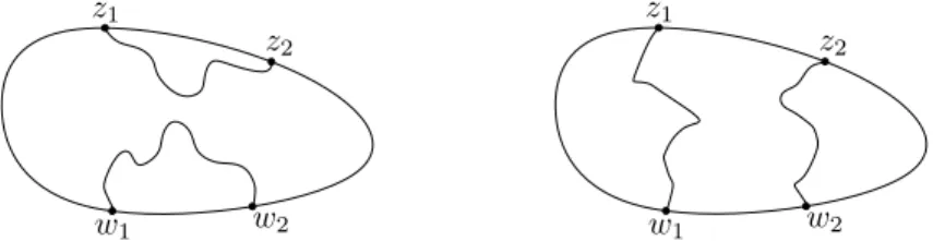
Bauer, Bernard, and Kyt¨ol¨a [4], there are two distinctarch-types that may result. We prefer to use the phrase type of configuration instead, and say that the resulting multiple interface
1No mathematical proof with all the details has been written down as of yet, although initial analysis
configuration is of either Type I if it joins w1 tow2 and z1 toz2, or of Type II if it joins z1
tow1 and z2 to w2; see Figure 1.
w1 w2
z1
z2
w1 w2
z1
z2
Figure 1: Configuration of Type I (left) and Type II (right).
In the language of conformal field theory, an interface is a non-local observable, and Arguin and Saint-Aubin [3] used CFT techniques to give a prediction for the probability of a configuration of Type II. They described the asymptotic behaviour of this probability using non-unitary representations that followed from the boundary scaling exponent h1,2 of
the Kac table.
Arguin and Saint-Aubin considered the Ising model at criticality on a half-infinite cylinder of radius 1. They represented the half-infinite cylinder by the unit disk D and denoted by
θj, j = 1, ..,4, the four points along the boundary where the spin flips occurred.
They then conformally mapped the unit disk to the upper half plane, and argued that the four point correlation function of the fieldφ =φ2,1 of conformal weight 12 is
hφ(z1), φ(w1), φ(z2), φ(w2)i=
1
(z1−w1)(z2−w2)
g
(z1−w1)(z2−w2)
(z1−z2)(w1−w2)
where g is a solution to the differential equation 3z(z−1)2g′′
(z) + 2(z−1)(z+ 1)g′
(z)−2zg(z) = 0. (7) This second order differential equation has two solutions—the first with exponent 0 and the second with exponent 53. Arguin and Saint-Aubin argued that the solution with exponent 53 corresponded to the probability of a configuration of Type II, and then found
P{config of Type II}= 1 2 −
9 20
Γ(1 3)
Γ(2
3)2f(0)(ξ)
f(5/3)(ξ)− ξ
1−ξf
(5/3)(1−ξ)
(8) with
f(0)(ξ) = 1−ξ+ ξ
1−ξ and f
(5/3)(ξ) = ξ5/3
1−ξF(−
1 3,
4 3,
8 3, ξ)
where F =2F1 denotes the hypergeometric function and
ξ= (z1−w1)(z2−w2) (z1−z2)(w1−w2)
denotes the cross-ratio. Furthermore, asξ →0, it follows that
P{config of Type II} ∼1− 10 9
Γ(2 3)
2
Γ(1 3)
ξ5/3+ O(ξ2).
6
Definition of a partition function for two paths and
a crossing probability calculation
Recall from Section 3 that HD,b,n(z,w) is defined to be the mass of the configurational
measure QD,b,n(z,w) and thatHD,b,n satisfies the scaling rule
HD,b,n(z,w) =|f
′
(z)|b|f′
(w)|bH
f(D),b,n(f(z), f(w)).
If we now define
˜
HD,b,n(z,w) =
HD,b,n(z,w)
HD,b,1(z1, w1)· · ·HD,b,1(zn, wn)
, (9)
then ˜HD,b,n(z,w) is a conformalinvariant. Thus, by conformal invariance, it suffices to work
in D=H.
In the case of two paths, an explicit calculation is possible and is given by the following proposition which has appeared in a number of places. It was first stated in a rigorous mathematical context by Dub´edat [8] using an infinitesmal approach, and was derived using CFT by Bauer, Bernard, and Kyt¨ol¨a [4]. A detailed derivation first appeared in [16]. As we will see shortly, the special case of the Ising model actually appeared earlier in Arguin and Saint-Aubin [3].
Proposition 6.1. Consider the upper half plane H, and let 0< x < y <∞. Ifb ≥ 1 4, then
˜
HH,b,2((0, x),(∞, y)) =
Γ(2a) Γ(6a−1) Γ(4a) Γ(4a−1)(x/y)
aF(2a,1
−2a,4a;x/y) (10)
where F =2F1 denotes the hypergeometric function and a= 2/κ= (2b+ 1)/3.
The proof of this proposition in [16] is accomplished by finding and then solving a differen-tial equation satisfied by ˜HH,b,2((0, x),(∞, y)). By scaling, we can write ˜HH,b,2((0, x),(∞, y)) =
ψ(x/y) for some functionψ =ψH,b of one variable. We then show that the ODE satisfied by
ψ is
u2(1−u)2ψ′′
(u) + 2u(a−u+ (1−a)u2)ψ′
(u)−a(3a−1)(1−u)2ψ(u) = 0
where a = 2/κ. In the particular case that κ = 3 so that a = 2
3, this differential equation
reduces to
3u2(1−u)ψ′′
(u) + 2u(2−u)ψ′
(u)−2(1−u)ψ(u) = 0.
If we change variables by setting g(z) = ψ(1−z), then g satisfies 3z(z−1)2g′′
(z) + 2 (z−1) (z+ 1)g′
(z)−2z g(z) = 0 which is exactly (7) above.
Remark. It is important to note that the restriction to b ≥ 1
4 is needed to guarantee that
0< κ ≤4. Formally, if we plug in κ = 6, then we recover Cardy’s formula for percolation; however, constructing a configurational measure on non-crossing SLE paths in the non-simple regime (4< κ < 8) is still an open problem.
We now explain how Proposition 6.1 can be used to calculate a crossing probability for two SLEκ paths (0 < κ ≤ 4). Choosing κ = 3 as a special case yields the desired
result of Arguin and Saint-Aubin [3], and of Bauer, Bernard, and Kyt¨ol¨a [4], for the critical Ising model. By conformal invariance, it is enough to work in the upper half plane H with boundary points 0, 1, ∞, and x where 0 < x < 1 is a real number. The possible interface configurations are therefore of two types, namely (I) a simple curve connecting 0 to ∞ and a simple curve connectingxto 1, or (II) a simple curve connecting 0 tox and a simple curve connecting 1 to ∞. The configurational measure corresponding to Type I is
QH,b,2((0, x),(∞,1))
and the configurational measure corresponding to Type II is
QH,b,2((x,1),(0,∞)).
By the symmetry of chordal SLE about the imaginary axis, however,
QH,b,2((x,1),(0,∞)) =QH,b,2((0,1−x),(∞,1)).
The partition function corresponding to a configuration of Type I is (defined as)
Zb,I(x) :=HH,b,2((0, x),(∞,1))
and the partition function corresponding to a configuration of Type II is (defined as)
Zb,II(x) := HH,b,2((0,1−x),(∞,1)) =Zb,I(1−x).
Therefore, the probabilities of a configuration of Type I and of a configuration of Type II are given by
Zb,I(x)
Zb,I(x) +Zb,II(x)
and Zb,II(x)
Zb,I(x) +Zb,II(x)
= Zb,I(1−x)
Zb,I(x) +Zb,II(x)
, (11) respectively.
Remark. As indicated in Section 3, we chose to normalize our kernel in such a way that
HH,b,1(0,∞) = 1. Thus, there is no arbitrary constant in our definition of either Zb,I(x) or
Zb,II(x). Suppose, however, that we had normalized our kernel differently, sayHH,b,1(0,∞) =
C for some C > 0. Although both Zb,I(x) and Zb,II(x) would now depend on C, the ratios
in (11) would not.
Remark. To be precise, the construction in Section 3 only defines the configurational measure for a given type of configuration. If we want to consider configurations without regard to type, then we need to define a measure supported on mutually-avoiding pairs of curves of either type. Of course, such a measure is given by the sum of the configurational measures of Types I and II, repectively. The mass of this measure is Zb,I(x) +Zb,II(x), and so the
probability measure on mutually-avoiding pairs of curves of either type is
P= QH,b,2((0, x),(∞,1)) +QH,b,2((x,1),(0,∞))
Zb,I(x) +Zb,II(x)
Thus, if Ais the event A={config of Type I}, then
P(A) = QH,b,2((0,x),(∞,1))(A)+QH,b,2((x,1),(0,∞))(A)
Zb,I(x)+Zb,II(x)
= Zb,I(x)+0
Zb,I(x)+Zb,II(x)
and, similarly, forP(Ac) = P{config of Type II}as in (11). We can now give a more careful
statement of the consequence of Smirnov’s work mentioned at the beginning of Section 5, namely that if PN denotes the probability measure for the two interfaces on the 1/N-scale
lattice, thenPN converges weakly to P.
Now by (4) and (9), we know that
HH,b,2((0, x),(∞,1)) =HH,b,1(0,∞)·HH,b,1(x,1)·H˜H,b,2((0, x),(∞,1))
= (1−x)−2b ˜
HH,b,2((0, x),(∞,1))
so that Proposition 6.1 yields
Zb,I(x) =HH,b,2((0, x),(∞,1)) =
Γ(2a) Γ(6a−1) Γ(4a) Γ(4a−1)x
a(1−x)−2b
F(2a,1−2a,4a;x).
Using (15.3.3) of [1], we can write
F(2a,1−2a,4a;x) = (1−x)4a−1
F(2a,6a−1,4a;x). (12) If we also note that a= 2/κ so that (3) implies 2b= (6−κ)/κ= 3a−1, then we can write
Zb,I(x) =
Γ(2a) Γ(6a−1) Γ(4a) Γ(4a−1)x
a(1
−x)aF(2a,6a−1,4a;x) and
Zb,II(x) =
Γ(2a) Γ(6a−1) Γ(4a) Γ(4a−1)x
a(1−x)aF(2a,6a−1,4a; 1−x).
Hence, we conclude from (11) that
P{config of Type I}= F(2a,6a−1,4a;x)
F(2a,6a−1,4a;x) +F(2a,6a−1,4a; 1−x) (13) and
P{config of Type II}= F(2a,6a−1,4a; 1−x)
F(2a,6a−1,4a;x) +F(2a,6a−1,4a; 1−x). (14)
7
Summary of results for the 2d critical Ising model
In the particular case of the 2d critical Ising model (in which case κ= 3), then (14) yields the probability of a configuration of Type II as follows:
P1(x) =
F(43,3,83; 1−x)
Using (15.3.3) of [1] (as in (12) above) Arguin and Saint-Aubin [3] express the same proba-bility (8) as
P2(x) =
1 2−
9 20
Γ(1 3)
Γ(2 3)2
x5/3(1−x)5/3
1−x+x2
F(4 3,3,
8
3;x)−F( 4 3,3,
8
3; 1−x)
whereas it is given in Bauer, Bernard, and Kyt¨ol¨a [4] as
P3(x) =
Z 1
0
y2/3(1−y)2/3
(1−y+y2)2 dy
−1Z 1
x
y2/3(1−y)2/3
(1−y+y2)2 dy.
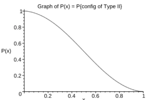
It is not at all obvious that these three expressions are identical. However, since all three represent the same physical observable (and since each was obtained by solving the same differential equation), it must be the case that P1(x) = P2(x) = P3(x) for 0 ≤ x ≤ 1; see
Figure 2.
Graph of P(x) = P{config of Type II}
0 0.2 0.4 0.6 0.8 1
P(x)
0.2 0.4 0.6 0.8 1 x
Figure 2: Graph ofP(x) =P1(x) =P2(x) =P3(x) for 0≤x≤1.
The easiest way to verify their equivalence is simply to check directly that each satisfies the required differential equation with the given boundary conditions. It is also possible to verify algebraically that these three expressions are the same by converting all of the hypergeometric functions into associated Legendre functions of the first kind.
Remark. The calculation ofP1(x) follows from SLE-techniques in a mathematically rigorous
way, and it provides an explanation for the results of Arguin and Saint-Aubin as well as Bauer, Bernard, and Kyt¨ol¨a. The key point is that the result of Smirnov tells us precisely what is meant by a scaling limit of the Ising model, namely the interface separating +1 spins from −1 spins viewed as a probability measure on curves converges weakly to the law of choral SLE3. Thus, by choosingκ= 3 we should be able to use SLE to recover results from
CFT for the Ising model such as the one that Arguin and Saint-Aubin derived.
8
Intersection probabilities for SLE
κ,
0
< κ
≤
4
, and a
Brownian excursion
The techniques that were used in [16] to derive Proposition 6.1 leads to a calculation of the probability that an SLE2 path and a Brownian excursion do not intersect. This was the
key in establishing the scaling limit of Fomin’s identity for loop-erased random walk [15]. In this section, we extend those ideas to compute the probability that an SLEκ path and a
Brownian excursion do not intersect. This event is illustrated in Figure 3.
0 x y
∞
γ[0,∞), a chordal SLEκ β[0, tβ], a Brownian excursion
Figure 3: Schematic representation of P{γ[0,∞)∩β[0, tβ] =∅}.
Theorem 8.1. Suppose that 0 < x < y <∞ are real numbers and let β : [0, tβ] →H be a
Brownian excursion from x to y in H. If γ : [0,∞)→H is a chordal SLEκ from 0 to ∞ in H, then
P{γ[0,∞)∩β[0, tβ] =∅ }=
Γ(2a)Γ(4a+ 1)
Γ(2a+ 2)Γ(4a−1)(x/y)F(2,1−2a,2a+ 2;x/y) (15)
where F =2F1 is the hypergeometric function and a= 2/κ.
Since the proof of this theorem is similar to the proof of Theorem 6.1 in [15], we omit many details.
Proof. Let Φ(x, y) =P{γ[0,∞)∩β[0, tβ] =∅}. Using Itˆo’s formula, it can be shown that Φ
satisfies the differential equation
−a 1 x − 1 y 2
Φ + a
x ∂Φ ∂x + a y ∂Φ ∂y + 1 2
∂2Φ
∂x2 +
1 2
∂2Φ
∂y2 +
∂2Φ
∂x∂y = 0. (16)
SLE scaling implies that the probability in question only depends on the ratio x/y, and so Φ(x, y) =ϕ(x/y) for some function ϕ=ϕH,b of one variable. Thus, we find
∂Φ
∂x =y
−1
ϕ′
(x/y), ∂Φ
∂y =−xy
−2
ϕ′
(x/y), ∂
2Φ
∂x2 =y
−2
ϕ′′ (x/y), ∂2Φ
∂y2 = 2xy
−3
ϕ′
(x/y) +x2y−4
ϕ′′
(x/y), ∂
2Φ
∂x∂y =−y
−2
ϕ′
(x/y)−xy−3
ϕ′′ (x/y),
so that after substituting into (16), multiplying byy2, lettingu=x/y, and combining terms,
we have
u2(1−u)ϕ′′
(u) + 2u(a+ (a−1)u)ϕ′
using the constraint 0 < u < 1. The second-order ordinary differential equation (17) has regular singular points at 0, 1, and ∞, and so we know that it is possible to transform it into a hypergeometric differential equation. By writing (17) as
ϕ′′ (u) +
2a u +
2−4a u−1
ϕ′
(u) +
2a u −2a
ϕ(u)
u(u−1) = 0 (18) we see that we have a case of Riemann’s differential equation whose complete set of solutions (see (15.6.1) and (15.6.3) of [1]) can be denoted by Riemann’s P-function
ϕ(u) =P
0 ∞ 1
1 −2a 4a−1 u
−2a 1 0
.
By now considering (15.6.11) of [1], the transformation formula for Riemann’sP-function for reduction to the hypergeometric function, we see that the appropriate change-of-variables to apply isψ(u) =u−1
(1−u)1−4a
ϕ(u) noting that this is permitted by the constraint 0< u <1. Thus, (17) implies
u(1−u)ψ′′
(u) + (2a+ 2−(6a+ 2)u)ψ′
(u)−2a(4a+ 1)ψ(u) = 0. (19) We see that (19) is now a well-known hypergeometric differential equation [1] whose general solution is given by
ψ(u) =C1F(2a,4a+ 1,2a+ 2;u) +C2u
−1−2a
F(−1,2a,−2a;u).
and so
ϕ(u) = u(1−u)4a−1
C1F(2a,4a+ 1,2a+ 2;u) +C2u
−1−2a
F(−1,2a,−2a;u) .
Using equation (15.3.3) of [1] we find
F(2a,4a+ 1,2a+ 2;u) = (1−u)1−4a
F(2,1−2a,2a+ 2;u) which implies that
ϕ(u) = C1u F(2,1−2a,2a+ 2;u) +C2u
−2a
(u−1)4a−1
F(−1,2a,−2a;u).
However, it follows immediately from the continuity of the Brownian excursion measure [14] and the fact that γ(0,∞)∩R=∅ when 0< κ≤4 that ϕ(u)→0 as u→0+ andϕ(u)→1 as u→1−. This implies C2 = 0 and
C−1
1 =F(2,1−2a,2a+ 2; 1) = lim
u→1−F(2,1−2a,2a+ 2;u) =
Γ(2a+ 2)Γ(4a−1) Γ(2a)Γ(4a+ 1) . Thus,
ϕ(u) = Γ(2a)Γ(4a+ 1)
Γ(2a+ 2)Γ(4a−1)u F(2,1−2a,2a+ 2;u) and so (15) follows as required.
Remark. Theorem 8.1 provides another example of an SLE observable. Hence, the primary application of Theorem 8.1 to a physical situation seems to be as a way to provide evi-dence that a particular statistical mechanics lattice model interface has an SLE limit. A conjectured value of κ may be found, or verified, by approximating the probability that a Brownian excursion and an interface intersect, and then comparing the result to that given in this theorem. In order to actually do this numerically, however, there are a number of issues with which one must contend. These include selecting a lattice with which to work, defining and then simulating an appropriate interface, and then simulating a simple random walk excursion on the lattice (since simple random walk excursions converge to Brownian excursions; see [14], for instance).
As an example where the observable from this theorem might be applied, consider the recent work of Bernard, Le Doussal, and Middleton [6]. They perform several statistical tests of the hypothesis that zero-temperature Ising spin glass domain walls are described by an SLEκ, and working on the triangular lattice they find numerically these domain walls to
be consistent with κ = 2.32±0.08. Among the observables studied in [6] that led to this conclusion is the SLE left-passage probability (which, incidentally, is also given in terms of a hypergeometric function). The work of Bernard, Le Doussal, and Middleton extends earlier work of Amoruso, Hartmann, Hastings, and Moore [2] who presented numerical evidence that the techniques of CFT might be applicable to two-dimensional Ising spin glasses, and that such domain walls might be described by a suitable SLE. In particular, the observable studied in [2] was the fractal dimension of the domain walls.
The transition probabilities for simple random walk excursions on the triangular lattice can be computed. This means that such random walks can be simulated, and so it seems possible that the numerical techniques used in either [6] or [2] could actually be applied for the observable of Theorem 8.1.
9
Conclusion
The construction of the configurational measure on n-tuples of mutually avoiding, simple SLE paths by Kozdron and Lawler [16] leads to a possible definition of a partition function for SLE. Using this definition, a mathematically rigorous proof can be given for certain theoretical predictions about the 2d critical Ising model that Arguin and Saint-Aubin [3] originally derived using only CFT techniques (i.e., no SLE mentioned in their work). As well, this gives a mathematically rigorous derivation of the general results of Bauer, Bernard, and Kyt¨ol¨a [4] concerning crossing probabilities for two interfaces in the simple (0< κ≤4) regime that they derived previously using CFT techniques. It also leads to the calculation of the probability that an SLEκ path (with 0 < κ ≤ 4) and a Brownian excursion do not
intersect.
Acknowledgements
This paper had its origin at the Workshop on Stochastic Loewner Evolution and Scaling Limits held in August 2008 at the Centre de Recherches Math´ematiques. Thanks are owed
to Yvan Saint-Aubin who brought the work [3] to the attention of the author, as well as to the Natural Sciences and Engineering Research Council (NSERC) for providing financial support through the Discovery Grant program.
References
[1] M. Abramowitz and I. A. Stegun, editors. Handbook of Mathematical Functions with Formulas, Graphs, and Mathematical Tables. National Bureau of Standards, Washing-ton, DC, 1972.
[2] C. Amoruso, A. K. Hartmann, M. B. Hastings, and M. A. Moore. Conformal Invariance and Stochastic Loewner Evolution Processes in Two-Dimensional Ising Spin Glasses.
Phys. Rev. Lett., 97:267202, 2006.
[3] L.-P. Arguin and Y. Saint-Aubin. Non-unitary observables in the 2d critical Ising model.
Phys. Lett. B, 541:384–389, 2002.
[4] M. Bauer, D. Bernard, and K. Kyt¨ol¨a. Multiple Schramm-Loewner Evolutions and Statistical Mechanics Martingales. J. Stat. Phys., 120:1125–1163, 2005.
[5] M. Bauer and D. Bernard. 2D growth processes: SLE and Loewner chains. Phys. Rep., 432:115–221, 2006.
[6] D. Bernard, P. Le Doussal, and A. A. Middleton. Possible description of domain walls in two-dimensional spin glasses by stochastic Loewner evolutions. Phys. Rev. B, 76:020403(R), 2007.
[7] J. Cardy. SLE for theoretical physicists. Ann. Phys., 318:81–118, 2005.
[8] J. Dubedat. Euler integrals for commuting SLEs. J. Stat. Phys., 123:1183–1218, 2006. [9] J. Dub´edat. SLE and the free field: Partition functions and couplings. Preprint, 2007. [10] B. Duplantier and S. Sheffield. Liouville quantum gravity and KPZ. Preprint, 2008. [11] R. Friedrich and W. Werner. Conformal restriction, highest-weight representations and
SLE. Comm. Math. Phys., 243:105–122, 2003.
[12] I. Gruzberg. Stochastic geometry of critical curves, Schramm-Loewner evolutions and conformal field theory. J. Phys. A, 39:12601–12655, 2006.
[13] W. Kager and B. Nienhuis. A guide to stochastic Loewner evolution and its applications.
J. Statist. Phys., 115:1149–1229, 2004.
[14] M. J. Kozdron. On the scaling limit of simple random walk excursion measure in the plane. ALEA Lat. Am. J. Probab. Math. Stat., 2:125–155, 2006.
[15] M. J. Kozdron. The scaling limit of Fomin’s identity for two paths in the plane. C.R. Math. Rep. Acad. Sci. Canada, 29:65–80, 2007.
[16] M. J. Kozdron and G. F. Lawler. The configurational measure on mutually avoiding SLE paths. In I. Binder and D. Kreimer, editors, Universality and Renormalization: From Stochastic Evolution to Renormalization of Quantum Fields, Volume 50 ofFields Institute Communications, pages 199–224, American Mathematical Society, Providence, RI, 2007.
[17] K. Kyt¨ol¨a. Virasoro Module Structure of Local Martingales of SLE Variants.Rev. Math. Phys., 19:455–509, 2006.
[18] G. F. Lawler. Conformally Invariant Processes in the Plane. American Mathematical Society, Providence, RI, 2005.
[19] G. F. Lawler. Partition functions, loop measures, and versions of SLE. Preprint, 2008. [20] G. F. Lawler and W. Werner. The Brownian loop soup. Probab. Theory Related Fields,
128:565–588, 2004.
[21] O. Schramm. Scaling limits of loop-erased random walks and uniform spanning trees.
Israel J. Math., 118:221–288, 2000.
[22] S. Smirnov. Towards conformal invariance of 2D lattice models. In M. Sanz-Sol´e, J. So-ria, J. L. Varona, and J. Verdera, editors, Proceedings of the International Congress of Mathematicians, Madrid, Spain, 2006. Volume II, pages 1421–1451, European Mathe-matical Society, Zurich, Switzerland, 2006.
[23] S. Smirnov. Conformal invariance in random cluster models. I. Holomorphic fermions in the Ising model. To appear, Ann. Math.
[24] W. Werner. Random planar curves and Schramm-Loewner evolutions. In Lectures on Probability Theory and Statistics: Ecole d’Et´e de Probabilit´es de Saint-Flour XXXII-2002, volume 1840 of Lecture Notes in Mathematics, pages 107–195. Springer-Verlag, Berlin, 2004.
![Figure 3: Schematic representation of P {γ[0, ∞) ∩ β[0, t β ] = ∅}.](https://thumb-us.123doks.com/thumbv2/123dok_us/8557958.2312758/13.918.280.650.187.359/figure-schematic-representation-p-γ-β-t-β.webp)
