Multiple Regression Used in Macro-economic Analysis

(1)

Multiple Regression Used in Macro-economic

Analysis

Prof. Constantin ANGHELACHE PhD

„Artifex” University of Bucharest /

Academy of Economic Studies, Bucharest

Prof. Mario G.R. PAGLIACCI PhD

Universita degli Studi di Perugia

Assoc. prof. Elena BUGUDUI PhD

„Artifex” University of Bucharest

Assistant teacher Ligia PRODAN PhD Student

„Dimitrie Cantemir” Christian University, Bucharest

Ec. Bogdan DRAGOMIR

Abstract

GDP, one of the main macroeconomic aggregates specific to SNA

represents the synthetic expression of economic activity results produced

within the economic territory over a period of time, regardless of the

contribution that they had domestic or foreign subjects.

Key words:

aggregate, multiple regression, correlation, residual,

regressor

JEL Classification:

C22, C25

The economic situation in which correlations involves only two variables are very rare. Rather we have a situation where a dependent variable, Y, can depend on a whole series of variables factorial or regressor. In practice, there are correlations of the form:

Y = β1 + β2 X2 + β3X3 + β4X4 +...+ βkXk + ε

where values Xj (j = 2, 3, ..., n) represents the variable factor or regressors, the

values βj (j = 1, 2, 3, ...,k) are the regression parameters, and ε is the residual factor

factor.

Residual factor reflects the random nature of human response and any other factors, others than Xj, which might influence the variable Y.

We adopted the usual notation, respectively assigned to the first factor notation X2, the second notation X3 and so on. Sometimes it is convenient that the

parameter β to be considered that coefficient of one variable X1 whose value is

always equal to unity. Then the relationship is rewritten as:

(2)

In the case of regression with two variables (E(ε) = 0), then, substituting, for given values of the variables X, we get:

E(Y)=β1 + β2 X2 + β3X3 + β4X4 +...+ βkXk

The relationship is multiple regression equation1_{. For now, conventional,}

we consider that it is the linear form. Unlike the case of two-variable regression, we can not represent this equation in a two-dimensional diagram. βJ are regression

parameters. Sometimes, they are also called regression coefficients. β1 is a constant

(intercept) and β2 , β3 and so on, are the regression slope parameters.

β4, measuring the effects of E(Y) produced by changing one unit of X4,considering

that all other factor variables remain constant. β2 measures the effects on E(Y)

produced by changing one unit of X2, considering that all other variables remain

constant factor.

As the population regression equation is unknown, it hase to be estimated based on data sample. Suppose that we have available a sample of n observations, each observation containing the dependent variable values for both Y and for each factorial variables X. We write the values for observation i as:

Yi , X2i , X3i , X4i ,..., Xki

For example, X37 is the value of X3 in the 7 th observation and X24is the

value X2 taken in the 4 th observation. For a similar manner, Y6 is the variable Y in

the observation of 6 and so on.

Given that it is assumed that the sample data were generated by the correlation of the population, each observation have to involve a set of values satisfy the multiple ecuation regression.

We can write the equation:

Yi = β1 + β2X2i +β3X3i + ...+ βkXki + εi for all the values,

where εi represents the residual value for the observation of the i.

We can rewrite the relationship in a simple matrix form, as follows:

Y = Xβ + ε , where

X is a matrix the form of n x k with k column of values and then all sample values of the k – 1, X variables.

Thus, the fourth column of X, for example, contains the values of X4 of the

sample n, the seventh column contains the values of X7 and so on. β is a vector of k

x 1 column containing the parameters βj and ε is an vector of n x 1 column

containing the residual values.

The effective values of Y will not coincide with the expected values of Y

and, in the case of two-variable regression, the differences between them are known as residual values.

Like Yi =Yi+ei

^

for all values of i

(3)

where ei is the residual corresponding to the observations of i.

The relationship can be written as:

Yi = + X i + X i + + ki Xki +ei

^ 3 3 ^ 2 ^ 2 1 ^ ...

β

_{, for all values of}_i_{or on matrix}

form:

e X

Y =

β

^+ _,_where_X_and_Y_{are already defined}

There are two issues to be retained on the residual values.

First, regardless of the method used to estimate the regression equation, we get such residual values - one for each of the sample observations. Second, as

expected j

^

β

when it becomes known and can be used to calculate them. Now, we need to calculate the differential with the vector

^

β

_{and equalizer}

to zero the result. Such of this matrix lead to the following relation:

0 '

2 '

2

^ ^

=

−

+

=

∂

_β

β

X

Y

X

S

The above equation is a set of k equations that can be written as:

Y X X

X'

β

^ = '

Example:

In the analysis of the factors that determine the variation of GDP, we started from specific compenent elements of using the final production method (expenditure method), considering that this is a significant source of information on the main correlations that influence the evolution of the main macroeconomic aggregate.

Thus, according to the calculation method above, GDP involves adding components that express using of goods and services for final production, as follows:

PIB = CF + FBC + EXN

Based on the elements mentioned above we want to identify the existing relationship between the evolution of the country's final consumption (regarded as a sum of private and public consumption), net investment and GDP variation.

In this regard, we used linear multiple regression analysis as a method in which we consider GDP as outcome variables and the variable factor the final consumption value and net investments in our country during 1998-2011.

(4)

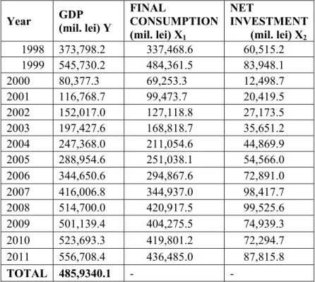
Table 1 Evolution of GDP, final consumption and net investment in Romania during 1998-2011

Year GDP _{(mil. lei) Y}

FINAL

CONSUMPTION (mil. lei) X1

NET

INVESTMENT (mil. lei) X2

1998 373,798.2 337,468.6 60,515.2 1999 545,730.2 484,361.5 83,948.1 2000 80,377.3 69,253.3 12,498.7 2001 116,768.7 99,473.7 20,419.5 2002 152,017.0 127,118.8 27,173.5 2003 197,427.6 168,818.7 35,651.2 2004 247,368.0 211,054.6 44,869.9 2005 288,954.6 251,038.1 54,566.0 2006 344,650.6 294,867.6 72,891.0 2007 416,006.8 344,937.0 98,417.7 2008 514,700.0 420,917.5 99,525.6 2009 501,139.4 404,275.5 74,939.3 2010 523,693.3 419,801.2 72,294.7 2011 556,708.4 436,485.0 87,815.8

TOTAL 485,9340.1 - -

Source: Statistical Yearbook of Romania, Gross Domestic Product, categories of uses, NIS, Bucharest, 2008, 2009, 2010, 2011, 2012

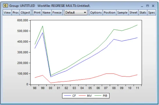
For an pertinent analyze of the correlation between the three macroeconomic indicators presented in the table above, it is necessary in a first step of this research to identifie a number of features aiming the evolution of each indicator considered in the period under review. To prove this, using the software Eviews 7.2, we studied in the first stage, the evolution of the three indicators.

As can be seen from analyzing the data series under investigation, especially as in the figure shown above, in the period considered,the three of our country's macroeconomic indicators have registered a steady growth from year to year, except to this rule making 2000 and 2009 when there was a decrease of the three indicators.

The purpose of multiple regression (term used by Pearson, 1908) is to highlight the relationship between a dependent variable (explained endogenous effect) and a lot of independent variables (explanatory factors, exogenous predictors).

(5)

Figure 1. Evolution of GDP, final consumption and net investment in Romania in the period 1998 - 2011

Multiple linear regression model equation will look like this: Y=b0+b1X1+b2X2+

ε

in which:

Y - Gross Domestic Product- GDP; X1 - Final Consumption- CF;

X2 -Net investments- INV;

b0,b1,b2 - parameters of the regression model;

ε

is a variable, interpreted as error (disturbance, measurement error).

The regression model may be rewrite under the following mathematical equation: PIB= b0+b1CF+b2INV+

ε

To estimate the regression model parameters we used the software Eiews 7.2 in which we defined an equation that has as outcome variables GDP, and factor variables the final consumption and net investments.We also thought that this regression model will also include free term c, which is expected to influence dimming terms that were not taken into account when we building this model. Estimation method defined in the program is the method of least square.

(6)

Figure 2. Characteristics of the regression model

From the above, multiple regression model describing the relationship between the three macroeconomic indicators that are are the subject of previously determined may be given in the form of equation as follows:

PIB = -8.927,569 + 1,165488 CF + 0,284958 INV

Thus, we can say that an increasing with a monetary unit of final consumption (with its two compenent - private consumption and public consumption) will lead to an increase of 1.165488 units monetary of gross domestic product value. In case of the net investment, the difference is more significant, we can see that every leu invested brings an increase of only 0.284958 lei of the level of gross domestic product. This situation correspondes with the reality economics of Romania because in the last twenty years the Romanian economy was based almost exclusively on stimulating consumption and less on promotion of an investment policy correctly.

The influence of the free term as a picture of the factors that were not included in the analysis model is one significant. In fact, it can be said, that the factors that were not included in the econometric model of analysis, they have an significant decrease in the value of gross domestic product.

(7)

Also the validity of the regression model is confirmed by the F test value - statistically superior value table level that is considered to be the benchmark in the analysis of the validity of econometric models and by the value of the test Prob (F - statistic) that it is zero.

Based on observations made on the analysis of Romania's GDP, using multiple regression model, we conclude that the value of this indicator is significantly influenced by the variation of final consumption and net investment less variation.

Using a multifactorial regression model allows to obtain more edifying results in macroeconomic analysis and conducting relevant research on the evolution of the national economy.

References

Anghelache, C. şi alţii (2012) – „Elemente de econometrie teoretică şi aplicată”, Editura Artifex, Bucureşti

Anghelache, C., Mitruţ, C. (coordonatori), Bugudui, E., Deatcu, C. (2009) – „Econometrie: studii teoretice şi practice”, Editura Artifex, Bucureşti

Bardsen, G., Nymagen, R., Jansen, E. (2005) – „The Econometrics of Macroeconomic Modelling”, Oxford University Press

Benjamin, C., Herrard, N., Houée-Bigot, M., Tavéra, C. (2010) – „Forecasting with an Econometric Model”, Springer

Dougherty, C. (2008) – “Introduction to econometrics. Fourth edition”, Oxford University Press

Gourieroux, C., Jasiak, J. (2001) – „Financial econometrics: problems, models and methods”, Princeton University Press, Princeton

Hendry, D.F. (2002) – „Applied econometrics without sinning”, Journal of Economic Surveys, 16

Jesus Fernandez-Villaverde & Juan Rubio-Ramirez (2009) – “Two Books on the New Macroeconometrics”, Taylor and Francis Journals, Econometric Reviews Mario G.R. Pagliacci, Gabriela Victoria Anghelache,Ioana Mihaela Pocan, Radu

Titus Marinescu, Alexandru Manole “Multiple Regression – Method of

Financial Performance Evaluation”, ART ECO – Review of Economic

Studies and Research, Editura Artifex, Vol. 2/No.4/2011, pp. 3-9.

Mitruţ, C. (2008) – „Basic econometrics for business administration”, Editura ASE, Bucureşti

Voineagu, V., Ţiţan, E. şi colectiv (2007) – “Teorie şi practică econometrică”, Editura Meteor Press