arXiv:2101.02015v1 [quant-ph] 6 Jan 2021
Avoided level crossings in polynomial potentials
with
N
thick barriers
Miloslav Znojil
The Czech Academy of Sciences, Nuclear Physics Institute, Hlavn´ı 130, 250 68 ˇReˇz, Czech Republic
and
Department of Physics, Faculty of Science, University of Hradec Kr´alov´e, Rokitansk´eho 62, 50003 Hradec Kr´alov´e, Czech Republic
e-mail: [email protected] and
Denis I. Borisov
Institute of Mathematics, Ufa Federal Research Center, RAS, Chernyshevskii str. 112, 450008 Ufa, Russia
and
Bashkir State University, Zaki Validi str. 32, 450076 Ufa, Russia and
Department of Physics, Faculty of Science, University of Hradec Kr´alov´e, Rokitansk´eho 62, 50003 Hradec Kr´alov´e, Czech Republic
e-mail: [email protected]
Keywords:
Schr¨odinger equation; multi-barrier polynomial potentials; avoided energy-level crossings; abrupt wavefunction re-localizations; quantum theory of catastrophes;
PACS number:
Abstract
A family of one-dimensional Schr¨odinger equations is considered, with the multi-well polynomial potentials characterized by anN−plet of the high and thick barriers separating the (N+1)−plet of the deep confining valleys. It is shown how the approximate low-lying spectra can be constructed participating in the tunneling-controlled fine-tuned competition of these valleys for the ground- or excited-state dominance and stability. These phenomena are interpreted as a quantum avoided-level-crossing analogue of the bifurcations of the long-time equilibria (also known, as Thom’s catastrophes) in classical dynamical systems.
1
Introduction
In many realistic applications of quantum mechanics (say, in molecular or nuclear physics) the structure of the bound-state spectrum is often found fairly sensitive to the variation of parameters. In particular, after a small change of these parameters some of the neighboring energy levels appear to merge and cross [1]. This happens in spite of the absence of any symmetry and in an apparent contradiction to the Hermiticity of the Hamiltonian. Although a more detailed inspection of the spectrum reveals that the crossings are in fact avoided, the phenomenon permanently attracts interest of theoreticians [2, 3, 4] as well as experimentalists [5]. One of the reasons is that after an analytic continuation of the Hamiltonian in the complex plane of a parameter, the avoided energy-level crossing (ALC) phenomenon proves intimately related to the complex singularities called (Kato’s) exceptional points (EPs, [6]).
In the one-dimensional Schr¨odinger equation
H(a, b, . . .)ψn(x) =En(a, b, . . .)ψn(x), n = 0,1, . . . , (1) H(a, b, . . .) =−~ 2 2µ d2 dx2 +V(x, a, b, . . .), ψn(x) ∈ L 2(−∞,∞)
an explicit form of the ALC-EP correspondence emerges even after the most elementary choice of the exactly solvable harmonic-oscillator potential [7]. One of the messages deduced from this observation is that whenever one studies the quantum ALC phenomenon, it makes sense to start the analysis from analytic potentials of polynomial form.
In our recent study [8] of Schr¨odinger equation (1) we paid attention to specific sequence of spatially symmetric polynomial potentials
V(3)(cusp)(x, c1) =x4 +c1x2, V(5)(butterf ly)(x, c1, c2) =x6+c1x4 +c2x2, . . . . (2)
This enabled us to find another analogy connecting the quantum ALC instants with the points of bifurcation of the long-term equilibria in certain classical dynamical systems. From the latter point of view the first two items of the list (2) play a key role also in the Thom’s classical catastrophe theory [9, 10]. The catastrophes represented by these benchmark potentials (also known, in non-quantum context, as Lyapunov functions) were even given the characteristic nicknames mentioned here in the superscripts.
Sequence (2) is just an even-parity subset of the general polynomial-potential family
V((kArnold) )(x, a, b, . . .) =xk+1+a xk−1
+b xk−2
+. . . , k= 1,2, . . . . (3) In an extended version of the Thom’s theory Arnold [11] offered a geometric picture of the branch-ing of evolutions in a generic one-dimensional dynamical system. He used the infinite family (3)
as benchmark models, and he showed why it represents the most natural k >5 classical-systems generalization of the Thom’s list.
In paper [8] it has been pointed out that at the odd subscripts k = 2N + 1 the classical catastrophes could be also paralleled, in consistent manner, by their quantized analogues. Under the assumption of spatial symmetry (2) such a project proved technically feasible. Via a suitable
ad hoc reparametrization of the couplings in (3), a systematic classification of the sudden ALC-related changes of the state of the systems has been obtained.
Naturally, due to the characteristic mathematical fact of the tunneling, not all of the classical types of the catastrophe found their fully analogous quantum counterpart. Some of them (like, e.g., cusp) got smeared out and smoothed after quantization. What still survived were the abrupt, catastrophe-like changes of the topological properties of probability densities. They remained measurable and, hence, phenomenologically meaningful. For this reason it has been suggested to call these specific types of the ALC-related bifurcations of equilibria “quantum relocalization catastrophes” (QRC).
In our present paper we intend to complement these results by a few vital and important addenda. First of all we will turn attention to the popular opinion (shared also in [8]) that the only meaningful form of quantization would be a transition from the study of minima of the Lyapunov functions (representing the stable long-term equilibria of classical systems) to the analogous analysis of the long-term stability of quantum ground states. We will point out that in such a most conventional approach it is usually tacitly supposed that in a way paralleling the behavior of classical systems one can ignore the excited states because their long-term stability is always destroyed by random perturbations.
Recently, such a mainstream philosophy has been criticized by Smilga [12]. He proposed that in any phenomenologically responsible analysis of the long-term stability of the excited states we always have to distinguish between the “malign” (i.e., the de-excitation supporting) and “benign” (i.e., the de-excitation not supporting) nature of the existing perturbations. This means that the stability status of the quantum excited states is always model-dependent. In other words, the conventional emphasis upon the destructive role of perturbations should not be exaggerated, especially in the most common case of the low-lying spectra of bound states which are often, in real world, all long-time stable. In this spirit we intend to demonstrate here the technical feasibility of an extension of the ALC-related constructions from the exclusive ground-state scenarios of Ref. [8] to the whole low-lying spectra of bound states (cf., in particular, section 3).
Secondly, besides such an extension of physics represented by the theory we will reconsider, in subsequent sections, also the fairly challenging mathematical problem of an enormous growth of the technical obstacles encountered after one removes the parity-symmetry constraint V(x) =V(−x)
as imposed by Eq. (2). Tentatively, a resolution of the challenge will be sought in a specific form of application of perturbation theory in which we will decompose the general Arnold’s confining quantum potential (4) into a dominant, even-parity unperturbed component V(even)(x) and an
odd-parity perturbation V(odd)(x).
Our basic idea will lie in a combination of the standard assumption of the smallness of per-turbations, V(odd)(x) =O(ǫ), with an innovative “re-use” of the above-mentioned technical
user-friendliness of the reparametrizations of the even-parity polynomials. Such a reparametrization of coefficients proved essential, in [8], during the localizations of ALCs for the Arnold’s polyno-mial potentials V(even)(x) = V(even)
(N) (x) of degree 2N + 2. Here, it will be applied to products
V(odd)(x) =ǫ x V(even)
(M) (x) in which the auxiliary factorization will transfer the control of the shape
ofV(odd)(x) to the control of the shape of the auxiliary even-parity polynomial of a smaller degree
2M + 2<2N + 2. In this manner, the repeated application of the same reparametrization trick to perturbations of an independently tunable shape will be shown equally efficient.
In the last section 6 our results will be, more thoroughly, discussed and summarized.
2
Relocalizations of ground states
2.1
The phenomenon of tunneling and its consequences
In phenomenological applications the choice of the potential in Schr¨odinger equation (1) is usually dictated by an expected correspondence between quantum system and its suitable classical-physics analogue. Such a purely intuitive idea played an important role not only during the birth of quantum mechanics but also in the various related methodical considerations. In paper [8], in particular, the classical-quantum correspondence has been found inspiring due to its relevance in dynamical systems. On the classical-physics side, the key role has been known to be played by the singular evolution scenarios called catastrophes [10] and/or bifurcations [13]. On the quantum theory side, unfortunately, the singularities of such a type are usually assumed “smeared out” by the quantization [14]. For this reason the progress in this field is far from rapid [15].
Incidentally, the range of applicability of the Thom’s qualitative picture of evolution patterns was by far not restricted to physics. In fact, the basic motivation of the development of the catastrophe-related mathematics lied, originally, in biology [9]. Moreover, its intuitive geometric form found, paradoxically, various formal and descriptive applications not only in disciplines like theoretical chemistry [16] but even in quantum physics itself [17, 18, 19].
Obviously, the deep conceptual differences between the classical and quantum pictures of reality are reflected also in the underlying mathematics. The necessity of replacement of the observed
numbers (representing, say, an energy or position of a classical point particle) by the operators in Hilbert space implies that the traditional variational and/or geometric tractability of these observables is lost, and the tools of the functional analysis have to be used [15]. Moreover, as we already mentioned, even the Arnold’s polynomial potentials (3) will lose their quantum-mechanical applicability at the odd subscripts k = 2N + 1. Thus, we have to restrict our attention to the subset of polynomials
V(x) =x2N+2+a x2N +b x2N−1
+. . .+z x (4) where an elementary shift of the origin on the real line ofxenabled us to eliminate the subdominant term. Without any loss of generality we were also able to fixV(0) via a suitable shift of the energy scale.
In the framework of classical theory our confining 2N−parametric potentials (4) can be char-acterized, according to Arnold [20], by the Dynkin diagrams Ak with odd k = 2N + 1. After
quantization, i.e., after insertion in Schr¨odinger equation (1) one could have a tendency to start from the two-parametricN = 1 model representing a classical catastrophic scenario called cusp,
V(x) =V(cusp)(a, b, x) =x4+a x2+b x . (5) Unfortunately, one merely reveals that also such a choice is to be excluded. Indeed, in contrast to the classical case, the solutions change smoothly with the parameters. The related classical cusp catastrophe proves really smeared out by the quantization [8]. Indeed, due to the phenomenon called quantum tunneling the wave function of the system will reside, even in double-well case, in both of the valleys. Hence, the change of the sign of a will not induce any abrupt changes of the observable features of the system.
After we incorporate the second variable coupling b, the left-right symmetry becomes broken, but the smoothness of the dynamics remains unchanged. The change ofbmerely moves one of the minima downwards. Locally, the well in its vicinity gets broadened so that irrespectively of the sign of b the other minimum moves up and, from the point of view of the low-lying spectrum, it loses its relevance. The ground-state wave function ψ0(x) will tunnel out of the upper well. The
process remains smooth. In a search for abrupt changes our attention has to be redirected to the less elementary shapes of potentials (4) with N ≥2.
2.2
The emergence of topology-changing quantum catastrophes at
N
= 2
Schr¨odinger equation −Λ2 d 2 dx2 +V (butterf ly))(x) ψn(x) =Enψn(x), Λ2 =~2/(2µ), n = 0,1, . . . (6)with the four-parametric potential
V(butterf ly)(x) =x6+a x4+b x3+c x2 +d x (7) is simpler to solve in its spatially symmetric version whereb=d= 0. The basic technical aspects of such a special case were discussed in [8]. In a slightly different notation let us now summarize these results briefly. First, in the spirit ofloc. cit., potential
V(x) =x6+a x4+c x2 (8) will only be considered here in its most interesting deep-triple-well dynamical regime. Under this assumption, the first derivative of the potential can be factorized in terms of the coordinates of the extremes of V(x) or, in other words, in terms of suitable realα and β,
V′ (x) = 6x5 + 4a x3+ 2c x= 6x(x4+ 4a 6 x 2 +2c 6 x) = 6x(x 2 −α2) (x2−α2−β2), (9) This induces a reparametrization of the original couplings,
a=a(α, β) = −3 (α2+β2/2), c=c(α, β) = 3α2(α2+β2). (10) The pronounced, deeply triple-well shape of the potential possessing two high and thick inner barriers will be achieved when and only when the coordinates of the extremes are chosen sufficiently large,α2 ≫Λ2 and β2 ≫Λ2. Thus, in units such that Λ2 = 1 we have to have α≫1 and β ≫1.
The latter, phenomenologically motivated assumption simplifies the approximate construction of bound states. Indeed, in the case of the dominance of the central attraction the approximate low-lying spectrum will acquire the elementary leading-order form
En(central) = (2n+ 1)pc(α, β) + higher order corrections, n = 0,1, . . . . (11)
The alternative assumption of the dominance of the off-central attraction yields the almost de-generate energy-level doublets
Em(even/odd) =V(pα2+β2) + (2m+ 1) Ω + higher order corrections, m = 0,1, . . . , (12)
Ω = q
V′′(pα2+β2)/2, V′′(pα2+β2) = 12α2β2+ 12β4
which are, naturally, never strictly degenerate.
As long as we haveV(pα2+β2) =α6+ 3/2α4β2−1/2β6 the ground-state version of formula
(12) reads
E0(even/odd)=α6+ 3/2α4β2−1/2β6+
p
Next, we will set β2 =µ2α2 with, say, µ=O(1). Asymptotically (i.e., in the regime of very large
parameters α ≫ 1 and β ≫ 1) we then deduce, from formula (11), that En(central) = O(α2). In
contrast, Eq. (13) implies thatEm(even/odd) =O(α6). This comparison reveals the clearly dominant
behavior of the off-central minimum of the potential. In the leading-order approximation the “quantum-catastrophic” instant of transition between the central and off-central dominance of the probability density of the ground states will be merely dictated by the trivial constraint
V(pα2+β2) = O(α2), i.e., up to corrections, by the elementary equation V(p
α2+β2) = 0.
This enables us to deduce that the quantum relocalization catastrophe becomes controlled by β
and realized atµ2 ≈µ
∞= 2, i.e., along the line ofβ ≈
√
2α. Only in the next order approximation one has to impose the explicit ALC condition
E0(central)(α, β) =E
(even/odd)
0 (α, β) + small corrections. (14)
The detailed analysis of its solutions may be found in [8].
3
Relocalization catastrophes involving excited states
The latter conclusion concerning the existence of the ground-state relocalization transitions fully agrees with the same result which was presented in Ref. [8] - one only has to keep in mind that in loc. cit. the meaning of the letter β was different. During a detailed analysis of the role of corrections one reveals that the assumption of the pronounced form of the minima and maxima of the potential (i.e., the work withα≫1 andβ ≫1) could also open a way towards an identification of a multitude of innovative “quantum-catastrophic” relocalization transitions to, and/or between, the various low-lying excited states.
In a concise explanation of the existence of a new class of the observable critical phenomena we should point out that in the deep-triple-well regime the level spacingsp
c(α, β)∼E0(cental) =O(α2)
and Ω(α, β) ∼ E0(even/odd) −V(p
α2+β2) = O(α2) are subdominant but still large. Thus, also
the excited states can still be well identified experimentally. In the language of the relocalization theory, its above-outlined ground-state version admits an immediate and meaningful upgrade, therefore. Eq. (14) becomes complemented by a natural low-lying-state-matching extension
Em(even/odd)(α, β) =En(central)(α, β) + small corrections, m, n= 0,1, . . . , Mmax. (15)
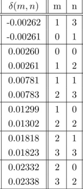
At every pair ofm andn the (necessarily, numerical) search for the solutions remains straightfor-ward. Table 1 offers an illustrative sample of these solutions at α= 4.
What one immediately notices is the smallness of the deviationsδ =δ(m, n) of the numerically evaluated critical ratios µ2 = β2/α2 from their unique asymptotic value µ2
Table 1: Numerical localization of bifurcations Em(even/odd)(α, β) = En(central)(α, β) at the critical
shifts δ =δ(m, n) using fixed α = 4 and variable β =µ α with growing µ=√2 +δ.
δ(m, n) m n -0.00262 1 3 -0.00261 0 1 0.00260 0 0 0.00261 1 2 0.00781 1 1 0.00783 2 3 0.01299 1 0 0.01302 2 2 0.01818 2 1 0.01823 3 3 0.02332 2 0 0.02338 3 2
this smallness is easily explained by the proportionality of the off-central energy values to the local bottomV(pα2+β2) of the potential. The decrease of this minimum is dictated by its very
large component −β6/2 so that the shift δ itself must remain small. From the point of view of
experimentalists, the high sensitivity of the process of the relocalization of the probability density to a parameter should be interpreted as an abrupt change of the topology of the system near a critical δ = δ(m, n). Hence, it makes sense to speak about the phenomenon of a quantum relocalization catastrophe even when the excited states are concerned.
The second striking feature of the excitation-dependent relocalization catastrophes which occur at the m− and n− dependent parameters µ = µ∞+δ(m, n) may be seen, in Table 1, in their
approximate pairwise degeneracy, with δ(1,3) ≈ δ(0,1), etc. Again, the theoretical explanation of the phenomenon remains straightforward. The process of the matching of the separate levels as prescribed by Eq. (15) is basically controlled by the decrease of their off-central partners which is, roughly speaking, proportional to the increase of µ. Once we use the asymptotically correct parameter µ=µ∞ and evaluate the asymptotically correct spring constants (i.e., level-distances)
√c
∞ = 48 and Ω∞= 96, we reveal an unexpected proportionality Ω∞= 2√c∞.
This would imply the exact pairwise degeneracies of the shifts. Such a phenomenon (reflecting the low-degree polynomial nature of the interaction) might deserve an experimental verification and/or simulation. In the context of pure theory it is really remarkable that in our illustrative
Table 1 such a degeneracy is only very weakly broken by the nonlinearity of the equations. We can deduce that even after the consequent next-order inclusion of the nonlinearity in both of our two topologically different dynamical regimes we will still have, with good precision, the commensurate level spacings Ω(α, β)≈2pc(α, β).
4
Asymmetric catastrophes in butterfly potentials
The turn of attention to the spatially asymmetric general version of the butterfly potential
V(x) =x6+a x4+b x3+c x2+d x (16) opens a number of possibilities of reaching an asymmetric quantum catastrophe. A small change of parameters could now cause an abrupt jump of the dominant part of the observable probability density (i.e., of function ρ(x) =ψ∗
(x)ψ(x)) between the central and strictly one of the off-central local minima.
For illustration, for the sake of brevity, let us set d= 0 and keep the asymmetry controlled by the single coupling constant b 6= 0. In the limit of b →0 the left-right-symmetric set of the zeros of polynomial (9) is known,
{−pα2+β2,−α,0, α,+pα2+β2}. (17)
For our present methodical purposes it will suffice to keep the asymmetry small. Using, without any loss of generality, a positiveb =ǫ >0, the set of extremes (17) becomes modified, in general, as follows,
{−pα2+β2−ǫ p2(ǫ),−α+ǫ q2(ǫ),0, α+ǫ u2(ǫ),pα2+β2−ǫ v2(ǫ)}.
The weakly ǫ−dependent shiftsp2(ǫ),q2(ǫ),u2(ǫ) andv2(ǫ) must be all positive. Their values can
easily be determined from their definition V′
(x) = 0, i.e., from equation
V′
(x) = 6x5+ 4a x3+ 3ǫ x2 + 2c x= 6x(x2−α2) (x2−α2−β2) + 3ǫ x2 = 0. (18) Step by step, the insertion of the first-order ansatz x=α+u2ǫ using abbreviation u2 =u2(0) in
Eq. (18) will yield the relation
V′
(x)∼2 (x2−α2) (x2−α2−β2) +ǫ x∼ −4u2 β2 + 1 =O(ǫ). (19) Its leading-order solution isu2 = 1/(4β2). Similarly, the insertion of ansatzx=p
α2+β2−v2ǫ in
q2 = 1/(4β2) and, finally, p2 = 1/(4β2). If needed, a systematic evaluation of the next-order
corrections would be lengthier but also routine, yielding
u2(ǫ) = 1 4β2 + β2+ 4α2 32α β6 ǫ+O(ǫ2) etc.
We are now prepared to analyze the above-mentioned asymmetric relocalization-catastrophe scenario during which, after a small change of parameters, the mechanism of quantum tunneling would force the dominant part of the observable probability density ρ(x) to perform a jump between the central and the leftmost local minimum of the potential. The task is simplified by the fact that the inclusion of asymmetry does not modify the central candidate (11) for the low-lying spectrum. The construction of its left-well alternative is also not too complicated because its dominant component is represented just by theO(α6) minimum of the potential. Itsǫ−dependence
can be evaluated to read
V(−pα2+β2−ǫ p2(0)) =V(
−pα2+β2)−ǫ(pα2+β2)3 +
O(α2) +O(ǫ2). (20) After a rather lengthy calculation of the level-spacing parameter corresponding to the leftmost local well in the potential one reveals that
V′′ (−pα2+β2−ǫ p2(ǫ)) =V′′ (−pα2+β2) + 3 p α2+β2(4α2+ 5β2) β2 ǫ+O(ǫ 2).
This implies that the O(ǫ) correction to the level-spacing parameter Ω is of order O(α), i.e., inessential (cf. Eq. (12) above). Only the first two terms of Eq. (20) remain relevant for the existence of the asymmetric relocalization catastrophe. During its (approximate) localization via relation α6+ 3/2α4β2−1/2β6 = (α2+β2)3/2ǫ + corrections (21) i.e., ǫ=−1 2α 3δ√3 +δ + corrections (22)
the (small) value of ǫ and the (large) value of α should be interpreted as an input information about dynamics. Once we return to the ansatzβ2 =µ2α2 with a (small) variableδinµ2 = 2+δwe
obtain the desirable solution of the catastrophe-determining Eq. (21) in its linearized leading-order form
δ=−√2ǫ
3α3 . (23)
This formula indicates that the impact of the asymmetry of the potential is suppressed by the factor of α−3
enhancement of the magnitude of the symmetry-violating couplings up to b = ǫ = O(α3) seems
appropriate.
In such an extended dynamical regime, a return to the more precise implicit cubic-equation definition (22) of the (negative) critical shift δ = O(1) would be necessary. The resulting, more visible asymmetric quantum relocalization catastrophe will be characterized by a substantial, non-negligible decrease of the critical value of the ratio µ2 = β2/α2 of the two dynamical parameters
of the model.
5
Topology-changing quantum catastrophes at
N
≥
3
Let us consider the general confining Arnold’s potential
V(2(ArnoldN+1))(x, a, b, . . . , q) =x2N+2+a x2N +b x2N−1
+. . .+p x2 +q x (24) and, following theN = 2 methodical guidance provided by section 4 let us simplify the discussion by the special choice ofq = 0 and b >0. At anyN >2 this enables us to introduce the even and odd components of the potential,
V((Neven) )(x) = 1 2 h V(2(ArnoldN+1))(x) +V(2(ArnoldN+1))(−x)i =x2N+2+a x2N +c x2N−2 +. . .+p x2, (25) V((Nodd) )(x) = 1 2 h V(2(ArnoldN+1))(x)−V(2(ArnoldN+1))(−x)i=b x x2M+2+a′ x2M +c′ x2M−2 +. . .+p′ x2 (26) where M =M(N) =N −2 and a′ =d/b and c′ =f /b etc.
5.1
Spatially symmetric cases
Our analysis of the related ALC/QRC phenomena will be separated in two halves. In its first half we will study just the models in which the original potential is even, V(2(ArnoldN+1))(x) = V((Neven) )(x). Along the lines indicated above we will reparametrize the N−plet of its coupling constants
a, c, . . . , p in terms of another N−plet of parametersα, β, . . . , ω which specify the spatially sym-metricN−plet of zerosξn of the first derivative of the potential,
h V((Neven) )i ′ (x) = (2N+ 2)x x2−α2 x2−α2−β2 . . . x2−α2−β2−. . .−ω2 . (27) Paralleling paragraph 2.2 where N = 2 we will assume that all of the new parameters α, β, . . . , ω
the well separated deep wells. Near the local minima, these wells may be represented, with good precision, by the exactly solvable harmonic-oscillator potentials,
V(x)∼Fn+Gn(x−Xn)2 + corrections, x−Xn = small, Gn>0. (28)
This observation, thoroughly analyzed in [8], can be given the more explicit form.
Lemma 1 [8] In the dynamical regime with the large parameters α = O(λ), β = O(λ), . . . and positions of minima Xn=O(λ), λ≫1, the coefficients in formula (28) will be large,
Fn=Fn(α, β, . . .) =O(λ2N+2), Gn =Gn(α, β, . . .) = O(λ2N), n= 0,1, . . . , N . (29)
As a consequence, also the candidates for the lowermost ground-state energies
E0(n)(α, β, . . .) =Fn(α, β, . . .) +
p
Gn(α, β, . . .) + corrections, n= 0,1, . . . , N (30)
will be large, useful also for a generalization of theN = 2 ALC/QRC condition (14) to anyN. In the dynamical regime with the large parameters α =O(λ), β =O(λ), . . . the following set of the ALC/QRC conditions
E0(m)(α, β, . . .) =E
(n)
0 (α, β, . . .), m > n= 0,1, . . . , N (31)
is, due to the symmetry of the potential, over-complete.
Corollary 2 For both even N = 2J and odd N = 2J + 1 the “thin” sub-domain D((QRCmaximal) ) of the parametersα, β, . . .which would be compatible with a complete ALC degeneracy of the ground-state energies (30) will be determined, up to small uncertainties, by any subset of J independent constraints (31).
By constraints (31), in general, the initial N−plet α, β, . . . , ω becomes reduced, roughly, to one half (more precisely, to N = entier[(N + 1)/2] parameters). An approximate ALC coincidence of all of the local-well ground-state energies will be achieved. For illustration we may recall the most elementary N = 2 sample D((QRCmaximal) ) ={(α, β)|β =√2α±small corrections} of the “thin” domain of Corollary 2 above.
At any N the ALC-related measurable probability density ̺(x) = ψ∗
(x)ψ(x) will be spread over all of the vicinities of the minimaXn. The corresponding QRC equilibrium characterized by
the almost fully degenerate spectrum is highly unstable of course. Even the smallest perturbation could move the parameters out of extreme equilibrium D(QRC), causing a collapse and opening a
5.2
ALC models with slightly asymmetric potentials
In the preceding paragraph as well as in sections 2 and 3 we implicitly assumed that the per-turbations causing an unfolding of the maximal ALC/QRC collapse do not violate the spatial symmetry of the potential. In such an arrangement, the control of the relocalizations may be expected to proceed, at arbitrary N > 2, along the lines which would parallel the pattern and explicit predictions as obtained atN = 2. This means that the changes of the “outer” parameters (i.e., of β at N = 2) would influence, predominantly, the shifts of the “outer” local-well minima and/or of the associated low-lying “outer” subspectra.
No similar intuitivea priori estimate of the behavior of the subspectra exists in the full-fledged asymmetric models with q= 0. In section 3 the situation was illustrated by the detailed analysis of an asymmetricN = 2 model. In this spirit, the analysis can still be simplified, after one moves toN >2, by the decomposition
V(2(ArnoldN+1))(x, a, b, . . . , p) = V((Neven) )(x) +V((Nodd) )(x) (32) of the generalN ≥2 Arnold’s potential (24) with q= 0. Thus, let us assume that the even com-ponentV((Neven) )(x) of the potential becomes fixed and fine-tuned to the above-described, maximally ALC unstable equilibrium considered, for the sake of definiteness, just in the ground-state regime. Then we may expect that a rich menu of the QRC transitions to an alternative stable equilibrium will be realizable via the odd component of the potential with a sufficiently small b=ǫ,
V((Nodd) )(x) =ǫ x V((Neven−2))(x)
or with b = 0 and with a sufficiently small d=ǫ,
V((Nodd) )(x) =ǫ x V((Neven−4))(x),
etc. Along these lines, the trick is that we may ask for the presence of pronounced minima and maxima not only in the dominant even-parity potential V((Neven) )(x) but also in the small, O(ǫ) contributions coming from the odd function correctionV((Nodd) )(x) =ǫ x V((Meven) )(x) with M =N−2 or M = N − 4, etc. Once such a small O(ǫ) term is added to the dominant but sensitive, ALC-fine-tuned V((Neven) )(x) of Eq. (28), it may cause enhancements and/or suppressions of the dominant-potential wells via the new, movableO(ǫ) wells and/or barriers inV((Modd))(x). This might facilitate the selection and control of the ultimate QRC equilibria as long as the coordinates
x = Xn = X λ > 0 of the local minima as well as the large parameters Fn = F λ2N+2 and
Gn=G λ2N in Eq. (28) are of the order of magnitude as specified in Lemma 1.
One can summarize that our task is reduced to the analysis of the adaptability of the proper-ties of the spatially antisymmetric perturbation component ǫ x V((Meven) )(x) of the full potential. It
is important that in such a component the maximal power x2M+3 can be much smaller than the
maximal power x2N+2 characterizing the full, perturbed Arnold’s potential. Hence, the generic
multi-well form of the perturbation can be kept as simple as possible. In particular, its freely vari-able local extremes could be more easily matched, added to, or subtracted from, their unperturbed partners. Decisively, such a matching can be facilitated by the following observation.
Lemma 3 In a vicinity of the minimum λ X > 0 of V(x) = λ2M+2F +λ2M G(x−λ X)2 with
G >0, the minimum of the third-order polynomial x V(x) in x lies at x0 =λ(1 +δ)X where the
shift is λ−independent,
δ=− F
G X2+X√G2X2−3F G. (33)
Proof. The odd function x V(x) ofx has two local extremes (viz., a local maximum and a local minimum), with the coordinates given as roots of quadratic equation.
This result shows that in a small vicinity of a preselected minimum of a dominant symmetric part of a slightly asymmetric Arnold’s potential, an enhancement or suppression of this minimum can be achieved via an antisymmetric ad hoc perturbation V((Nodd) )(x), the global shape of which can be controlled by anM−plet of independent parameters where M can be chosen much smaller than N.
6
Discussion
At any N the proofs of the existence of the topology-changing quantum catastrophes as well as of the localization of the corresponding ALC/QRC instants remain unchanged. Naturally, the complexity of the implementation of the basic ideas of the recipe will increase withN. Fortunately, the rate of this increase remains reasonable. Moreover, the commercially available computer-assisted symbolic manipulation techniques appear particularly suitable for the purpose. Last but not least, the results of these algebraic manipulations still remain remarkably compact and transparent far beyond N = 2.
6.1
Technical user-friendliness of reparametrizations
At N = 3, the reparametrization-based localization of the ALC catastrophes could already be perceived as a challenging task. Still, in the spirit of preceding section, an exhaustive study of the menu of catastrophes generated by the asymmetric, six-parametric Arnold’s potential
can be simplified. What is only needed is a reinterpretation and restriction of the general asym-metric potential to a weakly asymasym-metric model defined as a perturbation of the symasym-metric three-parametric unperturbed polynomial
V0(x) =x8 +a x6+c x4 +f x2. (35)
The latter model can be reparametrized as above: we first evaluate its derivative and factorize it,
V′ 0(x)∼ x2−α2 x2−α2−β2 x2−α2−β2−γ2 .
Incidentally, such an ansatz is different from the rescaled one used in [8]. Here it enables us to arrive at the marginally simpler reparametrizations
a=−4α2−8/3β2−4/3γ2,
c= 8α2β2+ 4α2γ2+ 2β4+ 6α4+ 2β2γ2, f =−4α2β2γ2−4α6−8α4β2−4α4γ2−4α2β4.
In a subinterval of coordinates which lie closer to the origin the shape of the potential reaches the two symmetric minimal values
V(inner minimum) =−α8−8/3α6β2−4/3α6γ2−2α4β4−2α4β2γ2.
At these coordinates, by definition, the first derivative of the potential vanishes while
V(inner minimum)(second derivative) = 16α2β4+ 16α2β2γ2
is positive (and large) so that the harmonic-oscillator approximation is validated.
At the two outer minima the value of the potential has the slightly more complicated form
V(outer minimum) =−α8−2α4β2γ2+ 1/3β8−2/3β2γ6−8/3α6β2−4/3α6γ2 −2α4β4+
+2/3β6γ2 −1/3γ8
while the value of the second derivative is positive as it should be,
V(outer minimum)(second derivative) = 16β4γ2+ 16α2β2γ2+ 32β2γ4+ 16γ6+ 16α2γ4
A comparison of these formulae with their rescaled analogues in [8] reveals that the absence of the rescaling keeps in fact the transparency of the formulae practically unchanged. This means that also the evaluation of the locally supported low-lying spectra as well as the inclusion of asymmetric perturbations remains to be an entirely routine exercise which can be left to the readers.
6.2
Technical user-friendliness of the perturbation strategy
In paper [8] it has been conjectured that the Thom’s classification of catastrophes (meaning the abrupt changes of a system’s equilibria after a very small change of its parameters) could consistently be paralleled in quantum world. The basic idea was of a topological nature, and the construction task has been facilitated by the assumption that the parities of the benchmark potentials were even [cf. their sample in Eq. (2)]. Furthermore, attention was restricted to their subfamily with the shapes characterized by multiple pronounced and deep minima separated by high and thick barriers. In the corresponding “strong-coupling” dynamical regime both the necessary spectral analysis as well as the subsequent predictions of the observable effects appeared simplified and feasible.
The main observation was that what remains uninfluenced by the ubiquitous tunneling are the topologically non-equivalent probability densities ̺(x). The first nontrivial sample of such a QRC scenario proved provided by the butterfly potential model with N = 2 barriers. In this system strictly two topologically non-equivalent equilibria were identified, with either the centrally dominated or the off-centrally dominated probability density̺(x). On this background it has been claimed that at least some of the subsequent studies of quantum ALC-related phenomena might still be based on Schr¨odinger equations with analytic and polynomial interactions. Soon, the latter expectations were confirmed by an extension of the analysis to several more or less realistic two-dimensional [21] and three-dimensional [22] descendants of the Thom’s one-dimensional cusp and butterfly potentials of Eq. (2).
Subsequently, we tried to extend the theory to the general asymmetric Arnold’s potentials but we failed. The crisis had only been overcome when we imagined that the bifurcation of the maximally degenerate ALC equilibrium could even be achieved by means of a small modification of the potential. This proved to be one of the key ideas which inspired our present study.
6.3
A note on semiclassical limit
One of the explanations of the success and popularity of the Thom’s classification of elementary non-quantum catastrophes lies in its simplicity. Indeed, the emphasis upon the qualitative aspects of the classical evolution patterns made his theory universal. In parallel, the underlying intuitive perception of the concept of the equilibrium rendered many of its applications straightforward. A priori one would expect that both of these merits of the Thom’s theory (viz., its simplicity and a straightforward applicability) must necessarily be lost after quantization.
In this sense, our present paper can be read as advocating an opposite opinion. In a way co-supported by the results of Ref. [8] we may claim that up to the trivial single-well and single-barrier
exceptions (where any observable change remains smooth, due to the tunneling in the second case), all of the multi-parametric confining Arnold’s potentials prove able to serve as nontrivial benchmark realizations of the ALC-related quantum relocalization processes. In a way caused by a tiny change of the parameters these processes were shown to exhibit all of the characteristic features (like, in particular, the abruptness) of the popular classical catastrophes.
After the latter conclusion one has to ask the natural question concerning the dependence of the ALC phenomenon on a hypothetical strengthening V(x)→g V(x) of the Arnold’s potential. The question is legal because in Eq. (3) which defines the potential the leading-power coefficient is equal to one. Indeed, once we fixed the units (such that~2/(2µ) = 1) we lost the variability of the
parameter which could control the semiclassical limit of the model. In other words, we fixed the arrow of our inspiration (from classical to quantized) and we lost the opportunity of studying the quantum-classical correspondence of the systems under consideration. In the opposite direction of moving from quantum to classical, the idea of reduction of the quantum picture to its classical limit could find its implementation, in the future research, in a way based on the variational [23], semiclassical [24] or even some brutally numerical treatments of the initial quantum system.
Technically, the goal could be achieved when one abbreviates ~2/(2µ) = Λ2 and keeps the
latter parameter variable. One of the consequences would be that Schr¨odinger equation −Λ2 d 2 dx2 +V(x) ψn(x) =Enψn(x), , n= 0,1, . . . (36)
becomes more flexible. What remains unchanged is that near one of the deep minima the potential can still be replaced by its harmonic-oscillator approximation. This would yield the approximate low-lying spectrum in which the Λ = 1 energies En∼ V(xmin) + (2n+ 1)ω would be replaced by
their rescaled Λ 6= 1 descendants En(Λ)∼ V(xmin) + Λ (2n+ 1)ω. The variable Λ interconnects
the large-mass and semi-classical limits as well as, alternatively the small-mass and ultra-quantum dynamical regimes (cf. also [23] in this respect).
The classical catastrophe theory reemerges in the semiclassical limit in which all of the low-lying levels would converge to the minimum of the potential [24]. Vice versa, the quantum effects are enhanced at large Λ while becoming divergent in the vanishing-mass limit µ→0.
6.4
Summary
In technical terms, our present message has two parts. In one, we turned attention to the excited states and we strengthened the claim of paper [8] that the mathematical complications introduced by the use of quantum dynamics still remain surmountable. Secondly, we amended and completed the results of paper [8] by an outline of a perturbative inclusion of the “missing”, parity-violating
components in the interactions. In this manner we extended the class of the admissible and tractable models to the whole set of the asymmetric confining Arnold’s potentials. One can say that in spite of the existence of multiple questions which are still open, the overall picture of the ALC phenomenon formulated in the language of the low-lying quantum bound states supported by Arnold’s potentials is mathematically consistent.
It is worth adding that the latter result was based on a tacit assumption of the smallness of the antisymmetric part of the potential. Such an assumption has two aspects. On positive side it has been shown useful and efficient in the vicinity of the (approximate) complete, (N+ 1)−tuple ALC degeneracy where the branching of the unfolding scenarios becomes maximally sensitive to the tiniest changes of the parameters. On negative side, the perturbative tractability of the other, less extreme ALC degeneracies were not discussed and their analysis remains an open question. Far from the exceptional dynamical regime of a maximal ALC degeneracy, unfortunately, our present perturbation-approximation technique might fail and would require an independent study. This is a serious uncertainty which could lead to some a posteriori limitations of our constructive perturbation approach in applications.
The currently missing exhaustive classification of all of the alternative QRC re-arrangement scenarios might, indeed, require the use of some alternative, non-perturbative methods in the future. At present we must admit that in such a case it may happen that one would have to sacrifice the simplicity of the picture. Perhaps, an entirely different treatment of the ALC phenomena will be needed for the quantum Arnold’s potentials characterized by an extreme spatial asymmetry.
References
[1] J. von Neumann and E. P. Wigner, Physikalische Zeitschrift 30 (1929) 465 - 467; H. Eleuch and I. Rotter, Fortschr. Phys. 61 (2013) 194 - 204.
[2] M. V. Berry, Czech. J. Phys. 54 (2004) 1039 - 1047; D. I. Borisov, Acta Polytechnica 54 (2014) 93.
[3] M. Znojil and H. B. Geyer, Fortschr. Phys. 61 (2013) 111 - 123.
[4] D. I. Borisov and M. Znojil, Mathematical and physical meaning of the crossings of energy levels in PT-symmetric systems, in F. Bagarello, R. Passante and C. Trapani, eds, Non-Hermitian Hamiltonians in Quantum Physics. Springer, Cham, 2016.
[5] http://www.nithep.ac.za/2g6.htm (accessed on September 22nd, 2019) ; I. Rotter and J. P. Bird, Rep. Prog. Phys. 78 (2015) 114001
[6] T. Kato, Perturbation theory for linear operators. Springer, Berlin, 1966. [7] M. Znojil, Phys. Lett. A 259 (1999) 220 - 223.
[8] M. Znojil, Ann. Phys. 413 (2020) 168050.
[9] R. Thom, Structural Stability and Morphogenesis: An Outline of a General Theory of Models. Addison-Wesley, Reading, 1989.
[10] E.C. Zeeman, Catastrophe Theory-Selected Papers 1972-1977. Addison-Wesley, Reading, 1977.
[11] J. Poston and I. Stewart, Catastrophe Theory and Its Applications. Pitnam, London, 1978. [12] A. Smilga, Int. J. Mod. Phys. A 32 (2017) 1730025;
A. Smilga, videorecorded seminar on July 23, 2020 (https://vphhqp.com).
[13] V. I. Arnold, Dynamical Systems V: Bifurcation Theory and Catastrophe Theory. Springer-Verlag, Berlin, 1994.
[14] V. Mukhanov, Physical Foundations of Cosmology. CUP, Cambridge, 2005;. A. Ashtekar, A. Corichi and P. Singh, Phys. Rev. D 77 (2008) 024046.
[15] M. Znojil, J. Phys. A: Math. Theor. 45 (2012) 444036;
D. I. Borisov, F. Ruzicka and M. Znojil, Int. J. Theor. Phys. 54 (2015) 4293. [16] X. Krokidis, S. Noury and B. Silvi, J. Phys. Chem 101 (1997) 7277.
[17] D. S. Lohr-Robles, E. Lopez-Moreno and P. O. Hess, Nucl. Phys. B 992 (2019) UNSP 121629. [18] R. Gilmore, S. Kais, and R. D. Levine, Phys. Rev. A 34 (1986) 2442;
C. Emary, N. Lambert, and T. Brandes, Phys. Rev. A 71 (2005) 062302. [19] D. H. J. O’Dell, Phys. Rev. Lett. 109 (2012) 150406;
A. Z. Goldberg, A. Al-Qasimi, J. Mumford, and D. H. J. O’Dell, Phys. Rev. A 100 (2019) 063628.
[20] V. I. Arnold, Catastrophe Theory. Berlin, Springer-Verlag, 1992. [21] M. Znojil, Mod. Phys. Lett. B 34 (2020) 2050378.
[22] M. Znojil, Ann. Phys. (NY) 416 (2020) 168161.
[23] A. Turbiner, J. Carlos del Valle, Anharmonic Oscillator: a solution. arXiv:2011.14451. [24] B. Simon, Ann. Math. 120 (1984) 89 - 118.
![arxiv: v1 [quant-ph] 26 Jan 2009](data:image/gif;base64,R0lGODlhAQABAIAAAP///wAAACH5BAEAAAAALAAAAAABAAEAAAICRAEAOw==)