Adaptive Visualization For Interactive Geometric Modeling In
Geoscience
Hong-Qian (Karen) Lu and Richard Hammersley
Schlumberger Austin Technology Center 8311 N. FM 620 Road, Austin, TX 78726, USA emails: [email protected], [email protected]
Abstract
Many engineering disciplines can profitably use large high-resolution geometric models whose computational requirements exceed current computer hardware capacities. This paper presents an adaptive visualization solution for interactively building large geometric models in geoscience. We focus on model building using Boolean operations. Whereas adaptive visualization techniques have conventionally been applied to existing complete models, our work permits adaptive visualization of models while under construction. To achieve this, we use the same multiresolution surface representation for both Boolean operations and visualization. The paper develops techniques that dynamically and adaptively decimate models, adjusting to changing camera positions. The decimation algorithm preserves intersection curves between surfaces, and applies to models whose surface triangulation is either globally coherent or incoherent. We have embedded the technology presented in this paper into a 3D geoscience geometric modeling application framework that supports many applications.
Keywords: computer graphics, adaptive visualization, multiresolution, geometric modeling, decimation.
1
Introduction
A geoscience geometric model represents the structure of the subsurface and material properties within. Figure 1 shows examples of cross-sections of 3D subsurface structures. Geometric models representing such structures are usually non-manifold. Models are typically built incrementally
and interactively from surfaces using Boolean operations, such as intersection, union, and subtraction. The surfaces are generated from measured data and usually represent major discontinuities in the physical material properties of the subsurface. A large geoscience model may contain many millions of triangles, which cannot be rendered interactively by most graphics hardware. This paper presents an adaptive visualization solution for interactively building large geoscience geometric models.
We apply adaptive visualization in novel ways to interactive geometric modeling. This paper describes the visualization aspect of SIGMA: a Scalable Interactive Geometric Modeling Architecture [1]. The essence of SIGMA is a multiresolution surface representation, which supports geometric modeling and visualization. Reference [1] details the
representation and geometric modeling aspect of SIGMA. This paper details the visualization aspect. In recent years, multiresolution surface representations and adaptive visualization are used to represent large static models, such as pre-built CAD models or meshes generated from 3D scanners [2], [3], [4], [5], [6], [7], [8]. In the CAD model case, a user builds parts of a geometric model using a geometric modeler. To interactively visualize the whole model, the user converts the model to a multiresolution surface representation. Figure 2 shows this conventional approach. The problem is that when a new Boolean operation is performed to the model, the multiresolution representation has to be reconstructed completely, which is often expensive.
Figure 3 shows our approach. SIGMA builds its surface representation and uses this representation for both Boolean operations and visualization. When a new Boolean operation is performed, SIGMA incrementally updates the representation, rather than reconstructing it from scratch.
The main contributions of this paper include the following. (1) Adaptive visualization is applied to interactive geometric modeling and, in particular, during model construction. (2) Visualization uses the same multiresolution surface representation as used for geometric computations. (3) Visualization is incrementally updated as the model changes. (4) Adaptive visualization applies to coherent and incoherent geometric models, which maybe non-manifold.
Figure 1: Cross-sections of some 3D subsurface structures.
Thrust faults Normal faults Intrusion
1.1
Related Work
Major categories of multiresolution surface representations include: subdivision-based, wavelet-based, and mesh-based. Subdivision surface representations [9], [10], [11] start from a coarser mesh and subdivide elements in the mesh with a fixed scheme to refine the surface. Many wavelet-based multiresolution surface representations have been developed [2], [12], [13], [14]. Subdivision and wavelet techniques can represent surfaces to desired resolutions or smoothness with analytical error analysis. Mesh-based multiresolution and simplification techniques [5], [15], [3] are based on point removal or edge contraction. These representations are flexible and are able to represent non-manifold geometries.
The previous work focuses on existing geometric models. Multiresolution editing is possible. But such editing is limited to deforming a surface. We are interested in interactively building non-manifold geometric models using boolean operations.
The following sections provide some background information, describe algorithms for applying adaptive visualization to interactive geoscience geometric modeling, and demonstrate an application.
2
Background
A geometric model for geoscience is built from surfaces, such as faults and horizons, which are constructed from acquisition data. The geometric model is built using Boolean operations [16]. The resulting model is a boundary representation model that consists of connected manifold components called cells. A 3-cell is a volume bounded by 2-cells or surfaces, which are bounded by 1-cells or curves, which are bounded by 0-cells or vertices. The
macro-topology of a geometric model is the graph of
boundary relationships between cells. This paper
assumes a piece-wise linear geometric modeling kernel that computes the boundary representation of a model. We use SHAPES geometric modeling kernel from XOX [19] in our work.
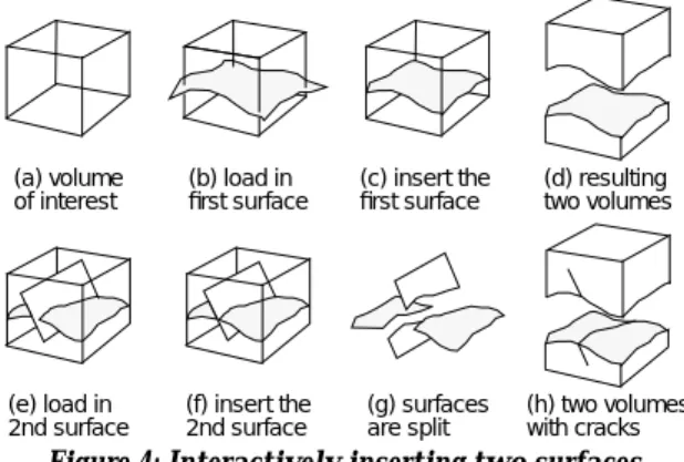
The geometric model is built incrementally by inserting surfaces into a volume of interest. The surface insertion involves Boolean operations. Surfaces intersect each other creating new 2-cells and new 3-cells which split the volume of interest into many subvolumes. Figure 4 illustrates an example. Figure 4-(a) shows the volume of interest (VOI). Figure 4-(b) brings in the first surface. We insert the first surface into the VOI. The Boolean operation trims the first surface by the boundary of the VOI (Figure (c)) and splits the VOI into two subvolumes (Figure (d)). The second surface is then loaded in (Figure 4-(e)) and inserted into the VOI. This action splits the first and second surfaces (Figure 4-(g)) and inserts cracks into the two subvolumes (Figure 4-(h)). A typical geoscience geometric model may be built from dozens or hundreds of surfaces. During model building it is important that a user can visualize and interactively edit the model.
3
SIGMA Surface Representation
The SIGMA surface representation [1] is novel as it extends traditional multiresolution surface techniques to geometric model building. In particular, data structures, typically used in computer graphics, are extended to support Boolean operations, and, as shall be shown in this paper, for interactive visualization and building of geometric models.
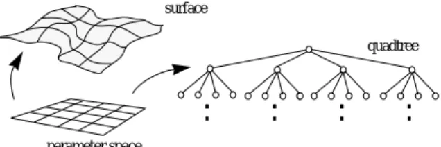
The SIGMA surface representation is a multiresolution hierarchy implemented as a quadtree [15]. The quadtree is built in the parameter space of structured grid data. Leaves of the quadtree contain a collection of triangles which are the triangulation of the grid cells the quadtree leaf node covered. In this way each triangle of the surface is assigned to a unique quadtree leaf node and a node of the quadtree inherits the triangles and vertices of its descendants. Figure 5 shows an example of a surface, its parameter space, and its quadtree.
Figure 2: Conventional data flow for adaptive visualization.
data
surface rep for geometry
modeling
geometric model for adaptive visualization multiresolution rep
graphics primitives construct
Boolean
decimate
update
construct
Figure 3: Data flow in SIGMA approach. data
SIGMA surface rep
geometric model
graphics primitives construct
Boolean update
decimate
multiresolution
Figure 4: Interactively inserting two surfaces. (a) volume
of interest
(b) load in first surface
(c) insert the first surface
(d) resulting two volumes
(e) load in 2nd surface
(f) insert the 2nd surface
(g) surfaces are split
(h) two volumes with cracks
The quadtree aids in model building as it supports triangle refinement. In particular, if a triangle is refined the refining triangles are assigned to the quadtree node of the original triangle. The quadtree also aids in computing maximal connected components as many of the quadtree nodes are connected.
Definition: A collection of nodes, C, of the tree T is a
node front if every leaf node of T has at most one
ancestor in C (a node is an ancestor of itself). A node front is a complete node front if every leaf node of T has exactly one ancestor in C.
Figure 6 shows an example of a complete node front. For a complete node front each triangle of the surface
belongs to a unique node in the node front, on the other hand, a vertex of the surface maybe shared by several nodes. Given a complete node front, the vertices that are shared by three or more nodes, or are on the boundary of the surface and shared by two or more nodes, are called critical vertices. Figure 7 shows how the critical vertices approximate the original surface and how they are represented in a quadtree with irregular boundaries. It can be shown, a constrained triangulation in parameter space of the critical vertices of a complete node front describes a decimated non-cracked view of the surface [1].
Terrain visualization has used the quadtree to achieve interactive rendering performance [17], [18]. However, these techniques have not been applied to visualizing a non-manifold geometric model. We use the quadtree to build and visualize a non-manifold geometric model.
4
Adaptive Visualization for Interactive
Geometric Modeling
As mentioned earlier, SIGMA is designed for interactive geometric modeling of large geoscience models. We apply adaptive visualization to each step of the modeling process. This section describes our technique and the supporting algorithms. First we introduce the concept of model coherence.
4.1
Model Coherence
A model is coherent if the geometry of the cells agrees at all dimensions [19]. With piecewise linear geometry, a coherent model means the 0-cell 0-simplices and 1-cell 1-simplices are faces of the 2-1-cell 2-simplices. A model is built by surface insertions (Section 2). Insertion includes two major steps, classification and making coherent. Classification is the topological operation that subdivides the point sets of operand geometries and determines the cells. Making coherent is the geometric operation that re-tessellates the mesh in the neighborhood of the intersection curve so 1-simplices of the curve are faces of 2-1-simplices of the mesh. Figure 8 shows an example of classification followed by making coherent. The classification results in two 2-cells A and B. We cannot geometrically separate A and B since triangles straddle both cells. After making coherent, each triangle belongs to a unique 2-cell. Making coherent is expensive, it is advantageous to visualize cells of an incoherent model as this permits viewing after classification.
4.2
The Role of Adaptive Visualization
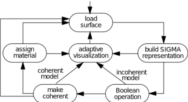
SIGMA enables adaptive visualization during the geometric modeling process. Both the model and individual surfaces can be visualized. To achieve performance, we decimate the surface and the model dynamically according to the viewing parameters. The decimation ensures no cracks are generated and preserves the intersection curves between surfaces in the model. For this purpose, critical vertices (Section 3) are used and the intersection curves are constraints during the model decimation. Figure 9 illustrates the role of adaptive visualization during interactive geometric modeling using SIGMA.
When a user loads a surface, SIGMA builds its surface representation. At this time, the surface is not part of the geometric model. Adaptive visualization algorithm applies to this individual surface. Inserting the surface into the volume of interest makes the
parameter space surface
quadtree
Figure 5: Parameter space and quadtree.
graph view
Black nodes are in the complete node front. geometric
view
Figure 6: Views of a complete node front.
0-cell vertex 1-cell vertex Internal vertex Original surface Decimated surface
Figure 7: Critical vertices at depths 1 and 2. Decimated surface
with level 1 nodes with level 2 nodes
Original cell Classified but not coherent Coherent A
B
surface a part of the model. The intersection curves between the surface and the volume of interest constrains the decimation. The geometric computation to insert a surface may be time consuming. The visualization algorithm can be applied before the computation completes, that is, visualizing an incoherent model.
When the user loads in the next surface, adaptive visualization can apply to the surface and the model independently. In other words, for adaptive visualization, the new surface is not subject to the constraints that surfaces in the model are. After insertion, the independent rendering behavior of this new surface is removed.
SIGMA can render physical material properties together with adaptive visualization of the geometry. Properties are rendered via per vertex coloring or via texture mapping.
4.3
Top Level Algorithm
Adaptive visualization refers to mechanisms that modify the visualization of objects according to given criteria. In this work, we dynamically decimate the geometric model according to camera position to achieve visualization performance.
A geometric model contains many surfaces (2-cells) and their intersections (1-cells). The decimation should be able to respect the macro-topology of the model. If each surface is decimated independently, there may be cracks between intersecting surfaces. To prevent cracking, the decimations are constrained with the same set of 1-cell edges for all the 2-cells intersecting at this 1-cell.
SIGMA adaptive visualization includes three major steps: vertex and edge selection, triangulation, and
rendering. The technique applies to individual
surfaces, coherent models, and incoherent models. An individual surface can be considered as a model with only one surface.
Selection: The module traverses each quadtree to select vertices and selects edges from each 1-cell in the model.
Triangulation: The module generates a triangle mesh for each surface (2-cell) from selected vertices and edges. The edges are constraints of triangulation. The vertex and edge selection and the triangulation together are referred to as decimation. Reference [1] describes a general decimation algorithm. This section presents a specific vertex selection algorithm for adaptive visualization. The decimation method in [1] is also extended for incoherent models.
Rendering: The module renders the triangle meshes. The physical material properties assigned to components of the geometric model can also be rendered.
Let M be a model, C be a set of criteria for vertex and edge selection, V be a set of selected vertices, and E be a set of selected edges. The following pseudocode sketches a top level algorithm for this technique.
while ((CameraMoved() == TRUE) and (|Projnew(M) - Projold(M)| > t)) { (V,E) := SelectVertexEdge(M, C); TM := Triangulate(M, V, E); UpdateGraphics(TM);}
where the CameraMoved function reports when camera has changed position; Proj function projects the model to the screen. When the change from the current projection to the previous projection is larger then a pre-specified threshold t, the model is re-decimated and graphics is updated. The Triangulate function may execute incremental and decremental algorithms instead of re-triangulating [20]. In addition to the camera movement and projection conditions, we also provide several options for users to control how often to update decimation during interactive visualization.
4.4
Vertex and Edge Selection
Vertex selection is performed for each quadtree in a model. The selection algorithm finds a node front of a quadtree via traversing the tree. Critical vertices of the node front form the subset of vertices to be rendered. Two major operations involved during the traversal are: view frustum culling and projection. View frustum culling determines those parts of the surface that are outside of the view frustum and need not be rendered. Projection determines the decimation resolutions of the surface.
Each quadtree node has a bounding object that bounds the triangles of the node. The algorithm traverses the quadtree from its root node. If the bounding object of a node is outside the view frustum, the node need not be visualized; and traversal continues to the next node. Otherwise, the bounding object of the node is projected to the screen. If the projected area is smaller than a pre-specified minimum resolution, the node is in the node front. Otherwise, the traversal needs to resolve the children of the node.
Figure 9: The role of adaptive visualization. adaptive
visualization representationbuild SIGMA surface
load
Boolean make
coherent assign
material
incoherent model coherent
model
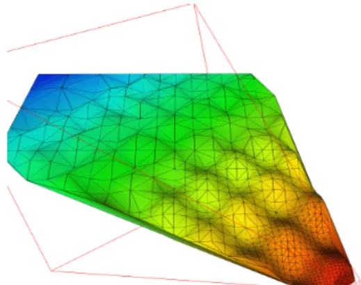
Due to perspective viewing, critical vertices from the node front results in a mesh with varying resolution. The portion of the surface closest to the camera has finer resolution. Further from the camera, the surface has coarser resolution. See Figure 13.
For an incoherent model, more than one 2-cell might share the same quadtree. In this case, each quadtree is still traversed once for vertex selection. To simplify edge selection and triangulation, 1-cells in an incoherent model are made coherent. This is not expensive and needs to be done only once.
There are the following cases for edge selection: 1. Visualizing an individual surface.
1.1 The surface has a convex boundary in its parameter space and has no holes.
1.2 The surface has a non-convex boundary in its parameter space or has holes. The bound-ary, including the holes, is represented by 1-cells.
2. Visualizing a geometric model that contains 1-cells and 2-1-cells. Some of the 1-1-cells represent intersec-tions between 2-cells.
For case 1.1, edge selection is not required. For other cases, edge selection is done by decimating 1-cells. The vertex and edge selection algorithm can be written in the following pseudocode,
SelectVertexEdge(M, C): for each quadtree T in M
V += Traverse(T, C);
E := DecimateOneCells(M, C); return (V,E);
where the Traverse function traverses quadtree T as described earlier. The camera parameters and pre-specified screen resolution are encoded in parameter
C. The result of Traverse is a set of selected vertices.
The DecimateOneCells function finds all the 1-cells in model M and decimates them to obtain edges.
4.5
Triangulation
We use Delaunay triangulation [21], [22] to triangulate selected vertices in the parameter space of a surface. When edges are present, constrained Delaunay triangulation is applied to the vertices with edges as constraints. The resulting triangle mesh is mapped to the image space to approximate the original surface. During interaction, the camera moves and many vertices selected are repeated from one position to the next. Incremental and decremental Delaunay triangulation [20] can be used to update the mesh. The triangulation applies progressively more constraints to the three cases listed in the previous section. For case 1.1 where a surface has a convex boundary and no holes, Delaunay triangulation applies to the selected vertices. For case 1.2 where a
surface has non-convex boundary or has holes, constrained Delaunay triangulation is used.
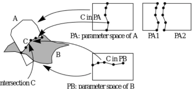
For case 2 where a model is visualized, to preserve intersection curves, constrained Delaunay triangulation is used for each 2-cell in the model. Given a 2-cell, edges from all its 1-cells are constraints to the triangulation. To prevent cracking, for each 1-cell, the same set of edges from the 1-cell constrains all the 2-cells intersecting at this 1-cell. Figure 10 shows an example. Surfaces A and B intersect. The
intersection curve C is a 1-cell. Surface A is split into two 2-cells, A1 and A2. Surface B is still one 2-cell, but has a crack resulting from the intersection. The 1-cell C is shared by three 2-cells, A1, A2, and B. Figure 10 shows the parameter spaces of A, B, A1, and A2. During the edge selection (Section 4.4), C is decimated. In this example, the decimated version of C has four edges. During triangulation, for each 2-cell, B, A1, and A2, we find edges of C in the 2-cell’s parameter space, respectively (Figure 10). The edges are part of the triangulation constraints in 2-cells’ parameter spaces.
The triangulation algorithm is sketched in the following pseudocode,
Triangulate(M, V, E): for each 2-cell S in M {
VP:= V.getVerticesInParamSpace(S); B := S.getBoundaryCells();
EB := E.getEdges(B);
EP := EB.getEdgesInParamSpace(S); TM+= ConstrainedDelaunay(VP, EP);} return (TM);
where getEdgesInParamSpace function maps the boundary edges EB of S to the parameter space of S.
The ConstrainedDelaunay function executes in
parameter space of S. This algorithm is straightforward for a coherent model since each 2-cell has its own quadtree and a set of selected vertices from the quadtree. The algorithm also works for an incoherent model as explained below.
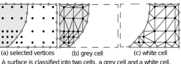
In an incoherent model, a quadtree may be shared by multiple 2-cells. Therefore, given a 2-cell, some of the selected vertices from the quadtree may not be part of the 2-cell. Figure 11 shows an example. A surface is classified into grey cell and white cell, but has not
A
B
PA: parameter space of A
PB: parameter space of B intersection C
C
C in PA
C in PB
PA1 PA2
been made coherent. Both the grey cell and the white cell share the same quadtree of the original surface. Figure 11-(a) shows selected vertices from the quadtree and selected edges from 1-cells. Vertices on the white cell are not part of the grey cell, and vice versa. Constrained Delaunay triangulation is applied to each 2-cell separately. Figure 11-(b) and (c) shows the constrained Delaunay triangulations for the grey cell and white cell, respectively. Since each 2-cell has a closed boundary of 1-cells, the vertices outside of the boundary are removed during triangulation. With this approach, one traversal for vertex selection is done for each quadtree. The triangulation runs as many times as the number of 2-cells sharing this quadtree.
4.6
Performance versus Quality
SIGMA is deployed on a wide-range of visualization hardware. It is important a user is given a broad range of rendering options to maintain interactive performance. As has been described in previous sections, SIGMA can reduce triangle counts by using decimation and culling. However, SIGMA permits another group of trade-offs which are based around the visualization of the geometric model. In particular, it is possible to trade-off topological quality for performance, see Figure 12.
For optimum quality, the model is rendered at full resolution. To improve rendering performance the model can be decimated. However, decimating the model may introduce topological artifacts such as cracking and bubbling. Preventing these topological artifacts, especially bubbling, is costly and a user may decide such topological quality is unnecessary. The surfaces can be decimated even further until they have no interior points and are only defined by their boundaries. One can even drop the surfaces altogether
and just draw the 1-cell wireframe of the model. Finally, a crude approximation of the model can be given by rendering bounding boxes of the surfaces. These trade-offs can be chosen by users at the application level.
5
Application
To support interactive geometric modeling in geoscience, we developed the Common Model Builder [23], [16], which is an application-neutral framework. SIGMA is embedded in the Common Model Builder.
Figure 13 shows the adaptive visualization of a synthetic surface. The z value of the surface is defined by sine functions of x and y values. Figure 13-(a) is a scene viewed by a user. The surface is adaptively decimated and is rendered with a space varying property. Figure 13-(b) shows a bird’s eye view of the surface, where the red outlined polyhedron is the view frustum. The camera is at the lower right corner. We can see triangles are of smaller size near the camera, and their sizes increase away from the camera.
Figure 14 show snapshots from a geoscience geometric modeling process using SIGMA. Surfaces in these figures are rendered with adaptive visualization technique. There are two model display modes: surface mode and volume mode.
In Figure 14-(a), an unconformity surface is inserted into the volume of interest (VOI). This operation splits VOI into two volumes (Figure 14-(b)). Figure 14-(c) is an explored view of the two volumes. The second surface has an older geological age. To ensure the validity of a geological model, we insert the second surface to the lower volume Figure 14-(d), which is split into two volumes Figure 14-(e). In Figure 14-(f), we insert four more surfaces into the model. Figure 14-(g) shows the volume view of the model. The top volume has been assigned a physical material property, which is mapped into a colormap in order to render. In Figure 14-(h), we take off the top volume to show some details inside the model. Figure 14-(i) has three fault surfaces added to the mode.
6
Conclusion
This paper presents an adaptive visualization solution for interactively building large high resolution geometric models. Distinct from existing approaches, adaptive visualization applies during model construction. The same multiresolution surface representation is used for visualization and Boolean computations. The representation is incrementally updated, rather than reconstructed, when the model changes. We have developed techniques that adaptively decimate models (coherent and incoherent), according to camera position. The decimation algorithm preserves intersection curves between surfaces in the model. The technology is Figure 11: Triangulation of incoherent 2-cells.
(a) selected vertices (b) grey cell (c) white cell A surface is classified into two cells, a grey cell and a white cell.
full
decimate not preserving
intersection curves (b)
convex hulls
1-cell
bounding boxes
performance quality
Figure 12: SIGMA provides a range of selections for performance and quality.
(a) + lower resolution or LOD
(b) + lower resolution or LOD decimate
preserving intersection curves (a)
boundary defined
surfaces wireframe resolution
perfect
topology macro
embedded into a 3D geoscience geometric modeling application framework. Disciplines other than geoscience face similar problems when building large geometric models; SIGMA technology may be applicable. Many optimizations remain to be developed to improve SIGMA, which is the main focus of our future work.
6.1
Acknowledgements
We would like to thank Eric Schoen, Christoph Ramshorn and Steven Assa for their help in this work, and Doug Palkowsky for providing datasets.
7
References
[1] R. Hammersley, H.Q. Lu, and S. Assa. Geometric Modeling with a Multiresolution Representation.
In Proceedings of the Eleventh Canadian Conference on Computational Geometry, Vancouver, Canada, August 15-18, 1999.
[2] M. Eck, T. DeRose, T. Duchamp, H. Hoppe, M. Lounsbery, and W. Stuetzle. Multiresolution analysis of arbitrary meshes. In Proceedings of
SIGGRAPH’95, pages 173-182, ACM, New York, 1995.
[3] M. Garland, and P. Heckbert. Surface
Simplification Using Quadric Error Metrics. In
Proceedings of SIGGRAPH’97, pp 209-216.
[4] H. Hoppe. Progressive Meshes. In Proceedings of
SIGGRAPH’96, pp 99-108, 1996.
[5] W. Schroeder, J. Zarge, and W. Lorensen. Decimation of Triangle Meshes. In Proceedings of
SIGGRAPH’92, pages 65-70.
[6] A. Lee, H. Moreton and H. Hoppe. Displaced Subdivision Surfaces, In Proceedings of
SIGGRAPH 2000, pages 85-94, 2000.
[7] I. Guskov, K. Vidimce, W. Sweldens, P. Schroder. Normal Meshes, In Proceedings SIGGRAPH 2000, pages 95-102, 2000.
[8] L. Kobbelt. -Subdivision, In Proceedings of
SIGGRAPH 2000, pages 103-112, 2000.
[9] E. Catmull and J. Clark. Recursively Generated B-Spline Surfaces on Arbitrary Topological Meshes. Computer-Aided Design, vol. 10, pages 350-355, 1978.
[10] W. Xu and D. Fussell. Multiresolution of Arbitrary Triangular Meshes. Presented at
SIGGRAPH’98 Sketches, 1998.
[11] D. Zorin, P. Schroder, and W. Sweldens. Interpolating Subdivision for Meshes with Arbitrary Topology. In Proceedings of
SIGGRAPH’96, pages 189-192.
[12] L. Kobbelt, S. Campagna, J. Vorsatz, and H. Seidel. Interactive Multiresolution Modeling on Arbitrary Meshes. In Proceedings of
SIGGRAPH’98, pp 105-114, 1998.
[13] M. Lounsbery, T.D. DeRose, and J. Warren.
Multiresolution Analysis for Surfaces of Arbitrary
Topological Type. ACM Transactions on Graphics,
16(1), pages 34-73, 1997.
[14] E. Stollnitz, T. DeRose, and D. Salesin. Wavelets for Computer Graphics - Theory and
Applications. Morgan Kaufmann Publishers, Inc., 1996.
[15] H. Samet. The Design and Analysis of Spatial Data Structures. Addison-Wesley Series in Computer Science 1990. ISBN 0-201-50255-0. [16] S. Assa, G. Celniker, and C. Ramshorn,
Feature-Based Geometric Modeling for Geoscience, GOCAD
ENSG Conference, 3D Modeling of Natural Objects: A Challenge for the 2000’s, June 1998. [17] M. Gross, O. Staadt, and R. Gatti. Efficient
Triangular Surface Approximations Using Wavelets and Quadtree Data Structures. IEEE Trans.
Visualization and Computer Graphics, 2(2), pages 130-143, 1996.
[18] R. Pajarola. Large Scale Terrain Visualization using the Restricted Quadtree Triangulation. In
Proceedings of Visualization’98, pages 19-26.
[19] SHAPES Reference Manual, Release 2.1.2, 1995. XOX Corporation.
[20] R. Hammersley and H.Q. Lu. Decremental Delaunay Triangulation. Presented at SIGGRAPH
‘99 Technical Sketch.
[21] S. Fortune, Voronoi Diagrams and Delaunay
Triangulations, In F.K. Hwang and D.-Z. Du,
editors, Computing in Euclidean Geometry, 2nd edition, pages 225-265, World Scientific, Singapore, 1995.
[22] J. R. Shewchuk. Triangle: Engineering a 2D Quality Mesh Generator and Delaunay Triangulator. In Proceedings of First ACM
Workshop on Applied Computational Geometry, pages 124-133, May 1996.
[23] H.Q. Lu, E. Schoen, J. Salim, Y. Cudennec, and C. Ramshorn. Common Model Builder -- A Toolkit for Multidisciplinary Geoscience Modeling Applications. In Proceedings of GOCAD ENSG
Conference, 3D Modeling of Natural objects: A Challenge for the 2000’s, June 1998.
Figure 13: Adaptive visualization of a surface.
(a) The surface seen by a user. (b) A bird’s eye view of the surface.
Figure 14: Snapshots from a modeling sequence (images from left to right, top to bottom).
(a) (b) (c)
(d) (e) (f)