The Astronomical Journal, 137:3761–3777, 2009 April doi:10.1088/0004-6256/137/4/3761
C
2009. The American Astronomical Society. All rights reserved. Printed in the U.S.A.
ULTRAVIOLET QUASI-STELLAR OBJECTS
Luciana Bianchi1, John B. Hutchings2, Boryana Efremova3, James E. Herald3, Alessandro Bressan4,5,
and Cristopher Martin6
1Department of Physics and Astronomy, Johns Hopkins University, 3400 North Charles Street, Baltimore, MD 21218, USA; [email protected] 2The National Research Council of Herzberg Institute of Astrophysics, Canada
3Center for Astrophysical Sciences, Johns Hopkins University, Baltimore, MD, USA 4INAF–Astronomical Observatory of Padova, Padova, Italy
5INAOE, Tonantzintla (Puebla), Mexico 6California Institute of Technology, Pasadena, CA, USA
Received 2008 May 20; accepted 2008 December 27; published 2009 March 4
ABSTRACT
We present a sample of spectroscopically confirmed quasi-stellar objects (QSOs) with FUV–NUV color (as measured by Galaxy Evolution Explorer (GALEX) photometry, FUV band: 1344–1786 Å, NUV band: 1771– 2831 Å) bluer than canonical QSO templates and than the majority of known QSOs. We analyze their FUV to NIR colors, luminosities, and optical spectra. The sample includes a group of 150 objects at low redshift (z < 0.5), and a group of 21 objects with redshift 1.7 < z < 2.6. For the low-redshift objects, the “blue” FUV–NUV color may be caused by enhanced Lyα emission, since Lyα transits the GALEX FUV band from z = 0.1 to
z = 0.47. Synthetic QSO templates constructed with Lyαup to three times stronger than in standard templates match the observed UV colors of our low-redshift sample. Optical photometric and spectroscopic properties of these QSOs are not atypical. The Hαemission increases, and the optical spectra become bluer, with increasing absolute UV luminosity. The lack of selected objects at intermediate redshift is consistent with the fact that for
z=0.48–1.63, Lyαis included in theGALEXNUV band, making the observed FUV–NUV redder than the limit of our sample selection. The UV-blue QSOs at redshift ∼2, where theGALEX bands sample rest-frame≈450– 590 Å (FUV) and ≈590–940 Å (NUV), are fainter than the average of UV-normal QSOs at similar redshift in NUV, while they have comparable luminosities in other bands. Therefore, we speculate that their observed FUV– NUV color may be explained by a combination of steep flux rise toward short wavelengths and dust absorption below the Lyman limit, such as from small grains or crystalline carbon (nanodiamonds). The ratio of Lyα to C iv could be measured in 10 objects; it is higher (30% on average) than for UV-normal QSOs, and close
to the value expected for shock or collisional ionization. However, optical spectra are taken at different times than the UV photometry, which may bias the comparison if lines are variable. These QSO groups are uniquely set apart by the GALEX photometry within larger samples, given that their optical properties are not unusual.
Key words: quasars: absorption lines – quasars: emission lines – quasars: general – ultraviolet: galaxies
Online-only material:color figures, machine-readable and VO tables
1. INTRODUCTION
In all quasi-stellar object (QSO) samples, there is con-cern that selection effects are present and significant, partic-ularly in whether whole classes of objects are not included, or even known. This study aims at characterizing a popu-lation of objects with rising fluxes at UV-observed wave-lengths. Following our work of classification of UV sources from the GALEX7 sky surveys (Bianchi 2008; Bianchi et al.
2005,2006,2007,2008; Hutchings & Bianchi2008 and ref-erences therein), we have suspected the existence of a sub-stantial number of extragalactic objects with FUV–NUV color much bluer (more negative) than canonical QSO templates and than the majority of QSOs in known samples. Such ob-jects are rather “normal” at optical wavelengths (spectroscop-ically and photometr(spectroscop-ically) but they stand out in the ob-served UV range, having FUV–NUV colors similar to those
7 TheGalaxy Evolution Explorer(GALEX; Martin et al.2005), is a NASA Small Explorer performing imaging surveys of the sky in two UV bands simultaneously: FUV (1344–1786 Å,λeff=1538.6 Å) and NUV (1771– 2831 Å,λeff=2315.7 Å) with different coverage and depth. See Bianchi (2008) for a summary of the UV sources classification and statistics in the main surveys, and Morrissey et al. (2007) for instrument description and performance.
of hot white dwarfs (WDs). Photometrically, these objects have UV-to-optical colors similar to a stellar binary containing a hot WD and a cooler companion. That a significant number of “FUV–NUV” blue extragalactic objects existed was first sus-pected by Bianchi et al. (2007), based on density counts of photometrically selected WD candidates. In fact, the number of objects per square degree whose spectral energy distribu-tion (SED; FUV to NIR) is consistent with a single hot WD increases with magnitude down to mUV ∼ 21 (AB) and then declines, consistent with Milky Way (MW) models. However, the density of objects with similarly blue UV color but redder optical colors, that we would expect to be hot WDs with a cool companion, increases considerably at fainter magnitudes, sug-gesting that a significant number of faint extragalactic objects may be included in the color–colorlocusof these stellar bina-ries (Bianchi et al.2007; Bianchi2008). In this work, we focus on these QSOs, which display very blue observed FUV–NUV colors, and investigate whether their properties are unlike those of known objects.
2. SAMPLE AND DATA
The sample was extracted from the catalog of matched UV/
optical sources of Bianchi (2008), obtained by matching the
UV sources in the GALEX third data release (GR3),8 to the
Sloan Digital Sky Survey (SDSS) sixth data release (DR6).
GALEXprovides sky surveys with different sky area coverage
and depth: we restricted this work to the “Medium Imaging Survey” (MIS) data, which reaches a typical AB mag of≈22.7 in both FUV and NUV. The overlap area betweenGALEX-GR3 MIS data and SDSS-DR6 is 573 deg2 (Bianchi 2008), taking
into account that only the central 1◦diameter part of theGALEX
fields was used in our master catalog, to assure homogeneous photometry quality and exclude defects in the outer parts of the circular field. For each matched source,GALEXprovides FUV (1344–1786 Å, λeff = 1538.6 Å) and NUV (1771–2831 Å,
λeff =2315.7 Å) photometry, and the SDSS providesu, g, r, i, z
photometry. More details on the matchings procedure and the catalog are given by Bianchi (2008) and L. Bianchi et al. (2009, in preparation).
In order to characterize the suspected “FUV–NUV blue” QSOs, we extracted from the matched UV/optical source catalog of Bianchi (2008) the spectroscopically confirmed QSOs with FUV–NUV < 0.1 (AB mag): this FUV–NUV limit is “bluer” (more negative) than the synthetic FUV–NUV color from the two QSO canonical templates used by Bianchi et al. (2007), which represent average QSO properties, at any redshift. The colors of the canonical templates are shown in Figures1
and2(cyan diamonds) as a function of redshift. We will refer to this sample as “UV-blue” QSOs for brevity throughout the paper. It is restricted to sources with photometric errors smaller than 0.3 mag in both FUV and NUV, and color FUV–NUV<
0.1, for which SDSS spectroscopy exists and gives a “QSO” classification. The requirement of available SDSS spectroscopy effectively limits the sample to brighter magnitudes, but it provides a classification and useful information, which will help interpreting larger samples of photometric candidates. Such relatively bright objects will also be accessible to the spectroscopic capabilities of the refurbished Hubble Space
Telescope (HST), and to other follow-up observations. Note
that the SDSS spectroscopic class “QSO” (class 4) probably also includes Seyfert galaxies. We will use here the generic term “QSO” to reflect our selection criterion from the SDSS spectroscopic database. It is important to note that spectroscopic targets in the SDSS were selected with criteria unrelated to our present objective and therefore our UV-blue spectroscopically confirmed QSOs may be a biased subsample among the UV-blue QSO photometric candidates.
These selection criteria produced an initial sample of 174 objects. One additional object was excluded because itsu-band measurement is saturated. The photometric properties of the sample QSOs are presented in Section3, and their optical spectra and overall properties are analyzed in Section4. The selected objects are shown in two color–color diagrams, Figures 1
and 2, where they can be compared with other classes of objects, in particular hot stars, typical QSOs, and galaxies. Our analysis of the spectra (Section4) generally confirms the redshift measurement from the pipeline. However, we found that one object (GALEX J172101.08+532433.7, R.A. =260.2544916, decl.=53.4093516, SDSS match id=587725490527731868) was misclassified by the SDSS spectroscopic pipeline as a QSO with redshiftz=2.7: its spectrum is that of a hot star. It is shown in some figures because it is interesting to note its position in the color–color diagrams (Figures1and2): theGALEXphotometry clearly place this object on the stellar sequence and not as a
8 GR3 is available from the MAST archive athttp://galex.stsci.edu.
Figure 1.Color–color diagram showing the catalog of GR3-MIS UV sources of Bianchi (2008), with blue dots for pointlike sources and black dots for extended sources (essentially galaxies). Our UV-blue QSOs are shown with teal dots (circled for extended sources, and marked with an X when the FUV–NUV error is>0.15). Synthetic colors for QSO templates are shown with diamonds (cyan: standard templates, dark blue: templates with three times enhanced Lyα
emission; dark green: templates withFλ ∼ λ−0.6 andFλ ∼λ−1.2 in EUV. The redshift values marked by the diamonds arez=0 (largest cyan diamonds, near the center), 0.2, 0.4, 0.6, 1.0, 1.2, 1.4, 1.6, 1.8, 2.0 (labeled), 2.2, 2.4, 2.6 (labeled), 3.0. Stellar sequences are shown (red, yellow, and purple triangles for logg = 3,5, and 9), withTeff values marked. A reddening arrow for
E(B−V)=0.3 is shown on a WD (Teff=30 kK) model point. The yellow star is the stellar object misclassified by the SDSS pipeline as a QSO. The majority of UV-normal QSO follows the template tracks, below and to the left of the stellar sequence.
QSO candidate. Coordinates, photometry, and other relevant information are given in Table1, and sample images are shown in Figure3.
The SDSS optical spectra (range∼3800–9200 Å, resolution
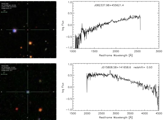
∼1800) provide the initial classification as QSOs and a measure of redshift for the objects. Our sample includes a group of 151 objects at low redshift (0.041 < z < 0.436), and 21 objects with redshift between 1.7 and 2.6, all pointlike. Only one object has intermediate redshift (z=0.93) and its identification as a QSO is dubious. It has fairly large photometric errors: FUV= 21.49±0.12, NUV=21.43±0.10, but the typical QSO FUV– NUV color at this redshift is much redder (by >1 mag, see Figure1); therefore, if it is a QSO it would be quite anomalous. At this redshift, theGALEXbands sample rest wavelengths of
∼1300 Å (NUV) and∼800 Å(FUV), and a very blue FUV– NUV color would not be expected. The image and spectrum of this object are shown in Figure4(bottom). The spectrum shows one emission line that is identified as Mg ii for the alleged
redshift and possibly a few absorptions including one at the red end that could be Hγ. The observed wavelengths of the lines are not obvious for identification, assuming other values of redshift the observed line(s) might be [Ciii]λ1909 or [Oii]λ3727, but
then other lines such as [Civ]λ1550 or [Oiii]λ5007 should be
present and are not. So, eitherz=0.93 is right or perhaps the emission is some artifact in the spectrum. Therefore, we consider this object doubtful and do not include it in our analysis. The lack of objects between redshift 0.5 and 1.7 is consistent with our selection of very blue FUV–NUV color, because Lyαis in the NUV band betweenz=0.48 andz=1.63, causing brighter
No. 4, 2009 EUV QSOs 3763
Figure 2.Color–color diagram including theg−icolor. Symbols as in previous figure. In this plot, the NUV–gcolor separates the high- and low-redshift QSOs (redshift values marked in cyan along the template,z=0 is the large diamond at the top of the sequence. The cluster of pointlike sources close to the low-z QSO template colors are normal QSOs. The extended sources among our UV-blue QSOs haveg−iredder than QSOs templates, and in theg−icolor range of galaxies, reflecting the contribution from the underlying galaxy, but they are bluer than the galaxies in NUV–g. This diagram further separates the single hot stars from the UV-blue QSOs (note again the location of the spectroscopically misclassified object, plotted as a yellow star).
flux in NUV and consequently much redder FUV–NUV color, as can be seen in Figure1.
We also caution that while the GALEX FUV and NUV images are taken simultaneously, the SDSS imaging was taken at a different time from the GALEX observations, therefore any significant variability may affect the combined UV and optical colors, such as NUV–r. For this reason, we based our initial sample selection on the FUV–NUV color only. Some of our targets have repeated observations withGALEX, but most repeated measurements are from the All-sky Imaging Survey (AIS), which has about 10 times shorter exposures than MIS (used in this work) and therefore large photometric uncertainties. In a few cases, repeated measurements are discrepant by>2σ
in the combined photometric errors: however, most of the discrepant measurements have artifact flags set. We compile for completeness all repeated measurements with exposures longer than 400 s and formally discrepant by>2σ in Table2, where we also provide comments that help assess reliability, based on the flags from the pipeline photometry, and our visual inspection of the images. We only excluded measurements on the very edge of the GALEX field (flag “rim”), however we did not apply error cuts nor area cut, for the purpose of an exhaustive comparison, while our analysis sample is restricted to measurements in the central 0.◦5 radius of the field for accurate photometry (Section 2). In a few cases, the discrepancies in the repeated measurements cannot be ascribed to artifacts, and these objects may deserve dedicated follow-up photometry. In some cases the variation affects the FUV–NUV color, and in particular some repeated measurements have redder FUV–NUV than our initially selected data set. All discrepant repeated
measurements with MIS exposures (two high-redshift objects and 10 low-redshift objects) have FUV–NUV >0.1. If we also consider AIS data (exposure times ∼100 s), we find 55 additional repeated measurements discrepant by >2σ, of which 36 give FUV–NUV redder than our selected data set (MIS measurements), and other 19 bluer. Fast variability is not unknown in QSOs, and in particular line strength may vary on short timescales, while it would be less plausible for dust effects to change rapidly. We stress that a variability assessment however would require custom photometry, and while the standard pipeline photometry is good for statistical analysis, such as the scope of this work, we should refrain from overinterpreting individual measurements and individual variations. Other 72 AIS and seven MIS repeated measurements agree within 2σ with our selected measurements given in Table1. One object in the initial sample, although part of the MIS survey, has a 40 s exposure in FUV and 1518 s in NUV: although its FUV error (0.23) meets our selection limits, a longer MIS exposure of 853 s in both FUV and NUV and smaller errors gives FUV–NUV=0.17, so it is eliminated from our analysis sample.
A larger sample of about 30,000 QSO candidates with “nor-mal” FUV–NUV colors (i.e., similar to the standard tem-plate), extracted from the matched UV/optical source catalog of Bianchi (2008) will be presented elsewhere. We will refer to this sample as “UV-normal” in the discussion of the UV-blue sample for comparison purposes.
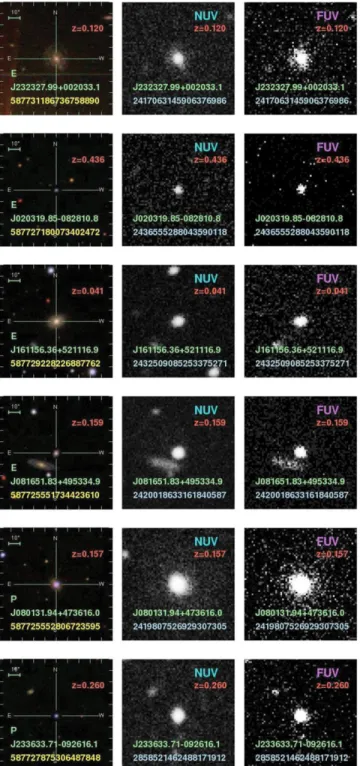
3. GENERAL PHOTOMETRIC PROPERTIES Of the 174 sample objects, 64 sources are classified as pointlike (at the resolution of the SDSS imaging,∼ 1.4) and 110 as extended (all at low redshift), by the SDSS pipeline. We will keep the pipeline classification because it is derived from an objective procedure, although the result depends on the contrast between central source and underlying galaxy. GALEX and SDSS imaging for a subsample of objects, presented in Figure3, shows that the definition of “pointlike” (P) or “extended” (E) is not clear-cut.
The sample selection, as described in Section 1, was re-stricted to MIS sources with photometric errors less than 0.3 mag in FUV and NUV. Of the 64 pointlike sources, 42/33 have errors less than 0.1 mag/0.05 mag, and only four have errors between 0.2 and 0.3 mag, in FUV. As for the NUV mea-surements, 36/45 pointlike sources have errors<0.05/0.1 mag, and 10 have errors larger than 0.2 mag. In therband, all but two objects have errors smaller than 0.05 mag (one object has an error of 0.14 mag, and one of 0.08 mag). Of the 110 ex-tended objects, 108 haver-band error<0.04 mag, 97/94 have NUV/FUV error <0.1 mag. Sources with large photometric errors are identified in the figures. Most objects with larger errors are in thez ∼ 2 group. At this redshift, our color cut of FUV–NUV<0.1 is more than half a magnitude bluer than the average value for UV-normal QSOs (e.g., Figure1), there-fore these objects may be truly extreme with respect to av-erage samples in spite of their large photometric errors. We point out that the object GALEX J113223.4+641958 (SDSS J113223.42+641958.4) has au-band magnitude of 28.7±0.46 (petromag), while the magnitude listed on the explorer page for this object is u = 25.07±3.05. It has no artifact flags, the pipeline records only a warning: “no petrosian radius could be determined. Petrosian magnitude still usable; the object is blended with an extended object.” The surrounding galaxy can be seen in the SDSS imaging with a radius of about 5. We regard
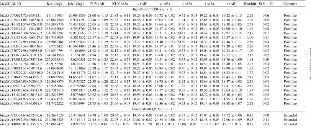
BIANCHI ET AL. V ol. 137 Table 1
The UV-Blue QSO Sample
GALEXIAU ID R.A. (deg) Decl. (deg) FUV (AB) NUV (AB) u(AB) g(AB) r(AB) i(AB) z(AB) Redshift E(B−V) Comment
High-Redshift QSOs (z >1) GALEXJ075627.72+205415.1 119.1154984 20.9041836 21.00±0.15 21.82±0.14 20.23±0.09 19.72± 0.02 19.52±0.03 19.22±0.04 19.22± 0.15 2.21 0.06 Pointlike GALEXJ025221.08−085516.0 43.0878540 −8.9211193 20.88±0.09 21.67±0.11 18.56±0.03 18.03± 0.01 17.94±0.01 17.85±0.02 17.50± 0.04 2.29 0.05 Pointlike GALEXJ161821.57+492603.0 244.5898736 49.4341532 22.05±0.18 22.74±0.23 19.23±0.04 18.64± 0.01 18.66±0.01 18.63±0.02 18.38± 0.05 2.28 0.02 Pointlike GALEXJ222323.21−084740.5 335.8467089 −8.7945764 22.35±0.14 23.01±0.25 19.52±0.05 19.47± 0.02 19.38±0.02 19.14±0.03 19.00± 0.10 1.99 0.05 Pointlike GALEXJ145645.30+595436.2 224.1887297 59.9100553 22.57±0.19 23.14±0.29 20.52±0.08 20.31± 0.03 20.41±0.04 20.44±0.07 19.97± 0.15 2.17 0.01 Pointlike GALEXJ211858.56−063027.3 319.7439988 −6.5075842 22.17±0.17 22.58±0.19 19.97±0.06 19.75± 0.02 19.62±0.02 19.48±0.04 19.27± 0.11 2.00 0.11 Pointlike GALEXJ082337.98+455621.4 125.9082468 45.9392840 22.41±0.19 22.67±0.29 22.22±0.80 21.40± 0.23 20.86±0.14 20.33±0.09 19.46± 0.11 2.59 0.04 Pointlike GALEXJ003505.58−103536.4 8.7732425 −10.5934493 22.46±0.23 22.68±0.25 19.35±0.04 18.57± 0.01 18.62±0.01 18.49±0.01 18.20± 0.05 2.26 0.03 Pointlike GALEXJ230724.98+000958.0 346.8540794 0.1661096 21.93±0.15 22.12±0.10 19.40±0.06 19.41± 0.02 19.33±0.03 19.04±0.03 19.23± 0.17 1.90 0.04 Pointlike GALEXJ113638.68+011031.5 174.1611550 1.1754105 21.94±0.18 22.13±0.20 19.83±0.05 19.68± 0.02 19.60±0.03 19.47±0.04 19.17± 0.11 2.13 0.02 Pointlike GALEXJ155013.52+033744.6 237.5563540 3.6290531 22.74±0.25 22.86±0.27 19.54±0.05 19.51± 0.02 19.33±0.02 18.93±0.03 18.76± 0.09 1.91 0.10 Pointlike GALEXJ233139.76+010428.7 352.9156781 1.0746313 20.56±0.07 20.67±0.07 18.93±0.03 18.54± 0.01 18.45±0.01 18.53±0.01 18.40± 0.05 2.25 0.04 Pointlike GALEXJ090814.51+550701.6 137.0604696 55.1171069 22.98±0.17 23.03±0.22 20.21±0.06 19.84± 0.02 19.46±0.02 19.07±0.02 18.90± 0.08 1.93 0.02 Pointlike GALEXJ015229.22−083640.0 28.1217418 −8.6111176 22.43±0.19 22.47±0.19 20.27±0.10 19.84± 0.03 19.27±0.03 18.84±0.03 18.83± 0.11 1.72 0.02 Pointlike GALEXJ020419.29+143929.2 31.0803956 14.6581219 21.07±0.11 21.11±0.09 19.11±0.03 18.85± 0.01 18.80±0.01 18.61±0.02 18.43± 0.06 2.17 0.05 Pointlike GALEXJ082616.05+502049.5 126.5668879 50.3470827 22.58±0.20 22.61±0.27 19.19±0.04 18.75± 0.01 18.62±0.01 18.60±0.02 18.37± 0.05 2.19 0.04 Pointlike GALEXJ005408.42−094637.1 13.5350664 −9.7769584 22.64±0.28 22.68±0.24 18.45±0.02 18.06± 0.01 17.82±0.01 17.61±0.01 17.41± 0.03 2.13 0.04 Pointlike GALEXJ145055.62+015419.0 222.7317516 1.9052814 21.48±0.12 21.45±0.12 19.86±0.05 19.77± 0.02 19.75±0.03 19.56±0.04 19.63± 0.18 1.87 0.04 Pointlike GALEXJ141807.07+050431.3 214.5294395 5.0753685 20.92±0.09 20.87±0.06 19.93± 0.06 19.56± 0.02 19.10±0.02 18.72±0.02 18.46± 0.05 1.89 0.03 Pointlike GALEXJ085344.92+565337.9 133.4371727 56.8938634 21.71±0.13 21.63±0.11 20.42±0.14 20.45± 0.05 20.40±0.08 20.12±0.10 21.35± 1.50 1.86 0.05 Pointlike GALEXJ084658.13+465011.4 131.7422222 46.8364994 21.75±0.08 21.66±0.08 19.47±0.04 19.36± 0.02 19.24±0.02 19.14±0.03 18.88± 0.07 2.12 0.02 Pointlike Low-Redshift QSOs (z <1) GALEXJ075304.64+252436.6 118.2693129 25.4101641 19.78±0.08 20.67±0.06 19.36±0.07 18.84± 0.02 18.33±0.02 17.94±0.02 17.72± 0.06 0.15 0.09 Extended GALEXJ154912.35+030641.8 237.3014425 3.1116111 22.45±0.28 22.95±0.28 21.62±0.57 20.34± 0.06 19.01±0.03 18.48±0.03 17.96± 0.09 0.25 0.13 Extended GALEXJ140816.07+015528.5 212.0669475 1.9245728 22.26±0.18 22.73±0.29 20.50±0.28 19.11±0.03 18.06±0.02 17.61±0.02 17.23±0.05 0.17 0.03 Extended
No. 4, 2009 EUV QSOs 3765
Figure 3.Sample imaging of our UV-blue QSOs. Each row shows one object. Columns left to right—first: color-composite SDSS image (resolution≈1.4); second and third:GALEXNUV and FUV image, respectively (resolution 4.2 FUV/5.3 NUV). The top four sources are classified as extended by the SDSS pipeline, the lower two objects as pointlike.
the petrosian magnitude as unreliable in theuband. Magnitudes in other bands for this object have smaller errors and seem more consistent among measurements. All other objects haveu-band magnitudes brighter than 22.2, consistent with the SDSS limit (see Figure3of Bianchi et al.2007). We give in Table1petrosian magnitude measurements for the SDSS data, for consistency among the sample and with other extragalactic works. The SDSS pipeline also provides magnitudes measured in different ways: psf fitting, de Vaucouleurs model, and exponential fitting. A de-scription of the different magnitudes can be found on the SDSS Web sitehttp://www.sdss.org/dr5/algorithms/photometry.html.
We checked for all objects whether the different measurements are discrepant. As expected, for pointlike sources the average difference is within the 1σ errors and the largest discrepancies close to 3σ. Disagreement between psf-mag and petromag tends to increase at longer wavelengths, where the extended galaxy is contributing. For extended objects, the measurements from pet-rosian and de Vaucouleur profile fitting agree on average within better than 2σ, while psf magnitudes are more discrepant as expected and should not be used.
The FUV–NUV and NUV–g colors of the sample objects are plotted as a function of redshift in Figure 5, and the FUV, NUV, and r-band magnitudes in Figure 6. “Extended” sources are plotted with different symbols, to explore possible trends, although the classification must be regarded only as an indication as pointed out above. Photometric errors (1σ error bars are shown) in most cases are quite small compared with the spread in FUV–NUV color observed in our sample. Figure5
shows that the high-redshift objects have a wider range of FUV– NUV color than the low-redshift pointlike sample, although the spread may simply be caused by the large errors of these faint objects. The lack of extended objects at high redshift is likely due to the fact that for these more distant objects the same imaging does not reveal the underlying galaxy. This question will be investigated with deeper imaging aimed at revealing the underlying galaxy in the distant objects and to probe the contrast to the central source (Hutchings et al.2009).
Figure 6 shows that low-redshift pointlike QSOs tend to be brighter than extended ones, in both FUV and NUV. In the r band, however, the magnitude spread is less (about 4 mag across the sample) and no preferential distribution is seen between pointlike and extended samples. Low-redshift pointlike objects are also brighter (observed magnitudes) than higher redshift objects by about 2–3 mag, but their intrinsic luminosity is lower. The distribution of observed magnitudes (left panels) is useful for comparison with other samples, and to estimate the possible contamination by these objects to density counts of other UV-blue objects such as MW WDs, which have similar FUV–NUV colors (see Bianchi et al.2007,2008, and Figure1), as well as for planning follow-up observations. The misclassified star is shown in these panels. In the right-side panels of Figure 6, the absolute magnitudes are plotted (the luminosity distance was derived from the redshift using standard cosmologyH0 =70 km s−1Mpc−1,ΩM =0.3,Λ=0.7); the
distant objects are intrinsically more luminous. We plotted for comparison the median absolute magnitudes of our UV-normal QSO comparison sample (solid line in the right-side plots). The high-redshift UV-blue QSOs have luminosities similar to UV-normal QSOs, except in NUV, where they are fainter. The comparison suggests some absorption in the NUV band (rest-frame<900 Å forz=2) as an explanation of their FUV–NUV color. We will discuss this point later.
4. ANALYSIS AND DISCUSSION
We discuss the two groups, z < 0.5, and z ∼ 2 QSOs, separately because the FUV and NUV bands sample different rest-frame spectral regions and therefore the explanations for their blue FUV–NUV colors are different.
4.1. The Low-Redshift QSOs
The majority of our analysis sample has redshift<0.5 (150 objects, 109 extended, and 41 pointlike). Lyα transits the
Figure 4.Two puzzling objects in the sample. Top: a “UV-blue” QSO with a red spectrum. The blue star nearby is further away than the match radius used of 4. Bottom: the only object in the sample with redshift near to 1; its classification as a QSO is doubtful.
suggests that an intense Lyα emission may be the cause for the “FUV excess” of these objects. To test this hypothesis, we constructed templates with Lyαemission enhanced relative to standard templates, and derived their synthetic broadband colors. Such ad hoc templates with Lyαenhanced by up to three times match the range of observed FUV–NUV colors of our
low-zsample, and are shown in Figures1and2(dark blue diamonds) together with synthetic colors from canonical templates (cyan diamonds), as well as in Figure5(top). Note from these figures that our simple cut of FUV–NUV<0.1 produced a low-redshift sample bluer in FUV–NUV than standard templates with a spread of about half a magnitude: the redder objects among our sample are very close to the standard template atz∼0.2, the UV-bluest objects differ by up to 0.5 mag (one by∼1 mag) and are concentrated aroundz∼0.2 where Lyαis at the peak of the FUV filter transmission. The modulation with redshift of the hypothetical enhanced-Lyαeffect, due to the filter transmission, is seen in the ad hoc template plotted in Figure5.
None of our sample objects have UV spectra, which would directly reveal the cause of their blue FUV–NUV color. We examined their optical spectra and in particular Hα, the strongest line in all the objects. Figure7shows the optical spectra of our low-redshift sample, stacked, and compared with the standard template (cyan). The majority of the pointlike sources have emission lines stronger than the average template, and bluer spectral slope (flux increasing at shorter wavelengths). For the extended sources, however, line strength is generally typical and the spectral slope mostly redder than the standard template, reflecting the non-negligible contribution by the underlying galaxy (SDSS spectra are taken through a 3diameter aperture).
Sample spectra for both pointlike and extended QSOs are also shown in Figure8. There is a wide range of line strengths and profiles, as well as spectral slopes.
The SDSS pipeline provides automated measurements of width and equivalent width (EW) of the major lines, performed with line fitting; we downloaded and examined those quantities. We found that the centering of the line could be used, while line width and EW from the pipeline are not reliable for most spectra (examples in Figure9). We remeasured the Hαline, first by hand to assess the difference from the pipeline measurements, and then with an ad hoc algorithm for more objective results. The line width estimated by our code is also shown in Figure9. In order to minimize the complication of narrow absorptions and emissions in some profiles, we did not measure the width at half-maximum (peak) but the width at the average flux value of the total line emission. We consider our measurements more homogeneous than the pipeline values, as shown in Figure9, and we use them in the following analysis. Hα width, EW, and fluxes (Fλ) measured (at rest-frame wavelengths) for the low-zsample are reported in Table3. Errors from the spectra signal-to-noise ratio and continuum placement uncertainties, are estimated to be less than 10%. As a further check, measurements from our code agree with our manual measurements with by-eye location of the continuum to a few percent in all but a few cases, where they agree within 10%. Our measurements include the entirety of the emission feature, no attempt was made to separate narrow components when present, and no correction for [Nii] was applied.
We searched for possible correlations of Hα intensity and width, and of the optical spectral slope, with the UV color and
No. 4 , 2009 EUV Q SOs 3767 Table 2
Objects with RepeatedGALEXObservations Discrepant by>2σError
GALEXIAU ID FUV (AB) NUV (AB) Date (dd/mm/yy) Exp. Time (s) MatchedGALEXID Dist () FUV (AB) NUV (AB) Date (dd/mm/yy) Exp. Time (s) Survey Comments
High-Redshift QSOs (z >1) J230724.98+000958.0 21.93± 0.15 22.12±0.10 9/9/2004 1697/3055 J230724.98+000958.4 0.44 21.61± 0.10 21.45±0.08 8/24/2003 3181/3181 MIS ! J005408.42-094637.1 22.64± 0.28 22.68±0.24 9/23/2003 1666/1666 J005408.44-094637.7 0.71 23.14± 0.38 21.90±0.14 9/25/2004 1648/1648 GII J085344.92+565337.9 21.71± 0.13 21.63±0.11 1/17/2004 1694/1694 J085344.84+565338.6 1.00 22.05± 0.10 21.60±0.09 1/17/2004 2959/2959 MIS e E Low-Redshift QSOs (z <1) J075304.64+252436.6 19.79± 0.08 20.67±0.06 2/14/2006 1703/1703 J075304.67+252436.6 0.53 . . . 20.45±0.06 2/15/2006 1698/1698 MIS epb E J153219.90+033811.1 20.92± 0.13 21.20±0.12 6/7/2003 828/828 J153219.90+033812.3 1.21 21.45± 0.19 20.91±0.13 6/7/2003 476/476 MIS J223553.88+142805.7 19.78± 0.04 19.97±0.03 8/13/2005 1608/3007 J223553.87+142806.0 0.35 19.76± 0.01 19.64±0.01 8/23/2003 31533/31533 DIS ! EB J160655.42+534016.9 18.98± 0.02 19.11±0.02 6/25/2004 2862/2862 J160655.40+534016.7 0.29 19.71± 0.22 19.42±0.01 5/2/2005 42/13341 DIS ! b B J085318.52+551525.3 21.88± 0.14 21.98±0.14 1/18/2004 1694/1694 J085318.57+551525.3 0.48 22.43± 0.19 22.06±0.14 1/3/2006 1700/1700 GII J014248.83+142126.9 21.69± 0.14 21.78±0.16 10/4/2004 1630/1630 J014248.85+142126.1 0.86 22.24± 0.16 21.94±0.11 11/10/2004 1702/3391 GII J040446.72−045429.7 21.18± 0.10 21.24±0.09 11/3/2004 2462/2462 J040446.73−045431.3 1.60 21.17± 0.12 20.58±0.11 11/3/2004 1535/1535 MIS ! eb EPB J013928.93−103425.9 20.81± 0.08 20.85±0.06 10/15/2003 1579/1579 J013928.89−103426.5 0.77 20.59± 0.05 20.58±0.04 12/13/2004 3284/3753 GII ! J234019.81+005907.9 19.18± 0.02 19.20±0.02 8/23/2003 3145/3145 J234019.83+005910.3 2.46 19.45± 0.04 19.19±0.03 9/22/2006 1669/1669 MIS ! EP J163142.50+465243.3 19.79± 0.04 19.76±0.03 7/31/2004 2481/2481 J163142.54+465243.6 0.53 19.82± 0.04 19.68±0.02 8/7/2004 2825/2825 MIS e E J235457.10+004220.5 18.25± 0.03 18.22±0.02 10/22/2006 1108/1108 J235457.15+004220.3 0.72 18.34± 0.03 18.20±0.02 10/21/2006 924/924 MIS EB J160545.93+532209.9 18.26± 0.02 18.22±0.01 7/31/2004 1637/1637 J160545.98+532210.8 1.00 18.08± 0.12 17.86±0.00 5/2/2005 42/13341 DIS ! PB J032225.43−081255.3 18.93± 0.03 18.88±0.02 11/29/2003 1698/1698 J032225.37−081255.4 0.90 18.92± 0.04 18.72±0.02 11/30/2003 1698/1698 MIS ! e E J160815.26+524450.8 19.46± 0.04 19.39±0.03 7/31/2004 1635/1635 J160815.21+524451.3 0.71 19.86± 0.28 19.73±0.01 5/3/2005 40/14866 DIS ! e EPB J161156.36+521116.9 19.17± 0.04 19.09±0.02 7/31/2004 1635/1635 J161156.35+521117.2 0.36 19.10± 0.04 19.00±0.02 7/31/2004 1631/1631 NGS ! eb B J005057.44+143753.7 21.34± 0.11 21.26±0.10 9/25/2003 1687/1687 J005057.45+143753.8 0.21 21.70± 0.11 21.40±0.09 8/30/2003 1967/1967 MIS J005328.80−085754.8 18.44± 0.02 18.36±0.01 9/16/2003 1602/1602 J005328.79−085754.1 0.70 18.33± 0.02 18.22±0.01 9/23/2003 1666/1666 MIS ! J163625.47+421346.1 18.44± 0.02 18.35±0.02 5/23/2004 1702/1702 J163625.48+421346.8 0.72 18.31± 0.03 18.26±0.01 7/8/2004 1195/1586 DIS ! . . . . . . . . . . . . . . . J163625.42+421346.8 0.85 . . . 18.48±0.00 5/5/2005 0/14689 DIS ! EPB J233633.71−092616.1 18.44± 0.02 18.34±0.01 9/2/2006 2189/2189 J233633.72−092616.9 0.82 18.42± 0.02 18.24±0.01 9/27/2005 1973/2859 MIS ! eb EB
Notes.Explanation of comments: “!” denotes magnitude discrepancy (NUV or FUV) greater than 3σ, “E” denotes that the EDGE artifact flag is set, “P” denotes SExtractor flag 1 set (object has neighbors) “B” denotes SExtractor flag 2 set (object was originally blended with another one). Lower case flag codes for original sources, upper case for matched measurements.
0.0 0.5 1.0 1.5 2.0 2.5 3.0 Redshift 0.2 0.0 -0.2 -0.4 -0.6 -0.8 -1.0 FUV -NUV (ABmag)
filled dots = pointlike green circles=extended
0.0 0.5 1.0 1.5 2.0 2.5 3.0 Redshift 4 3 2 1 0 -1 NUV -g (ABmag)
Figure 5.Measured FUV–NUV color and NUV–gcolor vs. redshift in the sample of UV-blue QSOs. Black dots indicate pointlike sources (at the SDSS resolution), and green/gray circles extended objects. The line in the top plot, visible for redshift∼0.1–0.4, is the template with three times enhanced Lyα. The standard templates have redder colors, below the plot range. Observed colors are not dereddened. Applying reddening corrections (assuming foreground MW dust withRV =3.1) makes the FUV–NUV color more negative but insignificantly (dots would be higher by an amount about the size of the symbol at most) and decrease the NUV–gcolor by up to 0.2 mag. The yellow/gray star marks the source reclassified by us as a hot star, for the object at redshiftz=0.93; see the text. The lack of objects in the redshift range 0.5–1.7 is consistent with Lyαbeing in the NUV band in this range (Figure1). The object at redshiftz=2.6 has a very red optical spectrum (Figure4). (A color version of this figure is available in the online journal.)
0.0 0.5 1.0 1.5 2.0 2.5 3.0 Redshift 24 22 20 18 16
FUV mag (AB)
0.0 0.5 1.0 1.5 2.0 2.5 3.0 Redshift -16 -18 -20 -22 -24 -26
FUV Mag (AB)
0.0 0.5 1.0 1.5 2.0 2.5 3.0 Redshift 24 22 20 18 16
NUV mag (AB)
0.0 0.5 1.0 1.5 2.0 2.5 3.0 Redshift -16 -18 -20 -22 -24 -26
NUV Mag (AB)
0.0 0.5 1.0 1.5 2.0 2.5 3.0 Redshift 22 20 18 16 14 r mag (AB) 0.0 0.5 1.0 1.5 2.0 2.5 3.0 Redshift -20 -22 -24 -26 -28 -30 r Mag (AB)
Figure 6.Left panels: FUV, NUV, andr-band magnitudes (observed, not dereddened) vs. redshift. Black dots are pointlike sources, green/gray circles are extended objects. Among the low-redshift QSOs, pointlike objects tend to be brighter than extended ones in both FUV and NUV, while they are similarly spread in ther-band magnitude. Right panels: absolute magnitudes, dereddened for foreground MW extinction. The solid line is the mean values of the UV-normal QSOs.
No. 4, 2009 EUV QSOs 3769
Table 3
HαMeasurements (Rest-Frame) of the Low-Redshift QSOs GALEXIAU ID HαWidth EW Log Flux
(Å) (Å) (10−17erg cm−2s−1Å−1) GALEXJ075304.64+252436.6 47.3 102.3 −14.01 GALEXJ154912.35+030641.8 109.0 43.9 −14.57 GALEXJ140816.07+015528.5 57.2 51.7 −14.31 GALEXJ024559.00−074500.0 86.1 127.3 −14.27 GALEXJ092308.35+561455.9 114.1 53.7 −14.43 GALEXJ024703.23−071421.5 73.3 70.8 −14.06 GALEXJ161350.62+494155.8 79.0 101.5 −14.35 GALEXJ153219.90+033811.1 94.1 61.4 −14.46 GALEXJ235554.21+143653.3 53.4 335.7 −13.34 GALEXJ091729.54+603143.7 79.0 213.7 −13.55 GALEXJ141934.24+033153.3 86.0 188.7 −13.68 GALEXJ091635.57+602722.4 98.8 239.6 −13.71 GALEXJ223232.89−093633.9 95.7 90.7 −14.46 GALEXJ211204.86−063534.7 80.0 297.0 −13.14 GALEXJ233254.40+151305.6 145.7 127.6 −13.45 GALEXJ020946.30−083349.6 90.4 147.6 −13.91 GALEXJ223553.88+142805.7 96.3 282.3 −13.72 GALEXJ223336.68−074336.1 143.8 102.3 −13.96 GALEXJ101434.17+001708.4 76.8 59.9 −14.46 GALEXJ224936.64+132038.3 107.9 156.3 −14.06 (This table is available in its entirety in machine-readable and Virtual Obser-vatory (VO) forms in the online journal. A portion is shown here for guidance regarding its form and content.)
absolute luminosity. The spectral slope was measured as the ratio of fluxes integrated in two intervals which are rather free of conspicuous features in most spectra: rest wavelengths 3500– 3700 Å and 6000–6400 Å. We compared several quantities, and we show six interesting cases in Figure10. No obvious correlation is seen with the FUV–NUV color. The Hα flux, and EW, increase with absolute UV luminosity, and to a much lesser extent withu-band luminosity, but not with luminosity at longer wavelengths. Similarly, the optical spectral slope possibly correlates with Hα EW and with UV luminosity (but not with optical luminosity: the r band is also shown in Figure10): it becomes bluer for brighter UV luminosities, suggesting that for low QSO luminosity the galaxy relative contribution is more significant. There is a clear difference between pointlike and extended sources: the latter have a flatter (redder) optical slope and lower Hα emission, reflecting the contribution of the host galaxy. This result emphasizes the role of UV studies in extending the known properties of QSOs. If we restrict the sample around redshiftz = 0.2, where we have a wider FUV–NUV-observed range and Lyα is at the peak of the filter’s transmission, the scatter is much reduced in the correlations with absolute FUV luminosity, and some possible correlations with UV color emerge, but the number of points is then too scarce for robust conclusions. Alternative explanations for the blue FUV–NUV color may include a dust effect, depressing the NUV flux. However, it is not obvious that any known interstellar extinction law would have this effect at these redshifts: the 2175 Å dip, for instance, would lie at the upper (long wavelength) end of the NUV passband for redshift beyond 0.2, and the FUV would be more absorbed. There is no correlation of the Hαintensity with foregroundE(B−V).
Figure11shows the magnitudes of the low-redshift sample, and their median values connected by lines. The average SED of UV-normal QSOs in this redshift range is also shown for com-parison. The extended sources differ from the pointlike ones.
Among pointlike sources, the overall brightness of UV-normal QSOs is slightly lower than the UV-blue QSOs. The extended UV-blue and UV-normal samples have similar SED in the optical bands, showing similarity of the host galaxy which contributes to the flux. We performed this comparison both using dereddened magnitudes, where each photometric measurement was dered-dened usingE(B−V) (Table1) estimated from the Schlegel et al. (1998) maps, before averaging the sample, as well as us-ing observed magnitudes without extinction corrections. The individual sources and the average SEDs shift correspondingly, by up to∼0.4 mag in UV, but the relative differences among average SEDs remain the same.
While there is no UV spectroscopy for our objects, we ex-amined UVHST–STIS archival spectra of a sample of QSOs published by Shang et al. (2005). None of them are included in the current GALEX MIS coverage, but a few are in the
GALEXAIS (which has about 10 times shorter exposures than
MIS data and therefore larger photometric errors). We also com-puted synthetic colors for the Shang et al. sample convolving the observedHST/STIS spectral fluxes with theGALEX transmis-sion bands. We show their position on the color–color diagram (Figure1, small teal diamonds). A few of the Shang et al. (2005) QSOs have FUV–NUV only slightly bluer than 0.1, while the rest have typical FUV–NUV colors. The QSOs in the STIS sam-ple with FUV–NUV<0.1 have optical spectral slope and Hα
emission similar to the standard QSO template, but most display stronger Lyαand Civ, and a range of UV slopes (steeper,
simi-lar, but also flatter, than the average). The comparison, although limited to a different sample than ours and to a few bright ob-jects, suggests that unusual UV properties may exist that cannot be predicted from the optical data.
4.2. The High-Redshift QSOs
The photometric SEDs of the 21 UV-blue QSOs with redshift between 1.7 and 2.6 are shown in Figure12, and their optical spectra in Figures13and14. The QSO with the highest redshift in the sample (z=2.6) has an extremely red optical spectrum and appears as a very red faint object in the optical imaging (Figure4). It also has much larger photometric errors than the rest of the sample: FUV=22.41±0.19, NUV=22.67±0.29,
u =22.22±0.8,g =21.40±0.23,r=20.86±0.14. The typical QSO FUV–NUV color for its redshift is significantly redder (more than 0.5 mag, Figure1) so the object may still deserve attention.
At redshiftz= 2, the NUV band includes flux in the rest-frame range 590–940 Å (the filter’s λeff becomes rest-frame 757 Å) and the FUV band includes rest-frame 450–590 Å (λeff ∼ rest-frame 500 Å). We speculate that a combination
of steep flux rise toward rest-frame extreme-ultraviolet (EUV) and absorption below the Lyman limit may explain the observed FUV–NUV color. We constructed spectral templates with FUV flux rising more steeply than in standard templates, using two power-law slopes Fλ ∼ λα with α = −0.6 and −1.2. The
average slope between 500–1200 Å in the large sample of Telfer et al. (2002) isFν ∼ν−1.76, i.e.,α= −0.24 inFλ. Our EUV-steep templates are shown with dark green diamonds in Figures1
and2. While they have synthetic FUV–NUV color bluer than the canonical template at redshift∼2, they are still more than half-magnitude redder than the colors observed in our UV-blue sample. The fact suggests that a combination of both EUV flux rise at shorter wavelengths and a deep absorption below the Lyman limit may be required to explain the observed colors of
3000 4000 5000 6000 7000 8000 Rest Wavelength [A]
0.0 0.5 1.0 1.5 2.0 2.5 3.0 log Flux
QSOs with redshift <0.5 FUV-NUV < 0 point-like sources
3000 4000 5000 6000 7000 8000
Rest Wavelength [A] 0.0 0.5 1.0 1.5 2.0 2.5 3.0 log Flux
QSOs with redshift <0.5 FUV-NUV between 0 and 0.1 point-like sources
3000 4000 5000 6000 7000 8000
Rest Wavelength [A] 0.0 0.5 1.0 1.5 2.0 2.5 3.0 log Flux
QSOs with redshift <0.5 extended sources
Figure 7.Visible spectra of the low-redshift QSOs. The fluxes (Fλ) have been scaled to a common value in the range 6000–6500 Å. Because of the large number of objects, we plot the pointlike sources in two groups, separated by FUV–NUV color. While the general spectral features are well represented by the template (cyan), stronger emission lines (especially Hα) and spectral slopes bluer than the template are observed in most cases (note the log scale). The extended objects are plotted in the bottom panel. Most have a redder slope than the template, and there is a mix of broad and narrow lines.
our UV-blue QSOs. The suggestion is supported by Figure6, showing the absolute NUV luminosity of our UV-blue sample to be lower than average. This can also be appreciated in Figure12
which shows all the observed magnitudes for our high-redshift sample. The Lyman limit in this redshift range lies between the NUV and u bands, and the Lyman drop is clearly seen. The line shows the median values, and only the object with a red optical spectrum mentioned above differs significantly (shown by the dotted line). Figure12 also shows the median magnitudes for UV-normal QSOs from the MIS survey, with the same redshift range and error cuts. The average FUV–NUV is much “redder” for the UV-normal QSOs, consistent with our selection. The UV-blue QSOs are fainter in the NUV band, which is sampling the Lyman limit at these redshifts. Thus, our QSOs sample may have somewhat more extinction and more severe absorption below the Lyman limit. Three of the UV-blue QSOs have strong BAL-type Civabsorption (Figure13).
Their Lyman discontinuities (estimated from the broadband photometry, as defined in Figure 15) are very large for two of them and smaller than average for one. Thus, it is not clear whether BAL absorbers contribute significantly to the Lyman drop.
Binette & Krongold (2008, and references therein) discuss the spectrum of Ton 34, an unusual QSO with an enhanced “Lyman valley” in its UV spectra (International Ultraviolet Explorer
(IUE) andHST), which can be reproduced by their models of absorption from carbon crystalline dust (nanodiamonds). Ton 34 is at redshiftz=1.93 and we investigated whether it could be a possible counterpart of our UV-blue QSOs. It is not included in theGALEXsurveys to date (it is just outside the edge of an observedGALEXfield), so we estimatedGALEXFUV and NUV magnitudes by convolving theIUESW and LW spectra of Ton 34 with theGALEXfilters, and obtained FUV–NUV∼1.3, close to the expected color of the UV-normal sample at this redshift and much redder than our UV-blue QSOs. This color estimate is uncertain because in theIUEspectra the signal is close to the background limit, andHSTspectra of Ton 34 do not even cover one of theGALEXbands. TheGALEXFUV band includes flux longward of 1344 Å, while in theIUEspectrum of Ton 34 the flux is very steeply rising just shortward of this limit. Therefore, a slightly more redshifted analog of Ton 34 would produce a much brighter FUV magnitude.
Models of crystalline dust absorption by Binette & Krongold (2008) show that the general effect is a very deep Lyman valley,
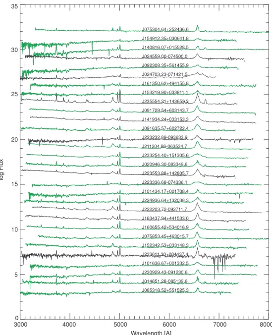
No. 4, 2009 EUV QSOs 3771 3000 4000 5000 6000 7000 8000 Wavelength [A] 0 5 10 15 20 25 30 35 log Flux J075304.64+252436.6 J154912.35+030641.8 J140816.07+015528.5 J024559.00-074500.0 J092308.35+561455.9 J024703.23-071421.5 J161350.62+494155.8 J153219.90+033811.1 J235554.21+143653.3 J091729.54+603143.7 J141934.24+033153.3 J091635.57+602722.4 J223232.89-093633.9 J211204.86-063534.7 J233254.40+151305.6 J020946.30-083349.6 J223553.88+142805.7 J223336.68-074336.1 J101434.17+001708.4 J224936.64+132038.3 J222203.72-092711.7 J163437.94+441533.0 J160655.42+534016.9 J075853.45+463015.7 J152342.53+033148.3 J233611.30+004437.4 J101636.67+001332.5 J230929.43-091230.6 J014651.28-085139.6 J085318.52+551525.3
Figure 8.Sample spectra of low-redshift UV-blue QSOs, labeled by theGALEXIAU identifier. Fluxes are scaled to have a constant offset at 6000–6500 Å. Spectra of extended objects are plotted in green/gray, and of pointlike sources in black. The order is FUV–NUV bluer to redder, top to bottom, but the spectral features, especially the slope, do not show any obvious trend with UV color.
(A color version of this figure is available in the online journal.)
and in more detail the relative amounts of absorption in the wavelength ranges sampled by theGALEXFUV and NUV filters atz≈2 vary according to the dust geometry and composition. For example, comparison of dust models in figure A.2 of Binette & Krongold (2008) suggests that a lower column density of the carbon crystalline dust screen (or an intrinsic SED steeper toward short wavelengths) may produce a higher FUV flux, and small grain dust (similar composition as MW dust, i.e., silicate and graphite grains, but grain sizes much smaller than MW dust and larger than nanodiamonds) would cause a significant depression of the observed-NUV flux but less reduction of the observed FUV at the redshift of our high-zUV-blue QSOs. This effect would be qualitatively consistent with the SED of our UV-blue QSOs. From broadband photometry alone, it is not possible to separate effects of dust absorption and intrinsic SED slope, therefore we can only speculate that the observed FUV– NUV colors in our sample are qualitatively compatible with
absorption from dust with grains differing from the MW dust (smaller grains), and possibly a steeper flux rise toward EUV. The question remains open as to what causes the extremely blue FUV–NUV colors, and whether these objects have known counterparts with similar properties, until UV spectroscopy can be obtained.
We have measured the emission lines of Civand Ciii(EW,
total flux, and full width (FW) at 10% of the peak flux above the local continuum) from the SDSS spectra. Typical errors are of the order of 10%. Lyαis generally too near the end of the optical spectra and could be measured only in 10 cases. The Ciii
line is free of absorptions but some QSOs have significant BAL and interstellar absorptions in the Civline. The emission line
properties do not correlate at all with the FUV–NUV color. The FUV–NUV color does correlate with theg−icolor, which may indicate that extinction is involved, and with redshift, although weakly, in the sense that higher redshift objects are more
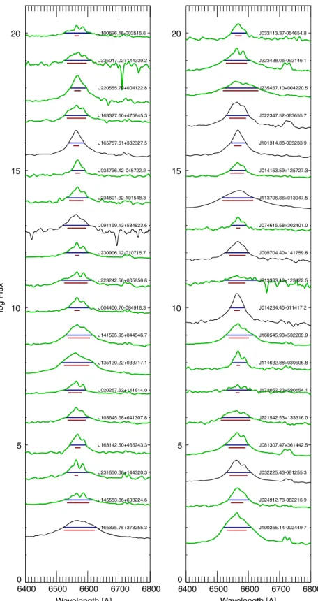
6400 6500 6600 6700 6800 Wavelength [A] 0 5 10 15 20 log Flux J100626.18-003515.6 J235017.02+144230.2 J220555.79+004122.8 J163327.60+475845.3 J165757.51+382327.5 J034736.42-045722.2 J234601.32-101548.3 J091159.13+584823.6 J230906.12-010715.7 J223242.56+005856.8 J004400.70-084916.3 J141505.95+044546.7 J135120.22+033717.1 J020257.62+141614.0 J103645.68+641307.8 J163142.50+465243.3 J231650.38+144320.3 J145553.86+603224.6 J165335.75+373255.3 6400 6500 6600 6700 6800 Wavelength [A] 0 5 10 15 20 J033113.37-054654.8 J223438.06-092146.1 J235457.10+004220.5 J022347.52-083655.7 J101314.88-005233.9 J014153.59+125727.3 J113706.86+013947.5 J074615.58+302401.0 J005704.40+141759.8 J213933.10+123422.5 J014234.40-011417.2 J160545.93+532209.9 J114632.88+030506.8 J172052.23+590154.1 J221542.53+133316.0 J081307.47+361442.5 J032225.43-081255.3 J024912.73-082216.9 J100255.14-002449.7
Figure 9.Hαline of about one-third of the low-zobjects (black: pointlike; green: extended sources). Profiles vary from very broad to narrow, to broad profiles with superimposed narrow components. The line width measured with our code (see the text) is shown with a blue horizontal line, the width from the SDSS pipeline with a red line (plotted lower for clarity). Fluxes (Fλ) are offset for clarity.
UV-blue (Figures5and15). This is what we would expect in the rest wavelengths below the Lyman limit, where the continuum is rising again. The Lyman discontinuity is larger for higher redshifts too, which is likely caused by where it lies between the NUV and u bandpasses. The emission line EW is larger for fainter FUV magnitudes, but scales more slowly than the
continuum flux. The line FW is higher for more luminous QSOs, based on their g-band magnitudes (rest-frame FUV). Flux and EW of Ciiiand Civlines correlate with the Lyman
discontinuity, but not the line FW. Thus, there is a connection between line emission and the EUV continuum. Figure15shows some of these correlations; the Spearman’sρ significance test
No. 4, 2009 EUV QSOs 3773
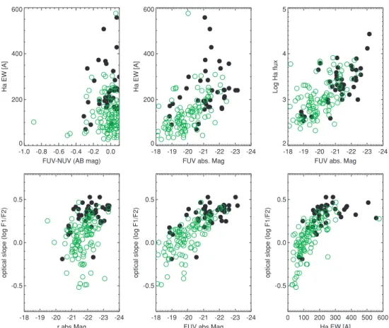
-1.0 -0.8 -0.6 -0.4 -0.2 0.0 FUV-NUV (AB mag) 0 200 400 600 Ha EW [A] -18 -19 -20 -21 -22 -23 -24 FUV abs. Mag 0 200 400 600 Ha EW [A] -18 -19 -20 -21 -22 -23 -24 FUV abs. Mag 2 3 4 5 Log Ha flux -18 -19 -20 -21 -22 -23 -24 r abs.Mag -0.5 0.0 0.5
optical slope (log F1/F2)
-18 -19 -20 -21 -22 -23 -24 FUV abs.Mag -0.5
0.0 0.5
optical slope (log F1/F2)
0 100 200 300 400 500 600 Ha EW [A]
-0.5 0.0 0.5
optical slope (log F1/F2)
Figure 10.Hαemission and optical spectral slopeFλ1(3500–3700 Å)/Fλ2(6000–6400 Å) of the low-redshift QSOs show correlation with the UV absolute magnitude, but not with the FUV–NUV color or optical absolute magnitude. Spectral slope, and to a lesser extent the Hαflux and EW, differ between pointlike (black dots) and extended (green/gray circles) samples. The Hαflux is in units of 10−17erg cm−2s−1. If we restrict the sample to redshiftz=0.15–0.25 (where Lyαis centered in the FUV filter) the correlations in the right and middle panels become tighter.
FUV NUV u g r i z 24 22 20 18 16 14 Magnitude [AB]
Figure 11.GALEXand SDSS magnitudes for the low-redshift sample, and median magnitudes as solid lines (black: pointlike; green: extended sources). Magnitudes are plotted at theλeffof each filter, on a logarithmic wavelength scale. Dashed lines are the median for the comparison sample of UV-normal QSOs. Lyαlies within the FUV channel for these objects and will contribute to the FUV–NUV color. In FUV–NUV the greatest difference is seen, consistent with our sample selection. For both UV-blue and UV-normal samples, we simply averaged all QSOs within the same redshift range. The number of objects across the redshift range however is distributed nonuniformly for each sample; if we eliminate the weight of the relative number of objects and combine median values in small redshift bins, the curves change very little, and the general trend is the same. Because average magnitudes vary with redshift, average properties of samples vary according to how the sample is defined. Therefore, small differences should not be overinterpreted but we believe that the general trend is robust. FUV NUV u g r i z 24 22 20 18 16 Magnitude [AB] Red QSO Median Normal QSOs
Figure 12.GALEXand SDSS average magnitudes for the high-redshift sample. The Lyman limit lies between the NUV andubands in this redshift range. The line is the median values for each and the dotted line is the one discrepant QSO with a very red optical spectrum. The dashed line is the average from a sample of UV-normal QSOs within the same redshift range (1.7–2.4). Photometry of each object has been corrected for interstellar extinction usingE(B−V) given in Table1; the same correction was applied to the UV-normal sample before deriving the average. A plot without extinction correction applied is qualitatively very similar, shifted slightly toward fainter values, especially in UV, but the relative differences remain the same. Magnitudes are plotted at theλeffof each filter, on a logarithmic wavelength scale.
1000 1500 2000 2500 3000 Restframe Wavelength [A]
5 10 15 20 25 30 log Flux
High redshift sample: optical spectra
J075627.72+205415.1 J025221.08-085516.0 J161821.57+492603.0 J222323.21-084740.5 J145645.30+595436.2 J211858.56-063027.3 J082337.98+455621.4 J003505.58-103536.4 J230724.98+000958.0 J113638.68+011031.5 J155013.52+033744.6 J233139.76+010428.7 J090814.51+550701.6 J015229.22-083640.0 J020419.29+143929.2 J082616.05+502049.5 J005408.42-094637.1 J145055.62+015419.0 J141807.07+050431.3 J085344.92+565337.9 J084658.13+465011.4
Figure 13.Optical spectra of the high-zsample, plotted in the rest-frame wavelength. The spectra (inFλ) are scaled so to have a constant offset at 2000–2500 Å. They are ordered (top to bottom) by FUV–NUV (bluer to redder), and labeled with theirGALEXIAU identifier. Only for a few objects Lyαis included in the spectrum, at the edge of the observed range.
gives a probability of correlation (clockwise from top left) of 99%, 94%, 58%, and 99%.
While the dust absorption affects more the continuum, the ionization would be reflected by the line ratios. Binette & Krongold (2008, and references therein) discuss also the effects of shock ionization versus photoionization. It is interesting that their models show low Civand Nvrelative to Lyα, compared
with UV-normal QSOs. We measured Lyα+N v and C iv in
our high-redshift UV QSOs where possible (10 cases). The line flux ratios may be useful diagnostic since shocks may not be related to the continuum. Therefore, we also examined SDSS spectra of UV-normal QSOs in the same redshift range and compared their line strength with the UV-blue sample. We extracted spectroscopically confirmed QSOs in the same redshift rangez=1.7–2.5, but with FUV–NUV>0.1, from our master catalog of matched sources. We found 420 objects, compared with our 21 with FUV–NUV < 0.1. We imposed the same error cuts in FUV, which unfavors the red (normal) QSOs, so the ratio (5%) is a lower limit for the fraction of UV-blue QSOs compared with normal ones. The relative numbers however may be highly biased because the SDSS spectral targets were chosen with criteria not related to our UV selection. We measured the same line ratio only for the UV-normal comparison objects with
z=2.2–2.5, where Lyαis included in the optical spectra. The measurements are shown in Figure16, where a linear fit is also shown; the formal probability of correlation is over 99%. The average line ratios for the UV-blue and UV-normal samples are
given in Table4. The average is 5.2 for our UV-blue sample and 3.7 for our normal comparison sample. The collisional model predicts a ratio of∼6.7, and the photoionization model 1.8. In one of our UV QSOs the ratio Lyα+Nv/Civis about 10, while
Ton 34 has a ratio of 8.7. This bears out the similarity with Ton 34, and a dominance of collisional ionization, compared with UV-normal QSOs.
5. CONCLUSIONS AND SUMMARY
We analyzed 171 spectroscopically confirmed QSOs with FUV–NUV color bluer than 0.1, extracted from theGALEXMIS survey with complementary SDSS optical data. Most of these objects have redshift<0.5, and we speculate that Lyαemission enhanced up to a factor of 3 with respect to average templates, may explain the observed colors. Their optical properties are similar to those of UV-normal QSOs. Both photometric and emission line properties differ between pointlike and extended sources, reflecting the contribution from the host galaxy in the latter. The slope of their optical spectra and the strength of Hα (flux and EW) correlate (increase) with intrinsic UV luminosity. Lyα goes through the GALEX FUV band in the redshift range of these objects, between 0.1 and 0.5, therefore the resulting effect on the broadband FUV magnitude is a combination of the line intensity and the filter’s transmission curve. A restricted subsample with redshift around 0.2 (where Lyαis at the peak of the filter’s transmission) seems to show
No. 4, 2009 EUV QSOs 3775
Figure 14.Visible spectra of the high-redshift QSOs. Top: fluxes (Fλ) have been scaled to a common value in the range 2000–2500 Å. The “hottest” spectrum is the hot star, misclassified by the SDSS pipeline as a QSO of redshiftz=2.7: in the observed wavelength scale, the absorptions are the Balmer lines. Vertical dotted lines mark Lyαand C IVλ1550 positions. The cyan spectrum is the standard QSO template. The extremely red spectrum is discussed separately (Figure4). Bottom: averaged optical spectra of our UV-blue sample, and UV-normal comparison sample in the same redshift range. The Civdoublet is different. For Lyαno conspicuous
difference is seen, but this line is available only for few “UV-blue” QSOs, making the comparison not significant.
tighter correlations but it is statistically insufficient to support conclusions. The UV luminosity is brighter (∼0.5–1 mag on average) than that of our UV-normal comparison sample, the difference being larger in FUV and for the pointlike objects (Figures6and11).
Our sample of UV-blue QSOs also includes 21 objects with redshift between 1.7 and 2.6. Their photometric errors are generally large, the combined FUV–NUV 1σerrors are between 0.1 and 0.37 mag, but our FUV–NUV selection limit (FUV– NUV <0.1) is bluer than typical QSO colors at this redshift by more than 0.5 mag, and the observed FUV–NUV colors are bluer than the typical color by up to 1 mag or more (Figure1). For these UV-blue QSOs at higher redshift, we speculate that
a combination of unusually strong absorption inGALEX-NUV (rest-frame∼600–900 Å) and EUV-steeply rising flux (GALEX
FUV ∼ rest-frame 450–590 Å) may explain the FUV–NUV color. This is suggested by two facts. First, ad hoc templates with flux rising toward rest-frame EUV more steeply than in canonical templates, produce observed FUV–NUV colors bluer than the average template (Figure2), but still redder than our selection limit by 0.2 mag and redder than most of our UV-blue sample by up to 1 mag. Second, comparison with average SED of a UV-normal QSO sample, shows the NUV luminosity of the UV-blue sample to be fainter, suggesting absorption in the observed NUV. Dust with composition similar to the typical MW dust but smaller grains and carbon crystalline nanosized grains
Figure 15.Quantities which show trends with UV data in the high-redshift sample. The Lyman break value is the mean of the twoGALEXmagnitudes minus the mean of the five SDSS magnitudes. The dotted lines are linear fits to the points. The red QSO (see Figure4) is very discrepant in the lower two plots and is off-scale and not fitted by the line. FUV–NUV is in AB magnitudes. The FW (in Å) plotted in the upper-right panel is measured at 10% of the peak flux above the local continuum, by line profile fitting.
Figure 16.Ratio of Lyα+Nvto Civemission for the UV sample (circles) and a comparison sample with similar redshift but FUV–NUV>0.1 (filled dots). Although
the sample is very limited, the UV-blue QSOs tend to have a higher ratio, suggestive that collisions may be more relevant. The line is a linear fit.
(nanodiamonds) would cause absorption in the observed NUV band, according to the models of Binette & Krongold (2008), which may qualitatively account for the observed FUV–NUV colors. UV spectroscopy is needed to pinpoint the cause for the FUV–NUV color of these objects. The Lyαto Civratio is
stronger in the optical spectra of the UV-blue QSOs than in the UV-normal comparison sample (at the>95% confidence level from the Kolmogorov–Smirnov test, although both samples are very small, see Figure16), suggesting collisional ionization to be more relevant in the UV-blue QSOs.
The group of UV QSOs atz∼ 2 may probe a particularly relevant phase of galaxy formation, tightly connected with the formation of the massive central black hole. In current QSO/
Spheroid co-evolution models (e.g., Granato et al.2004), the power of the central QSO rises almost exponentially and quickly stops the star formation process. During the previous phase it is strongly dust enshrouded and not visible except in X rays. A phase of decreasing (but still significant) extinction follows, and finally a shining phase until the fuel is consumed. A quick transition is expected between dust extinguished and