esys-Escript User’s Guide: Solving Partial Differential Equations with Escript and Finley Release - 4.1 (r5754)

(1)

esys-Escript

User’s Guide:

Solving Partial Differential Equations

with Escript and Finley

Release - 4.1

(r5754)

Lutz Gross

et al.

(Editor)

24 July 2015

Centre for Geoscience Computing (GeoComp)

School of Earth Sciences

The University of Queensland

Brisbane, Australia

(2)

Primary Business: Queensland, Australia Licensed under the Open Software License version 3.0 http://www.opensource.org/licenses/osl-3.0.php Development until 2012 by Earth Systems Science Computational Center (ESSCC)

Development 2012-2013 by School of Earth Sciences

Development from 2014 by Centre for Geoscience Computing (GeoComp)

This work is supported by the AuScope National Collaborative Research Infrastructure Strategy, the Queensland State Government and The University of Queensland.

(3)

Guide to Documentation

Documentation foresys.escriptcomes in a number of parts. Here is a rough guide to what goes where.

install.pdf “Installation guide for esys-Escript”: Instructions for compiling escript for your system from its source code. Also briefly covers installing.deb pack-ages for Debian and Ubuntu.

cookbook.pdf “TheescriptCOOKBOOK”: An introduction toescriptfor new users from a geophysics perspective.

user.pdf “esys-EscriptUser’s Guide: Solving Partial Differential Equations with Escript and Finley”: Covers mainescriptconcepts.

inversion.pdf “esys.downunder: Inversion withescript”: Explanation of the inversion toolbox forescript.

sphinx api directory Documentation forescript Pythonlibraries.

escript examples(.tar.gz)/(.zip) Full example scripts referred to by other parts of the documentation. doxygen directory Documentation for C++ libraries (mostly only of interest for developers).

(4)

Abstract

esys.escriptis apython-based environment for implementing mathematical models, in particular those based on coupled, non-linear, time-dependent partial differential equations. It consists of five major components:

• esys.escriptcore library

• finite element solversesys.finley,esys.dudley,esys.ripley, andesys.speckley(which use fast vendor-supplied solvers or the includedPASOlinear solver library)

• the meshing interfaceesys.pycad • a model library

• an inversion module.

Allesys.escriptmodules should work under bothpython2 andpython3, see AppendixE. The current version supports parallelization throughMPIfor distributed memory,OpenMP for shared memory on CPUs, as well asCUDAfor some GPU-based solvers.

This release comes with some significant changes and new features. Please see AppendixBfor a detailed list. If you use this software in your research, then we would appreciate (but do not require) a citation. Some relevant references can be found in AppendixD.

(5)

Researchers and Developers

Escript is the product of years of work by many people. The active researchers for the current release series (4.x) are listed here in alphabetical order. While development is collaborative, each person is listed with some of their major contributions — this list is not exhaustive. Personel for previous release series are listed in an appendix of

the user guide.

Cihan Altinay esys.weipavisualisation package, SCons build system rework, esys.ripleyand CUDA solvers.

Joel Fenwick Lazy evaluation, maintenance of escript module, release wrangler. Lutz Gross Patriarch, technical lead, solvers, large chunks of the original code. Jaco du Plessis Symbolic toolbox, GMSH reader MPI implementation, DC resistivity. Simon Shaw esys.speckleymodule, release help, large cluster improvements.

(6)

(7)

11.4 Classes . . . 142 11.4.1 Symbol class . . . 142 11.4.2 Evaluator class . . . 143 11.4.3 NonlinearPDE class . . . 144 11.4.4 Symconsts class . . . 144 A Einstein Notation 145 B Changes from previous releases 147 C Escript researchers and developers by release 153 D Escript references 155 E Python3 Support 157 E.1 Impact on scripts . . . 157

Index 159

Bibliography 163

(10)

(11)

CHAPTER

ONE

Tutorial: Solving PDEs

1.1 Installation

To downloadescriptand friends, please visithttps://launchpad.net/escript-finley. The web site offers binary distributions for some platforms, source code, documentation including information about the instal-lation process, as well as a way to ask questions.

1.2 The First Steps

In this chapter we give an introduction how to useesys.escriptto solve a partial differential equation (PDE). We assume you are at least a little familiar withpython. The knowledge presented in thepythontutorial athttps: //docs.python.org/2/tutorial/is more than sufficient.

The PDE we wish to solve is the Poisson equation

−∆u=f (1.1)

for the solutionu. The functionf is the given right hand side. The domain of interest, denoted byΩ, is the unit square

Ω = [0,1]2={(x0;x1)|0≤x0≤1and0≤x1≤1} (1.2)

The domain is shown in Figure1.1.

x x 0 1 (0, 0) (1, 1) n

FIGURE1.1: DomainΩ = [0,1]2with outer normal fieldn.

∆denotes the Laplace operator, which is defined by

∆u= (u,0),0+ (u,1),1 (1.3)

(12)

where, for any functionuand any directioni,u,idenotes the partial derivative ofuwith respect toi.1 _Basically, in the subindex of a function, any index to the right of the comma denotes a spatial derivative with respect to the index. To get a more compact form we will writeu,ij= (u,i),jwhich leads to

∆u=u,00+u,11= 2

X i=0

u,ii (1.4)

We often find that use of nestedP

symbols makes formulas cumbersome, and we use the more compact Einstein summation convention. This drops the P

sign and assumes that a summation is performed over any repeated index. For instance we write

xiyi = 2 X i=0 xiyi (1.5) xiu,i= 2 X i=0 xiu,i (1.6) u,ii= 2 X i=0 u,ii (1.7) xijui,j = 2 X j=0 2 X i=0 xijui,j (1.8) (1.9) With the summation convention we can write the Poisson equation as

−u,ii= 1 (1.10)

wheref = 1in this example.

On the boundary of the domainΩthe normal derivativeniu,iof the solutionushall be zero, i.e.ushall fulfill the homogeneous Neumann boundary condition

niu,i= 0. (1.11)

n= (ni)denotes the outer normal field of the domain, see Figure1.1. Remember that we are applying the Einstein summation convention , i.e.niu,i=n0u,0+n1u,1.2 The Neumann boundary condition of Equation (1.11) should

be fulfilled on the setΓN which is the top and right edge of the domain:

ΓN ={(x0;x1)∈Ω|x0= 1orx1= 1} (1.12)

On the bottom and the left edge of the domain which is defined as

ΓD={(x0;x1)∈Ω|x0= 0orx1= 0} (1.13)

the solution shall be identical to zero:

u= 0. (1.14)

This kind of boundary condition is called a homogeneous Dirichlet boundary condition. The partial differential equation in Equation (1.10) together with the Neumann boundary condition Equation (1.11) and Dirichlet boundary condition in Equation (1.14) form a so-called boundary value problem (BVP) for the unknown functionu.

1_{You may be more familiar with the Laplace operator being written as}_∇2_{, and written in the form}

∇2_u₌_∇t_{· ∇}_u₌∂2u ∂x2 0 +∂ 2_u ∂x2 1 and Equation (1.1) as −∇2_u₌_f 2_{Some readers may familiar with the notation}∂u

∂n=niu,ifor the normal derivative.

(13)

Element Node

FIGURE1.2: Mesh of4×4elements on a rectangular domain. Here each element is a quadrilateral and described by four nodes, namely the corner points. The solution is interpolated by a bi-linear polynomial.

In general the BVP cannot be solved analytically and numerical methods have to be used to construct an approximation of the solutionu. Here we will use the finite element method (FEM). The basic idea is to fill the domain with a set of points called nodes. The solution is approximated by its values on the nodes. Moreover, the domain is subdivided into smaller sub-domains called elements. On each element the solution is represented by a polynomial of a certain degree through its values at the nodes located in the element. The nodes and their connection through elements is called a mesh. Figure1.2shows an example of a FEM mesh with four elements in thex0and four elements in thex1direction over the unit square. For more details we refer the reader to the

literature, for instance Reference [40,5].

Theesys.escriptsolver we want to use to solve this problem is embedded into the pythoninterpreter language. So you can solve the problem interactively but you will learn quickly that it is more efficient to use scripts which you can edit with your favorite editor. To enter the escript environment, use therun-escript command3_:

run-escript

which will pass you on to thepythonprompt

Python 2.7.6 (default, Mar 22 2014, 15:40:47) [GCC 4.8.2] on linux2

Type "help", "copyright", "credits" or "license" for more information. >>>

Here you can use all availablepythoncommands and language features4, for instance

>>> x=2+3

>>> print("2+3=",x) 2+3= 5

We refer to thepythonuser’s guide if you are not familiar withpython.

esys.escriptprovides the classPoissonto define a Poisson equation. (We will discuss a more general form of a PDE that can be defined through theLinearPDEclass later.) The instantiation of aPoissonclass ob-ject requires the specification of the domainΩ. Inesys.escripttheDomainclass objects are used to describe the geometry of a domain but it also contains information about the discretization methods and the actual solver which is used to solve the PDE. Here we are using the FEM libraryesys.finley. The following statements create theDomainobjectmydomainfrom theesys.finleyfunctionRectangle:

from esys.finley import Rectangle

mydomain = Rectangle(l0=1.,l1=1.,n0=40, n1=20)

3_run-escript _{is not available under Windows.} _{If you run under Windows you can just use the} _python _{command and the}

OMP NUM THREADSenvironment variable to control the number of threads.

4_{Throughout our examples, we use the python 3 form of print. That is, print(1) instead of print 1.}

(14)

In this case the domain is a rectangle with the lower left corner at point (0,0) and the upper right corner at (l0,l1) = (1,1). The argumentsn0andn1define the number of elements inx0andx1-direction respectively.

For more details onRectangleand otherDomaingenerators see Chapter7, Chapter8, and Chapter9. The following statements define thePoissonclass object mypdewith domainmydomainand the right hand sidef of the PDE to constant1:

from esys.escript.linearPDEs import Poisson mypde = Poisson(mydomain)

mypde.setValue(f=1)

We have not specified any boundary condition but thePoissonclass implicitly assumes homogeneous Neuman boundary conditions defined by Equation (1.11). With this boundary condition the BVP we have defined has no unique solution. In fact, with any solutionuand any constantCthe functionu+Cbecomes a solution as well. We have to add a Dirichlet boundary condition. This is done by defining a characteristic function which has positive values at locationsx = (x0, x1)where Dirichlet boundary condition is set and0 elsewhere. In our case ofΓD

defined by Equation (1.13), we need to construct a functiongammaDwhich is positive for the casesx0 = 0or

x1= 0. To get an objectxwhich contains the coordinates of the nodes in the domain use

x=mydomain.getX()

The methodgetXof theDomain mydomaingives access to locations in the domain defined bymydomain. The objectxis actually aDataobject which will be discussed in Chapter3in more detail. What we need to know here is thatxhas rank (number of dimensions) and a shape (list of dimensions) which can be viewed by calling thegetRankandgetShapemethods:

print("rank ",x.getRank(),", shape ",x.getShape())

This will print something like

rank 1, shape (2,)

TheDataobject also maintains type information which is represented by theFunctionSpaceof the object. For instance

print(x.getFunctionSpace())

will print

Finley_Nodes [ContinuousFunction(domain)] on FinleyMesh

which tells us that the coordinates are stored on the nodes of (rather than on points in the interior of) a Finley mesh. To get thex0coordinates of the locations we use the statement

x0=x[0]

Objectx0is again aDataobject now with rank0and shape(). It inherits theFunctionSpacefromx: print(x0.getRank(), x0.getShape(), x0.getFunctionSpace())

will print

0 () Finley_Nodes [ContinuousFunction(domain)] on FinleyMesh

We can now construct a functiongammaDwhich is only non-zero on the bottom and left edges of the domain with from esys.escript import whereZero

gammaD=whereZero(x[0])+whereZero(x[1])

whereZero(x[0])creates a function which equals1 wherex[0]is (almost) equal to zero and 0 else-where. Similarly, whereZero(x[1]) creates a function which equals1 wherex[1]is equal to zero and0 elsewhere. The sum of the results ofwhereZero(x[0]) andwhereZero(x[1])gives a function on the domainmydomainwhich is strictly positive wherex0orx1is equal to zero. Note thatgammaDhas the same

rank , shape andFunctionSpacelikex0used to define it. So from

print(gammaD.getRank(), gammaD.getShape(), gammaD.getFunctionSpace())

one gets

0 () Finley_Nodes [ContinuousFunction(domain)] on FinleyMesh

(15)

An additional parameterqof thesetValuemethod of thePoissonclass defines the characteristic function of the locations of the domain where the homogeneous Dirichlet boundary condition is set. The complete definition of our example is now:

from esys.escript.linearPDEs import Poisson x = mydomain.getX()

gammaD = whereZero(x[0])+whereZero(x[1]) mypde = Poisson(domain=mydomain)

mypde.setValue(f=1,q=gammaD)

The first statement imports thePoissonclass definition from theesys.escript.linearPDEsmodule. To get the solution of the Poisson equation defined bymypdewe just have to call itsgetSolutionmethod.

Now we can write the script to solve our Poisson problem from esys.escript import *

from esys.escript.linearPDEs import Poisson

# generate domain:

# define characteristic function of GammaˆD

x = mydomain.getX()

gammaD = whereZero(x[0])+whereZero(x[1])

# define PDE and get its solution u

mypde = Poisson(domain=mydomain) mypde.setValue(f=1, q=gammaD) u = mypde.getSolution()

The question is what we do with the calculated solutionu. Besides postprocessing, e.g. calculating the gradient or the average value, which will be discussed later, plotting the solution is one of the things you might want to do.esys.escriptoffers two ways to do this, both based on external modules or packages. The first option is using thematplotlibmodule which allows plotting 2D results relatively quickly from within thepythonscript, see [16]. However, there are limitations when using this tool, especially for large problems and when solving three-dimensional problems. Therefore,esys.escriptprovides functionality to export data as files which can subsequently be read by third-party software packages such asMayavi2[18] orVisIt[36].

1.2.1 Plotting Using

matplotlib

Thematplotlibmodule provides a simple and easy-to-use way to visualize PDE solutions (or otherData ob-jects). To hand over data fromesys.escripttomatplotlibthe values need to be mapped onto a rectangular grid. We will make use of thenumpymodule for this.

First we need to create a rectangular grid which is accomplished by the following statements: import numpy

x_grid = numpy.linspace(0., 1., 50) y_grid = numpy.linspace(0., 1., 50)

x_gridis an array defining the x coordinates of the grid whiley_griddefines the y coordinates of the grid. In this case we use50points over the interval[0,1]in both directions.

Now the values created byesys.escriptneed to be interpolated to this grid. We will use thematplotlib mlab.griddatafunction to do this. Spatial coordinates are easily extracted as alistby

x=mydomain.getX()[0].toListOfTuples() y=mydomain.getX()[1].toListOfTuples()

In principle we can apply the sametoListOfTuplesmethod to extract the values from the PDE solutionu. However, we have to make sure that theDataobject we extract the values from uses the sameFunctionSpace as we have used when extractingxandy. We apply theinterpolationtoubefore extraction to achieve this:

z=interpolate(u, mydomain.getX().getFunctionSpace())

The values inzare the values at the points with the coordinates given byxandy. These values are interpolated to the grid defined byx_gridandy_gridby using

import matplotlib

z_grid = matplotlib.mlab.griddata(x, y, z, xi=x_grid, yi=y_grid)

(16)

0.0 0.2 0.4 0.6 0.8 1.0 0.0 0.2 0.4 0.6 0.8 1.0

FIGURE1.3: Visualization of the Poisson Equation Solution forf= 1usingmatplotlib

Nowz_gridgives the values of the PDE solutionuat the grid which can be plotted usingcontourf:

matplotlib.pyplot.contourf(x_grid, y_grid, z_grid, 5) matplotlib.pyplot.savefig("u.png")

Here we use 5 contours. The last statement writes the plot to the fileu.pngin the PNG format. Alternatively, one can use

matplotlib.pyplot.contourf(x_grid, y_grid, z_grid, 5) matplotlib.pyplot.show()

which gives an interactive browser window.

Now we can write the script to solve our Poisson problem from esys.escript import *

import numpy

import matplotlib

import pylab

# generate domain:

x = mydomain.getX()

mypde = Poisson(domain=mydomain) mypde.setValue(f=1,q=gammaD) u = mypde.getSolution()

# interpolate u to a matplotlib grid:

x_grid = numpy.linspace(0.,1.,50) y_grid = numpy.linspace(0.,1.,50) x=mydomain.getX()[0].toListOfTuples() y=mydomain.getX()[1].toListOfTuples() z=interpolate(u,mydomain.getX().getFunctionSpace()).toListOfTuples() z_grid = matplotlib.mlab.griddata(x,y,z,xi=x_grid,yi=y_grid )

# interpolate u to a rectangular grid:

matplotlib.pyplot.contourf(x_grid, y_grid, z_grid, 5) matplotlib.pyplot.savefig("u.png")

(17)

FIGURE1.4: Visualization of the Poisson Equation Solution forf= 1

The entire code is available aspoisson_matplotlib.pyin the example directory. You can run the script using theescriptenvironment

run-escript poisson_matplotlib.py

This will create a file calledu.png, see Figure1.3. For details on the usage of thematplotlibmodule we refer to the documentation [16].

As pointed out,matplotlibis restricted to the two-dimensional case and should be used for small problems only. It can not be used underMPIas thetoListOfTuplesmethod is not safe underMPI5_.

1.2.2 Visualization using export files

As an alternative tomatplotlib,escriptsupports exporting data toVTKandSILOfiles which can be read by visualization tools such asMayavi2[18] andVisIt[36]. This method isMPIsafe and works with large 2D and 3D problems.

To write the solutionuof the Poisson problem in theVTKfile format to the fileu.vtuone needs to add: from esys.weipa import saveVTK

saveVTK("u.vtu", sol=u)

This file can then be opened in aVTKcompatible visualization tool where the solution is accessible by the name sol. Similarly,

from esys.weipa import saveSilo saveSilo("u.silo", sol=u)

will writeuto aSILOfile if escript was compiled with support for LLNL’sSILOlibrary. The Poisson problem script is now

from esys.escript import _*

from esys.weipa import saveVTK

# generate domain:

5_{The phrase ’safe under}_MPI_{’ means that a program will produce correct results when run on more than one processor under}_MPI_.

(18)

x

0

x

1

n

T

_ref

FIGURE1.5: Temperature Diffusion Problem with Circular Heat Source

x = mydomain.getX()

mypde = Poisson(domain=mydomain) mypde.setValue(f=1,q=gammaD) u = mypde.getSolution()

# write u to an external file

saveVTK("u.vtu",sol=u)

The entire code is available aspoisson_vtk.pyin the example directory.

You can run the script using theescriptenvironment and visualize the solution usingMayavi2: run-escript poisson_vtk.py

mayavi2 -d u.vtu -m Surface The result is shown in Figure1.4.

1.3 The Diffusion Problem

1.3.1 Outline

In this section we will discuss how to solve a time-dependent temperature diffusion PDE for a given block of material. Within the block there is a heat source which drives the temperature diffusion. On the surface, energy can radiate into the surrounding environment. Figure1.5shows the configuration.

In the next Section1.3.2 we will present the relevant model. A time integration scheme is introduced to calculate the temperature at given time nodest(n). We will see that at each time step a Helmholtz equation must be solved. The implementation of a Helmholtz equation solver will be discussed in Section1.3.3. In Section1.3.4 this solver is used to build a solver for the temperature diffusion problem.

1.3.2 Temperature Diffusion

The unknown temperatureT is a function of its location in the domain and timet >0. The governing equation in the interior of the domain is given by

ρcpT,t−(κT,i),i=qH (1.15)

whereρcp andκare given material constants. In case of a composite material the parameters depend on their location in the domain. qH is a heat source (or sink) within the domain. We are using the Einstein summation convention as introduced in Chapter1.2. In our case we assumeqHto be equal to a constant heat production rate qc_{on a circle or sphere with center}_xc_{and radius}_r_{, and}₀_elsewhere:

qH(x, t) =

qc _if_kx₋_xc_{k ≤}_r

0 else (1.16)

(19)

for allxin the domain and timet >0.

On the surface of the domain we specify a radiation condition which prescribes the normal component of the fluxκT,ito be proportional to the difference of the current temperature to the surrounding temperatureTref:

κT,ini=η(Tref −T) (1.17)

ηis a given material coefficient depending on the material of the block and the surrounding medium.niis thei-th component of the outer normal field at the surface of the domain.

To solve the time-dependent Equation (1.15) the initial temperature at time t = 0has to be given. Here we assume that the initial temperature is the surrounding temperature:

T(x,0) =Tref (1.18)

for allxin the domain. Note that the initial conditions satisfy the boundary condition defined by Equation (1.17). The temperature is calculated at discrete time nodest(n)_where_t(0)_{= 0}_and_t(n)₌_t(n−1)₊_h_{, where}_{h >}₀

is the step size which is assumed to be constant. In the following, the upper index(n)refers to a value at timet(n)_.

The simplest and most robust scheme to approximate the time derivative of the temperature is the backward Euler scheme. The backward Euler scheme is based on the Taylor expansion ofTat timet(n)_:

T(n)≈T(n−1)+T_,t(n)(t(n)−t(n−1)) =T(n−1)+h·T_,t(n) (1.19) This is inserted into Equation (1.15). By separating the terms att(n)_and_t(n−1)_{one gets for}_n_{= 1,}_2,₃_{. . .}

ρcp h T (n)₋_(κT(n) ,i ),i=qH+ ρcp h T (n−1) _(1.20)

whereT(0)₌_Tref _{is taken form the initial condition given by Equation (1.18). Together with the natural boundary}

condition

κT_,i(n)ni=η(Tref −T(n)) (1.21)

taken from Equation (1.17) this forms a boundary value problem that has to be solved for each time step. As a first step to implement a solver for the temperature diffusion problem we will implement a solver for the boundary value problem that has to be solved at each time step.

1.3.3 Helmholtz Problem

The partial differential equation to be solved forT(n)_{has the form}

ωT(n)−(κT_,i(n)),i=f (1.22) and we set ω=ρcp h andf =qH+ ρcp h T (n−1)_. _(1.23)

Withg=ηTref the radiation condition defined by Equation (1.21) takes the form

κT_,i(n)ni=g−ηT(n)onΓ (1.24) The partial differential Equation (1.22) together with boundary conditions of Equation (1.24) is called the Helmholtz equation.

We want to use theLinearPDEclass provided byesys.escriptto define and solve a general linear, steady, second order PDE such as the Helmholtz equation. For a single PDE theLinearPDEclass supports the following form:

−(Ajlu,l),j+Du=Y (1.25)

where we show only the coefficients relevant for the problem discussed here. For the general form of a single PDE see Equation (4.1). The coefficients A andY have to be specified through Data objects in the general FunctionSpaceon the PDE or objects that can be converted into suchDataobjects. A is a rank-2Data object andDandY are scalar. The following natural boundary conditions are considered onΓ:

njAjlu,l+du=y . (1.26)

(20)

Notice that the coefficientAis the same as in the PDE Equation (1.25). The coefficientsdandyare each a scalar Dataobject in the boundaryFunctionSpace. Constraints for the solution prescribe the value of the solution at certain locations in the domain. They have the form

u=rwhereq >0 (1.27)

Both r andq are a scalar Data object whereq is the characteristic function defining where the constraint is applied. The constraints defined by Equation (1.27) override any other condition set by Equation (1.25) or Equa-tion (1.26). ThePoissonclass of theesys.escript.linearPDEsmodule, which we have already used in Chapter1.2, is in fact a subclass of the more generalLinearPDEclass. Theesys.escript.linearPDEs module provides aHelmholtzclass but we will make direct use of the generalLinearPDEclass.

By inspecting the Helmholtz equation (1.22) and boundary condition (1.24), and substitutinguforT(n)_{, we}

can easily assign values to the coefficients in the general PDE of theLinearPDEclass: Aij =κδij D=ω Y =f

d=η y=g (1.28)

δijis the Kronecker symbol defined byδij = 1fori=jand0otherwise. Undefined coefficients are assumed to be not present.6In this diffusion example we do not need to define a characteristic functionqbecause the boundary conditions we consider in Equation (1.24) are just the natural boundary conditions which are already defined in the LinearPDEclass (shown in Equation (1.26)).

The Helmholtz equation can be set up the following way7:

mypde=LinearPDE(mydomain)

mypde.setValue(A=kappa*kronecker(mydomain),D=omega,Y=f,d=eta,y=g) u=mypde.getSolution()

where we assume thatmydomainis aDomainobject andkappa,omega,eta, andgare given scalar values typically floator Data objects. ThesetValue method assigns values to the coefficients of the general PDE. ThegetSolutionmethod solves the PDE and returns the solution uof the PDE.kroneckeris an esys.escriptfunction returning the Kronecker symbol.

The coefficients can be set by several calls tosetValuein arbitrary order. If a value is assigned to a coefficient several times, the last assigned value is used when the solution is calculated:

mypde = LinearPDE(mydomain)

mypde.setValue(A=kappa*kronecker(mydomain), d=eta) mypde.setValue(D=omega, Y=f, y=g)

mypde.setValue(d=2*eta) # overwrites d=eta

u=mypde.getSolution()

In some cases the solver of the PDE can make use of the fact that the PDE is symmetric. A PDE is called symmetric if

Ajl=Alj . (1.29)

Note thatDanddmay have any value and the right hand sidesY,yas well as the constraints are not relevant. The Helmholtz problem is symmetric. TheLinearPDEclass provides the methodcheckSymmetryto check if the given PDE is symmetric.

mypde.setValue(A=kappa*kronecker(mydomain), d=eta)

print(mypde.checkSymmetry()) # returns True

mypde.setValue(B=kronecker(mydomain)[0])

print(mypde.checkSymmetry()) # returns False

mypde.setValue(C=kronecker(mydomain)[0])

print(mypde.checkSymmetry()) # returns True

Unfortunately, callingcheckSymmetryis very expensive and is only recommended for testing and debugging purposes. ThesetSymmetryOnmethod is used to declare a PDE symmetric:

6_{There is a difference in}_esys.escript_{for a coefficient to be not present and set to zero. Since in the former case the coefficient is not} processed, it is more efficient to leave it undefined instead of assigning zero to it.

7_{Note that this is not a complete code. The full source code can be found in “helmholtz.py”.}

(21)

mypde.setValue(A=kappa*kronecker(mydomain)) mypde.setSymmetryOn()

Now we want to see how we actually solve the Helmholtz equation on a rectangular domain of lengthl0= 5and

heightl1 = 1. We choose a simple test solution such that we can verify the returned solution against the exact

answer. Actually, we takeT =x0 (hereqH = 0) and then calculate the right hand side termsf andgsuch that the test solution becomes the solution of the problem. If we assumeκas being constant, an easy calculation shows that we have to choosef =ω·x0. On the boundary we getκniu,i=κn0. Thus we have to setg=κn0+ηx0.

The following scripthelmholtz.pywhich is available in the example directory implements this test problem using theesys.finleyPDE solver:

from esys.escript.linearPDEs import LinearPDE

# set some parameters

kappa=1. omega=0.1 eta=10.

# generate domain

mydomain = Rectangle(l0=5., l1=1., n0=50, n1=10)

# open PDE and set coefficients

mypde=LinearPDE(mydomain) mypde.setSymmetryOn() n=mydomain.getNormal() x=mydomain.getX() mypde.setValue(A=kappa*kronecker(mydomain), D=omega,Y=omega*x[0], \ d=eta, y=kappa*n[0]+eta*x[0])

# calculate error of the PDE solution

u=mypde.getSolution()

print("error is ",Lsup(u-x[0])) saveVTK("x0.vtu", sol=u)

To visualize the solution ‘x0.vtu’ you can use the command mayavi2 -d x0.vtu -m Surface

and it is easy to see that the solutionT =x0is calculated.

The script is similar to the script poisson.pydiscussed in Chapter 1.2. mydomain.getNormal() returns the outer normal field on the surface of the domain. The function Lsup is imported by the from esys.escript import * statement and returns the maximum absolute value of its argument. The error shown by the print statement should be in the order of 10−7_{. As piecewise bi-linear interpolation is used by}

esys.finleyto approximate the solution, and our solution is a linear function of the spatial coordinates, one might expect that the error would be zero or in the order of machine precision (typically≈10−15). However most PDE packages use an iterative solver which is terminated when a given tolerance has been reached. The default tolerance is10−8. This value can be altered by using thesetTolerancemethod of theLinearPDEclass.

1.3.4 The Transition Problem

Now we are ready to solve the original time-dependent problem. The main part of the script is the loop over time twhich takes the following form:

t=0 T=Tref

mypde=LinearPDE(mydomain)

mypde.setValue(A=kappa*kronecker(mydomain), D=rhocp/h, d=eta, y=eta*Tref)

while t<t_end:

mypde.setValue(Y=q+rhocp/h*T) T=mypde.getSolution()

t+=h

(22)

kappa,rhocp,etaandTrefare input parameters of the model. qis the heat source in the domain and h is the time step size. The variable Tholds the current temperature. It is used to calculate the right hand side coefficientfin the Helmholtz Equation (1.22). The statementT=mypde.getSolution()overwritesTwith the temperature of the new time stept+h. To get this iterative process going we need to specify the initial temperature distribution, which is equal toTref. TheLinearPDEobjectmypdeand the coefficients that do not change over time are set up before the loop is entered. In each time step only the coefficientY is reset as it depends on the temperature of the previous time step. This allows the PDE solver to reuse information from previous time steps as much as possible.

The heat sourceqH which is defined in Equation (1.16) isqcin an area defined as a circle of radiusrand centerxc, and zero outside this circle. q0is a fixed constant. The following script definesqHas desired:

from esys.escript import length,whereNegative xc=[0.02, 0.002]

r=0.001

x=mydomain.getX()

qH=q0*whereNegative(length(x-xc)-r)

xis aDataobject of theesys.escriptmodule defining locations in theDomain mydomain. Thelength() function imported from theesys.escriptmodule returns the Euclidean norm:

kyk=√yiyi =esys.escript.length(y) (1.30)

Solength(x-xc)calculates the distances of the locationxto the center of the circlexcwhere the heat source is acting. Note that the coordinates of xc are defined as a list of floating point numbers. It is automatically converted into aDataclass object before being subtracted fromx. The functionwhereNegativeapplied to length(x-xc)-rreturns aDataobject which is equal to one where the object is negative (inside the circle) and zero elsewhere. After multiplication withqcwe get a function with the desired property of having valueqc inside the circle and zero elsewhere.

Now we can put the components together to create the scriptdiffusion.pywhich is available in the exam-ple directory :

#... set some parameters ...

xc=[0.02, 0.002] r=0.001 qc=50.e6 Tref=0. rhocp=2.6e6 eta=75. kappa=240. tend=5.

# ... time, time step size and counter ...

t=0 h=0.1 i=0 #... generate domain ... mydomain = Rectangle(l0=0.05, l1=0.01, n0=250, n1=50) #... open PDE ... mypde=LinearPDE(mydomain) mypde.setSymmetryOn()

mypde.setValue(A=kappa*kronecker(mydomain), D=rhocp/h, d=eta, y=eta*Tref)

# ... set heat source: ....

x=mydomain.getX()

qH=qc*whereNegative(length(x-xc)-r)

# ... set initial temperature ....

T=Tref

# ... start iteration: while t<tend:

(23)

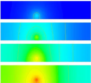
FIGURE1.6: Results of the Temperature Diffusion Problem for Time Steps 1, 16, 32 and 48 (top to bottom)

i+=1 t+=h

print("time step:",t)

mypde.setValue(Y=qH+rhocp/h*T) T=mypde.getSolution()

saveVTK("T.%d.vtu"%i, temp=T)

The script will create the filesT.1.vtu,T.2.vtu,. . .,T.50.vtuin the directory where the script has been started. The files contain the temperature distributions at time steps1,2, i, . . . ,50in theVTKfile format.

Figure1.6shows the result for some selected time steps. An easy way to visualize the results is the command mayavi2 -d T.1.vtu -m Surface

Use theConfigure Datawindow inMayavi2to move forward and backward in time.

1.4 Wave Propagation

In this next example we want to calculate the displacement fielduifor any timet >0by solving the wave equation:

ρui,tt−σij,j= 0 (1.31)

in a three dimensional block of lengthL inx0 andx1 direction and heightH inx2 direction. ρis the known

density which may be a function of its location. σij is the stress field which in case of an isotropic, linear elastic material is given by

σij=λuk,kδij+µ(ui,j+uj,i) (1.32)

whereλandµare the Lam´e coefficients andδijdenotes the Kronecker symbol. On the boundary the normal stress is given by

σijnj= 0 (1.33)

for all timet >0.

Here we are modelling a point source at the pointxCin thex0-direction which is a negative pulse of amplitude

U0followed by the same positive pulse. In mathematical terms we use

u0(xC, t) =U0 √ 2(t−t0) α e 1 2− (t−t0 )2 α2 _(1.34)

(24)

-1 -0.8 -0.6 -0.4 -0.2 0 0.2 0.4 0.6 0.8 1 0 1 2 3 4 5

FIGURE1.7: Input Displacement at Source Point (α= 0.7,t0 = 3,U0= 1).

for allt≥0whereαis the width of the pulse andt0is the time when the pulse changes from negative to positive.

In the simulations we will chooseα= 0.3andt0 = 2(see Figure1.7) and apply the source as a constraint in a

sphere of small radius around the pointxC.

We use an explicit time integration scheme to calculate the displacement fielduat certain time markst(n), wheret(n) =t(n−1)+hwith time step sizeh >0. In the following the upper index(n)refers to values at time t(n). We use the Verlet scheme with constant time step sizehwhich is defined by

u(n)= 2u(n−1)−u(n−2)+h2a(n) (1.35) (1.36) for alln= 2,3, . . .. It is designed to solve a system of equations of the form

u,tt=G(u) (1.37)

where one setsa(n)₌_G(u(n−1)₎_.

In our casea(n)_{is given by}

ρa(_in)=σ(_ij,jn−1) (1.38) and boundary conditions

σ(_ijn−1)nj = 0 (1.39)

derived from Equation (1.33) where

σ(_ijn−1) = λu(_k,kn−1)δij+µ(u(_i,jn−1)+u(_j,in−1)). (1.40) We also need to apply the constraint

a(₀n)(xC, t) =U0 p (2.) α2 (4 (t−t0)3 α3 −6 t−t0 α )e 1 2− (t−t0 )2 α2 _(1.41) 24 1.4. Wave Propagation

(25)

-10 -8 -6 -4 -2 0 2 4 6 8 10 0 1 2 3 4 5

FIGURE1.8: Input Acceleration at Source Point (α= 0.7,t0= 3,U0= 1).

which is derived from equation1.34by calculating the second order time derivative (see Figure1.8). Now we have converted our problem for displacement,u(n)_{, into a problem for acceleration,}_a(n)_{, which depends on the solution}

at the previous two time stepsu(n−1)_and_u(n−2)_.

In each time step we have to solve this problem to get the accelerationa(n), and we will use theLinearPDE class of theesys.escript.linearPDEspackage to do so. The general form of the PDE defined through the LinearPDEclass is discussed in Section4.1. The form which is relevant here is

Dija

(n)

j =−Xij,j. (1.42)

The natural boundary condition

njXij = 0 (1.43)

is used. Withu=a(n)we can identify the values to be assigned toDandX:

Dij =ρδij Xij =−σ(_ijn−1) (1.44) Moreover we need to define the locationrwhere the constraint1.41is applied. We will apply the constraint on a small sphere of radiusRaroundxC(we will use 3% of the width of the domain):

qi(x) =

1 wherekx−xck ≤R

0 otherwise. (1.45)

The following script defines the functionwavePropagationwhich implements the Verlet scheme to solve our wave propagation problem. The argument domainwhich is aDomainclass object defines the domain of the problem. handtendare the time step size and the end time of the simulation. lam,muandrhoare material properties.

def wavePropagation(domain,h,tend,lam,mu,rho, x_c, src_radius, U0):

# lists to collect displacement at point source which is returned # to the caller

ts, u_pc0, u_pc1, u_pc2 = [], [], [], []

(26)

x=domain.getX()

# ... open new PDE ...

mypde=LinearPDE(domain)

mypde.getSolverOptions().setSolverMethod(SolverOptions.HRZ_LUMPING) kronecker=identity(mypde.getDim())

dunit=numpy.array([1., 0., 0.]) # defines direction of point source

mypde.setValue(D=kronecker*rho, q=whereNegative(length(x-xc)-src_radius)*dunit)

# ... set initial values ....

n=0

# for first two time steps

u=Vector(0., Solution(domain)) u_last=Vector(0., Solution(domain)) t=0

# define the location of the point source

L=Locator(domain, xc)

# find potential at point source

u_pc=L.getValue(u)

print("u at point charge=",u_pc) ts.append(t) u_pc0.append(u_pc[0]) u_pc1.append(u_pc[1]) u_pc2.append(u_pc[2]) while t<tend: t+=h

# ... get current stress ....

g=grad(u)

stress=lam*trace(g)*kronecker+mu*(g+transpose(g))

# ... get new acceleration ....

amplitude=U0*(4*(t-t0)**3/alpha**3-6*(t-t0)/alpha)*sqrt(2.)/alpha**2 \ *exp(1./2.-(t-t0)**2/alpha**2) mypde.setValue(X=-stress, r=dunit*amplitude)

a=mypde.getSolution()

# ... get new displacement ...

u_new=2*u-u_last+h**2*a

# ... shift displacements ....

u_last=u u=u_new n+=1

print(n,"-th time step, t=",t) u_pc=L.getValue(u)

print("u at point charge=",u_pc)

# save displacements at point source to file for t > 0

ts.append(t)

u_pc0.append(u_pc[0]) u_pc1.append(u_pc[1]) u_pc2.append(u_pc[2])

# ... save current acceleration in units of gravity and displacements if n==1 or n%10==0:

saveVTK("./data/usoln.%i.vtu"%(n/10), \ acceleration = length(a)/9.81, \ displacement = length(u), \

tensor = stress, Ux = u[0])

return ts, u_pc0, u_pc1, u_pc2

Notice that all coefficients of the PDE which are independent of timetare set outside thewhileloop. This is for efficiency reasons since it allows theLinearPDEclass to reuse information as much as possible when iterating over time.

The statement

(27)

mypde.getSolverOptions().setSolverMethod(SolverOptions.HRZ_LUMPING)

enables the use of an aggressive approximation of the PDE operator as a diagonal matrix formed from the co-efficient D. The approximation allows, at the cost of additional error, very fast solution of the PDE, see also Section4.4.

There are a few newesys.escriptfunctions in this example: grad(u)returns the gradient ui,j of u (in factgrad(g)[i,j]== ui,j). There are restrictions on the argument of thegradfunction, for instance the statementgrad(grad(u))will raise an exception. trace(g)returns the sum of the main diagonal ele-mentsg[k,k]ofgandtranspose(g)returns the matrix transpose ofg(i.e. transpose(g)[i,j]== g[j,i]).

We initialize the values of uand u_last to be zero. It is important to initialize both with the solution FunctionSpaceas they have to be seen as solutions of PDEs from previous time steps. In fact, thegraddoes not accept arguments with a certainFunctionSpace, for more details see Section3.2.3.

TheLocatorclass is designed to extract values at a given location (in this casexC) from functions such as the displacement vectoru. TypicallyLocatoris used in the following way:

L=Locator(domain, xc) u=...

u_pc=L.getValue(u)

The return valueu_pcis the value ofuat the locationxc8. The values are collected in the listsu_pc0,u_pc1 andu_pc2together with the corresponding time marker ints. These values are handed back to the caller. Later we will show ways to access these data.

One of the big advantages of the Verlet scheme is the fact that the problem to be solved in each time step is very simple and does not involve any spatial derivatives (which is what allows us to use lumping in this simulation). The problem becomes so simple because we use the stress from the last time step rather than the stress which is actually present at the current time step. Schemes using this approach are called explicit time integration schemes. The backward Euler scheme we have used in Chapter1.3is an example of an implicit scheme. In this case one uses the actual status of each variable at a particular time rather than values from previous time steps. This will lead to a problem which is more expensive to solve, in particular for non-linear cases. Although explicit time integration schemes are cheap to finalize a single time step, they need significantly smaller time steps than implicit schemes and can suffer from stability problems. Therefore they require a very careful selection of the time step sizeh.

An easy, heuristic way of choosing an appropriate time step size is the Courant-Friedrichs-Lewy condition (CFL condition) which says that within a time step information should not travel further than a cell used in the discretization scheme. In the case of the wave equation the velocity of a (p-) wave is given as qλ+2_ρµ so one should choosehfrom

h= 1 5

r _ρ

λ+ 2µ∆x (1.46)

where∆xis the cell diameter. The factor1₅ is a safety factor considering the heuristics of the formula.

The following script uses thewavePropagation function to solve the wave equation for a point source located at the bottom face of a block. The width of the block in each direction on the bottom face is 10km (x0and

x1directions, i.e.l0andl1). The variablenegives the number of elements inx0andx1directions. The depth

of the block is aligned with the x2-direction. The depth (l2) of the block in thex2-direction is chosen so that

there are 10 elements, and the magnitude of the depth is chosen such that the elements become cubic. We chose 10 for the number of elements in thex2-direction so that the computation is faster.Brick(n0, n1, n2, l0, l1, l2)

is an esys.finleyfunction which creates a rectangular mesh with n0 ×n1×n2 elements over the brick

[0, l0]×[0, l1]×[0, l2].

from esys.finley import Brick

ne = 32 # number of cells in x_0 and x_1 directions

width = 10000. # length in x_0 and x_1 directions

lam = 3.462e9 mu = 3.462e9 rho = 1154. tend = 60

U0 = 1. # amplitude of point source

8_{In fact, it is the finite element node which is closest to the given position. The usage of}_Locator_{is MPI safe.}

(28)

FIGURE1.9: Selected time steps (n= 11,22,32,36) of a wave propagation over a 10km×10km×3.125km block from a point source initially at (5km, 5km, 0) with time step sizeh= 0.02083. Color represents the displacement. Here the view is oriented onto the bottom face.

# spherical source at middle of bottom face

xc=[width/2.,width/2.,0.]

# define small radius around point xc

src_radius = 0.03*width

print("src_radius =",src_radius)

mydomain=Brick(ne, ne, 10, l0=width, l1=width, l2=10.*width/32.) h=(1./5.)*inf(sqrt(rho/(lam+2*mu))*inf(domain.getSize())

print("time step size =",h) ts, u_pc0, u_pc1, u_pc2 = \

wavePropagation(mydomain, h, tend, lam, mu, rho, xc, src_radius, U0)

Thedomain.getSize()function returns the local element size∆x. Usinginfensures that the CFL condi-tion1.46 holds everywhere in the domain.

The script is available aswave.pyin the example directory . To visualize the results from the data directory: mayavi2 -d usoln.1.vtu -m Surface

You can rotate this figure by clicking on it with the mouse and moving it around. Again useConfigure Datato move backward and forward in time, and also to choose the results (acceleration, displacement orux) by using Select Scalar. Figure1.9shows the results for the displacement at various time steps.

It remains to show some possibilities to inspect the collected datau_pc0,u_pc1andu_pc2. One way is to write the data to a file and then use an external package such asgnuplot[39], LibreOffice Calc or Excel to read the data for further analysis. The following code shows one possible way to write the data to the file./data/U_ pc.csv:

u_pc_data=FileWriter('./data/U_pc.csv')

for i in range(len(ts)):

u_pc_data.write("%f %f %f %f\n"%(ts[i],u_pc0[i],u_pc1[i],u_pc2[i])) u_pc_data.close()

(29)

-1.5 -1 -0.5 0 0.5 1 1.5 0 2 4 6 8 10 U_x U_y U_z

FIGURE1.10: Amplitude at Point source from the Simulation

The fileU_pc.csvstores 4 columns of data:t, ux, uy, uzrespectively, whereux, uy, uzare thex0, x1, x2

com-ponents of the displacement vectoruat the point source. These can be plotted easily using any plotting package. Ingnuplot[39] the command:

plot 'U_pc.csv' u 1:2 title 'U_x' w l lw 2, 'U_pc.csv' u 1:3 title 'U_y' w l lw 2, 'U_pc.csv' u 1:4 title 'U_z' w l lw 2

will reproduce Figure1.10(As expected this is identical to the input signal shown in Figure1.7). It is pointed out that we are not using the standardpythonopento write to the fileU_pc.csvas it is not safe when running esys.escriptunder MPI, see Chapter2for more details.

Alternatively, one can implement plotting the results at run time rather than in a post-processing step. This avoids the generation of an intermediate data file. Inescriptthe preferred way of creating 2D plots of time depen-dent data ismatplotlib. The following script creates the plot and writes it into the fileu_pc.pngin the PNG image format:

import matplotlib.pyplot as plt

if getMPIRankWorld() == 0:

plt.title("Displacement at Point Source")

plt.plot(ts, u_pc0, '-', label="x_0", linewidth=1) plt.plot(ts, u_pc1, '-', label="x_1", linewidth=1) plt.plot(ts, u_pc2, '-', label="x_2", linewidth=1) plt.xlabel('time')

plt.ylabel('displacement') plt.legend()

plt.savefig('u_pc.png', format='png')

You can add plt.show() to create an interactive browser window. Notice that by checking the condition getMPIRankWorld()==0the plot is generated on one processor only (in this case the rank 0 processor) when run underMPI.

Both options for processing the point source data are included in the example filewave.py. There are other options available to process these data in particular through theSciPy[35] package, e.g. Fourier transformations. It

(30)

is beyond the scope of this user’s guide to document the usage ofSciPy[35] for time series analysis but it is highly recommended to look in relevant readily available documentation.

1.5 Elastic Deformation

In this section we want to examine the deformation of a linear elastic body caused by expansion through a heat distribution. We want a displacement fielduiwhich solves the momentum equation:

−σij,j = 0 (1.47)

where the stressσis given by

σij =λuk,kδij+µ(ui,j+uj,i)−(λ+2

3µ)α(T−Tref)δij. (1.48) In this formulaλandµare the Lam´e coefficients,αis the temperature expansion coefficient,T is the temperature distribution andTref a reference temperature. Note that Equation (1.47) is similar to Equation (1.31) introduced in Section 1.4but the inertia termρui,tt has been dropped as we assume a static scenario here. Moreover, in comparison to the Equation (1.32) definition of stressσin Equation (1.48) an extra term is introduced to bring in stress due to volume changes through temperature dependent expansion.

Our domain is the unit cube

Ω ={(xi)|0≤xi≤1} (1.49)

On the boundary the normal stress component is set to zero

σijnj= 0 (1.50)

and on the face withxi= 0we set thei-th component of the displacement to0:

ui(x) = 0 where xi= 0 (1.51) For the temperature distribution we use

T(x) =T0e−βkx−x

c_k

(1.52) with a given positive constantβand locationxc_{in the domain.}

When we insert Equation (1.48) we get a second order system of linear PDEs for the displacementsuwhich is called the Lam´e equation. We want to solve this using theLinearPDEclass. For a system of PDEs and a solution with several components theLinearPDEclass takes PDEs of the form

−(Aijkluk,l),j =−Xij,j . (1.53) Ais a rank-4Dataobject andXis a rank-2Dataobject. We show here the coefficients relevant for the problem we are trying to solve. The full form is given in Equation (4.4). The natural boundary conditions take the form

njAijkluk,l=njXij (1.54)

while constraints take the form

ui=riwhereqi>0 (1.55)

randqare each a rank-1Dataobject. We can easily identify the coefficients in Equation (1.53):

Aijkl=λδijδkl+µ(δikδjl+δilδjk) (1.56)

Xij = (λ+2

3µ)α(T−Tref)δij (1.57)

(1.58) The characteristic functionqdefining the locations and components where constraints are set is given by:

qi(x) =

1 xi= 0

0 otherwise. (1.59)

(31)

Under the assumption thatλ,µ,βandTref are constant we may useYi = (λ+2₃µ)α Ti. However, this choice would lead to a different natural boundary condition which does not set the normal stress component as defined in Equation (1.48) to zero.

Analogous to the concept of symmetry for a single PDE, we call the PDE defined by Equation (1.53) symmetric if

Aijkl=Aklij (1.60)

(1.61) This Lam´e equation is in fact symmetric, given the difference inD anddas compared to the scalar case. The LinearPDEclass is notified of this fact by calling itssetSymmetryOnmethod.

After we have solved the Lam´e equation we want to analyse the actual stress distribution. Typically the von-Misesstress defined by

σmises= r 1 2((σ00−σ11) 2_{+ (σ} 11−σ22)2+ (σ22−σ00)2) + 3(σ201+σ 2 12+σ 2 20) (1.62)

is used to detect material damage. Here we want to calculate the von-Mises stress and write it to a file for visual-ization.

The following script, which is available inheatedblock.pyin the example directory, solves the Lam´e equation and writes the displacements and the von-Mises stress into a filedeform.vtuin theVTKfile format:

from esys.finley import Brick

lam=1. mu=0.1 alpha=1.e-6 xc=[0.3, 0.3, 1.] beta=8. T_ref=0. T_0=1. #... generate domain ... mydomain = Brick(l0=1., l1=1., l2=1., n0=10, n1=10, n2=10) x=mydomain.getX() #... set temperature ... T=T_0*exp(-beta*length(x-xc))

#... open symmetric PDE ...

mypde=LinearPDE(mydomain) mypde.setSymmetryOn()

#... set coefficients ...

C=Tensor4(0., Function(mydomain))

for i in range(mydomain.getDim()):

for j in range(mydomain.getDim()): C[i,i,j,j]+=lam C[i,j,i,j]+=mu C[i,j,j,i]+=mu msk=whereZero(x[0])*[1.,0.,0.] \ +whereZero(x[1])*[0.,1.,0.] \ +whereZero(x[2])*[0.,0.,1.] sigma0=(lam+2./3.*mu)*alpha*(T-T_ref)*kronecker(mydomain) mypde.setValue(A=C, X=sigma0, q=msk) #... solve pde ... u=mypde.getSolution()

#... calculate von-Mises stress

g=grad(u)

sigma=mu*(g+transpose(g))+lam*trace(g)*kronecker(mydomain)-sigma0

sigma_mises=sqrt(((sigma[0,0]-sigma[1,1])**2+(sigma[1,1]-sigma[2,2])**2+ \ (sigma[2,2]-sigma[0,0])**2)/2. \

(32)

FIGURE1.11: von-Mises Stress and Displacement Vectors

+3*(sigma[0,1]**2 + sigma[1,2]**2 + sigma[2,0]**2))

#... output ...

saveVTK("deform.vtu", disp=u, stress=sigma_mises)

Finally, the results can be visualized by calling

mayavi2 -d deform.vtu -f CellToPointData -m Vectors -m Surface

Note that the filter CellToPointData is applied to create a smoother representation of the von-Mises stress. Fig-ure1.11shows the results where the colour of the vertical planes represent the von-Mises stress and a horizontal plane of arrows shows the displacements vectors.

1.6 Stokes Flow

In this section we will look at Computational Fluid Dynamics (CFD) to simulate the flow of fluid under the influence of gravity. TheStokesProblemCartesianclass will be used to calculate the velocity and pressure of the fluid. The fluid dynamics is governed by the Stokes equation. In geophysical problems the velocity of fluids is low; that is, the inertial forces are small compared with the viscous forces, therefore the inertial terms in the Navier-Stokes equations can be ignored. For a body forcef, the governing equations are given by:

∇ ·(η(∇~v+∇T_~_v))_{− ∇p}₌_−f, _(1.63) with the incompressibility condition

∇ ·~v= 0. (1.64)

wherep,ηandf are the pressure, viscosity and body forces, respectively. Alternatively, the Stokes equations can be represented in Einstein summation tensor notation (compact notation):

−(η(vi,j+vj,i)),j−p,i=fi, (1.65) with the incompressibility condition

−vi,i= 0. (1.66)

The subscript commaidenotes the derivative of the function with respect toxi. The body forcefin Equation (1.65) is the gravity acting in thex3direction and is given asf =−gρδi3. The Stokes equation is a saddle point problem,

and can be solved using a Uzawa scheme. A class calledStokesProblemCartesianinesys.escript

(33)

can be used to solve for velocity and pressure. A more detailed discussion of the class can be found in Chapter 6. In order to keep numerical stability and satisfy the Courant-Friedrichs-Lewy condition (CFL condition), the time-step size needs to be kept below a certain value. The Courant number is defined as:

C=vδt

h (1.67)

whereδt,v, andhare the time-step, velocity, and the width of an element in the mesh, respectively. The velocity vmay be chosen as the maximum velocity in the domain. In this problem the time-step size was calculated for a Courant number of0.4.

The followingpythonscript is the setup for the Stokes flow simulation, and is available in the example directory asfluid.py. It starts off by importing the classes, such as theStokesProblemCartesianclass, for solving the Stokes equation and the incompressibility condition for velocity and pressure. Physical constants are defined for the viscosity and density of the fluid, along with the acceleration due to gravity. Solver settings are set for the maximum iterations and tolerance; the default solver used is PCG (Preconditioned Conjugate Gradients). The mesh is defined as a rectangle to represent the body of fluid. We are using20×20elements with piecewise linear elements for the pressure and for velocity but the elements are subdivided for the velocity. This approach is called macro elementsand needs to be applied to make sure that the discretized problem has a unique solution, see [13] for details9. The fact that pressure and velocity are represented in different ways is expressed by

velocity=Vector(0., Solution(mesh))

pressure=Scalar(0., ReducedSolution(mesh))

The gravitational force is calculated based on the fluid density and the acceleration due to gravity. The boundary conditions are set for a slip condition at the base and the left face of the domain. At the base fluid movement in the x0-direction is free, but fixed in thex1-direction, and similarly at the left face fluid movement in thex1-direction

is free but fixed in thex0-direction. An instance of theStokesProblemCartesianclass is defined for the

given computational mesh, and the solver tolerance set. Inside thewhileloop, the boundary conditions, viscosity and body force are initialized. The Stokes equation is then solved for velocity and pressure. The time-step size is calculated based on the Courant-Friedrichs-Lewy condition (CFL condition), to ensure stable solutions. The nodes in the mesh are then displaced based on the current velocity and time-step size, to move the body of fluid. The output for the simulation of velocity and pressure is then saved to a file for visualization.

from esys.escript import *

import esys.finley

from esys.escript.models import StokesProblemCartesian

# physical constants eta=1. rho=100. g=10. # solver settings tolerance=1.0e-4 max_iter=200 t_end=50 t=0.0 time=0 verbose=True # define mesh H=2. L=1. W=1.

mesh = esys.finley.Rectangle(l0=L, l1=H, order=-1, n0=20, n1=20) coordinates = mesh.getX()

9_{Alternatively, one can use second order elements for the velocity and first order elements for pressure on the same element. You can set} order=2inesys.finley.Rectangle.

(34)

# gravitational force

Y=Vector(0., Function(mesh)) Y[1] = -rho*g

# element spacing

h = Lsup(mesh.getSize())

# boundary conditions for slip at base

boundary_cond=whereZero(coordinates[1])*[0.0,1.0]+whereZero(coordinates[0])*[1.0,0.0]

# velocity and pressure vectors

velocity=Vector(0., Solution(mesh)) pressure=Scalar(0., ReducedSolution(mesh)) # Stokes Cartesian solution=StokesProblemCartesian(mesh) solution.setTolerance(tolerance) while t <= t_end:

print(" --- Time step = %s ---"%t)

print("Time = %s seconds"%time)

solution.initialize(fixed_u_mask=boundary_cond, eta=eta, f=Y)

velocity,pressure=solution.solve(velocity,pressure,max_iter=max_iter, \ verbose=verbose)

print("Max velocity =", Lsup(velocity), "m/s")

# CFL condition

dt=0.4*h/(Lsup(velocity))

print("dt =", dt)

# displace the mesh

displacement = velocity * dt coordinates = mesh.getX()

newx=interpolate(coordinates + displacement, ContinuousFunction(mesh)) mesh.setX(newx)

time += dt

vel_mag = length(velocity)

#save velocity and pressure output

saveVTK("vel.%2.2i.vtu"%t, vel=vel_mag, vec=velocity, pressure=pressure) t = t+1.

The results from the simulation can be viewed withMayavi2, by executing the following command:

mayavi2 -d vel.00.vtu -m Surface

Colour-coded scalar maps and velocity flow fields can be viewed by selecting them in the menu. The time-steps can be swept through to view a movie of the simulation. Figure1.12shows the simulation output. Velocity vectors and a colour map for pressure are shown. As the time progresses the body of fluid falls under the influence of gravity. The view used here to track the fluid is the Lagrangian view, since the mesh moves with the fluid. One of the disadvantages of using the Lagrangian view is that the elements in the mesh become severely distorted after a period of time and introduce solver errors. To get around this limitation the Level Set Method can be used, with the Eulerian point of view for a fixed mesh.

(35)

(a) t=1 (b) t=20 (c) t=30

(d) t=40 (e) t=50 (f) t=60

FIGURE1.12: Simulation output for Stokes flow. Fluid body starts off as a rectangular shape, then progresses downwards under the influence of gravity. Colour coded distribution represents the scalar values for pressure. Velocity vectors are displayed at each node in the mesh to show the flow field. Computational mesh used was 20×20 elements.

1.7 Slip on a Fault

In this example we illustrate how to calculate the stress distribution around a fault in the Earth’s crust caused by a slip through an earthquake.

To simplify the presentation we assume a simple domainΩ = [0,1]2 with a vertical fault in its center as illustrated in Figure1.13. We assume that the slip distributionsion the fault is known. We want to calculate the distribution of the displacementsuiand stressσij in the domain. Further, we assume an isotropic, linear elastic material model of the form

σij = λuk,kδij+µ(ui,j+uj,i) (1.68)

whereλandµare the Lam´e coefficients andδijdenotes the Kronecker symbol. On the boundary the normal stress is given by

σijnj= 0 (1.69)

and normal displacements are set to zero:

uini= 0 (1.70)

The stress needs to fulfill the momentum equation

−σij,j = 0 (1.71)

This problem is very similar to the elastic deformation problem presented in Section 1.5. However, we need to address an additional challenge: the displacementui is in fact discontinuous across the fault, but we are in the

(36)

Fault (0.5, 0.75) (0.5, 0.25) (1, 1) (0, 0) FIGURE1.13: DomainΩ = [0,1]2

with a vertical fault of length0.5.

lucky situation that we know the jump of the displacements across the fault. This is in fact the given slipsi. So we can split the total distributionuiinto a componentviwhich is continuous across the fault and the known slipsi

ui=vi+ 1 2s

±

i (1.72)

wheres±=swhen right of the fault ands±=−swhen left of the fault. We assume thats±= 0when sufficiently away from the fault.

We insert this into the stress definition in Equation (1.68) σij = σcij+ 1 2σ s ij (1.73) with σc_ij=λvk,kδij+µ(vi,j+vj,i) (1.74) and σs_ij =λs±_k,kδij+µ(s±i,j+s ± j,i). (1.75) In fact, σs

ij defines a stress jump across the fault. An easy way to construct this function is to use a functionχ which is1on the right and−1on the left side from the fault. One can then set

σ_ijs =χ·(λsk,kδij+µ(si,j+sj,i)) (1.76) assuming thatsis extended by zero away from the fault. After inserting Equation (1.73) into (1.71) we get the differential equation −σcij,j= 1 2σ s ij,j (1.77)

Together with the definition (1.74) we have a differential equation for the continuous functionvi. Notice that the boundary condition (1.70) and (1.69) transfer toviandσijc assis zero away from the fault. In Section1.5we have discussed how this problem is solved using theLinearPDEclass. We refer to this section for further details.

To define the fault we use theFaultSystemclass introduced in Section6.4. The following statements define a fault systemfsand add the fault1to the system:

(37)

fs=FaultSystem(dim=2)

fs.addFault(fs.addFault(V0=[0.5,0.25], strikes=90*DEG, ls=0.5, tag=1)

The fault added starts at point(0.5,0.25)has length0.5and points north. The main purpose of theFaultSystem class is to define a parameterization of the fault using a local coordinate system. One can inquire the class to get the range used to parameterize a fault.

p0,p1 = fs.getW0Range(tag=1)

Typically p0is equal to zero whilep1 is equal to the length of the fault. The parameterization is given as a mapping from a set of local coordinates onto a parameter range (in our case the rangep0top1). For instance, to map the entire domainmydomainonto the fault one can use

x = mydomain.getX()

p,m = fs.getParametrization(x, tag=1)

Of course there is the problem that not all locations are on the fault. For those locations which are on the faultmis set to 1, otherwise 0 is used. So on return the values ofpdefine the value of the fault parameterization (typically the distance from the starting point of the fault along the fault) wheremis positive. On all other locations the value ofpis undefined. Nowpcan be used to define a slip distribution on the fault via

s = m*(p-p0)*(p1-p)/((p1-p0)/2)**2*slip_max*[0.,1.]

Notice the factormwhich ensures thatsis zero away from the fault. It is important that the slip is zero at the ends of the faults.

We can now put all components together to get the script: from esys.escript import _*

from esys.escript.models import FaultSystem

from esys.escript.unitsSI import DEG

lam=1. mu=1

slip_max=1.

mydomain = Rectangle(l0=1.,l1=1.,n0=16, n1=16) # n1 needs to be a multiple of 4! # .. create the fault system

fs=FaultSystem(dim=2)

fs.addFault(V0=[0.5,0.25], strikes=90*DEG, ls=0.5, tag=1)

# ... create a slip distribution on the fault

p, m=fs.getParametrization(mydomain.getX(), tag=1) p0,p1= fs.getW0Range(tag=1)

s=m*(p-p0)*(p1-p)/((p1-p0)/2)**2*slip_max*[0.,1.]

# ... calculate stress according to slip:

D=symmetric(grad(s))

chi, d=fs.getSideAndDistance(D.getFunctionSpace().getX(), tag=1) sigma_s=(mu*D+lam*trace(D)*kronecker(mydomain))*chi

#... open symmetric PDE ...

mypde=LinearPDE(mydomain) mypde.setSymmetryOn()

#... set coefficients ...

C=Tensor4(0., Function(mydomain))

for i in range(mydomain.getDim()):

for j in range(mydomain.getDim()): C[i,i,j,j]+=lam

C[j,i,j,i]+=mu C[j,i,i,j]+=mu

# ... fix displacement in normal direction

x=mydomain.getX()

msk=whereZero(x[0])*[1.,0.] + whereZero(x[0]-1.)*[1.,0.] \ +whereZero(x[1])*[0.,1.] + whereZero(x[1]-1.)*[0.,1.]

esys-Escript User’s Guide: Solving Partial Differential Equations with Escript and Finley Release - 4.1 (r5754)

esys-Escript

User’s Guide:

Solving Partial Differential Equations

with Escript and Finley

Release - 4.1

(r5754)

Lutz Gross

et al.

(Editor)

24 July 2015

Centre for Geoscience Computing (GeoComp)

School of Earth Sciences

The University of Queensland

Brisbane, Australia

Guide to Documentation

Researchers and Developers

Contents

CHAPTER

ONE

Tutorial: Solving PDEs

1.1

Installation

1.2

The First Steps

1.2.1

Plotting Using

matplotlib

1.2.2

Visualization using export files

x

x

n

T

1.3

The Diffusion Problem

1.3.1

Outline

1.3.2

Temperature Diffusion

1.3.3

Helmholtz Problem

1.3.4

The Transition Problem

1.4

Wave Propagation

1.5

Elastic Deformation

1.6

Stokes Flow

1.7

Slip on a Fault