High-Performance Computing: Do’s and Dont’s

3,300+

OPEN ACCESS BOOKS

107,000+

INTERNATIONAL

AUTHORS AND EDITORS

113+ MILLION

BOOKS

DELIVERED TO 151 COUNTRIES

AUTHORS AMONG

TOP 1%

MOST CITED SCIENTIST

12.2%

AUTHORS AND EDITORS FROM TOP 500 UNIVERSITIES

Selection of our books indexed in the Book Citation Index in Web of Science™ Core Collection (BKCI)

Chapter from the book Computational Fluid Dynamics - Basic Instruments and Applications in Science

Downloaded from: http://www.intechopen.com/books/computational-fluid-dynamics-basic-instruments-and-applications-in-science

World's largest Science,

Technology & Medicine

Open Access book publisher

Interested in publishing with InTechOpen?

Chapter 1

High-Performance Computing: Dos and Don’ts

Guillaume Houzeaux, Ricard Borrell, Yvan Fournier,

Marta Garcia-Gasulla, Jens Henrik Göbbert,

Elie Hachem, Vishal Mehta, Youssef Mesri,

Herbert Owen and Mariano Vázquez

http://dx.doi.org/10.5772/intechopen.72042

Provisional chapter

High-Performance Computing: Dos and Don

’

ts

Guillaume Houzeaux, Ricard Borrell,

Yvan Fournier, Marta Garcia-Gasulla,

Jens Henrik Göbbert, Elie Hachem,

Vishal Mehta, Youssef Mesri, Herbert Owen

and Mariano Vázquez

Additional information is available at the end of the chapter

Abstract

Computational fluid dynamics (CFD) is the main field of computational mechanics that has historically benefited from advances in high-performance computing. High-performance computing involves several techniques to make a simulation efficient and fast, such as distributed memory parallelism, shared memory parallelism, vectorization, memory access optimizations, etc. As an introduction, we present the anatomy of super-computers, with special emphasis on HPC aspects relevant to CFD. Then, we develop some of the HPC concepts and numerical techniques applied to the complete CFD simu-lation framework: from preprocess (meshing) to postprocess (visualization) through the simulation itself (assembly and iterative solvers).

Keywords:parallelization, high-performance computing, assembly, supercomputing,

meshing, adaptivity, algebraic solvers, parallel I/O, visualization

1. Introduction to high-performance computing

1.1. Anatomy of a supercomputer

Computational fluid dynamics (CFD) simulations aim at solving more complex, more real, more detailed, and bigger problems. To achieve this, they must rely on high-performance computing (HPC) systems as it is the only environment where these kinds of simulations can be performed [1].

At the same time, HPC systems are becoming more and more complex and the hardware is exposing massive parallelism at all levels, making a challenge exploiting the resources.

© The Author(s). Licensee InTech. This chapter is distributed under the terms of the Creative Commons Attribution License (http://creativecommons.org/licenses/by/3.0), which permits unrestricted use, distribution, and eproduction in any medium, provided the original work is properly cited.

© 2018 The Author(s). Licensee InTech. This chapter is distributed under the terms of the Creative Commons Attribution License (http://creativecommons.org/licenses/by/3.0), which permits unrestricted use, distribution, and reproduction in any medium, provided the original work is properly cited.

In order to understand the concepts that are explained in the following sections, we explain briefly the different levels of parallelism available in a supercomputer. We do not aim at giving a full description or state of the art of the different architectures available in supercomputers, but a general overview of the most common approaches and concepts. First, we depict the different levels of hardware that form a supercomputer.

1.1.1. Hardware

Core/Central Processing Unit:We could consider a core as the first unit of computation, and a core is able to decode instructions and execute them. Here, within the core, we find the first and most low level of parallelism: the instruction-level parallelism. This kind of parallelism is offered by superscalar processors, and its main characteristic is that they can execute more than one instruction during a clock cycle. There are several developments that allow instruction-level parallelism such as pipelining, out-of-order execution, or multiple execution units. These tech-niques are the ones that allow to obtain instructions per cycle (IPC) higher than one. The exploitation of this parallelism relies mainly on the compiler and on the hardware units itself. Reordering of instructions, branch prediction, renaming or memory access optimization are some of the techniques that help to achieve a high level of instruction parallelism.

At this level, complementary to instruction-level parallelism, we can find data-level parallel-ism offered by vectorization. Vectorization allows to apply the same operation to multiple pieces of data in the context of a single instruction. The performance obtained by this kind of processors depends highly on the type of code that it is executing. Scientific applications or numerical simulations are often codes that can benefit from this kind of processors as the kind of computation they must perform usually consists in applying the same operation to large pieces of independent data. We briefly see how this technique can accelerate the assembly process in Section 4.4.

Socket/Chip:Coupling of several cores in the same integrated circuit is a common approach and is usually referred as multicore or many-core processors (depending on the amount of cores it aggregates, one name or the other is used). One of the main advantages is that the different cores share some levels of cache. The shared caches can improve the reuse of data by different threads running on cores in the same socket, with the added advantage of the cores being close on the same die (higher clock rates, less signal degradation, less power).

Having several cores in the same socket allows to have thread-level parallelism, as each different core can run a different sequence of instructions in parallel but having access to the same data. Section 4.2 studies this parallelism through the use of OpenMP programming interface.

Accelerators/GPUs:Accelerators are a specialized hardware that includes hundreds of com-puting units that can work in parallel to solve specific calculations over wide pieces of data. They include its own memory. Accelerators need a central processing unit (CPU) to process the main code and off-load the specific kernels to them. To exploit the massive parallelism avail-able within the GPUs, the application kernels must be rewritten. The dominant programming language is OpenCL that is cross-platform, while other alternatives are vendor dependent (e.g., CUDA [2]).

Node:A computational node can include one or several sockets and accelerators along with main memory and I/O. A computational node is, therefore, the minimum autonomous com-putation unit as it includes cores to compute, memory to store data, and network interface to communicate. The main classification of shared memory nodes is based on the kind of mem-ory access they have: uniform memmem-ory access (UMA) or [3] nonuniform memmem-ory access (NUMA). In UMA systems, the memory system is common to all the processors and this means that there is just one memory controller that can only serve one petition at the same time; when having several cores issuing memory requests, this becomes a bottleneck. On the other hand, NUMA nodes partition the memory among the different processors; although the main memory is seen as a whole, the access time depends on the memory location relative to the processor issuing the request.

Within the node, also thread-level parallelism can be exploited as the memory is shared among the different cores inside the node.

Cluster/Supercomputer: A supercomputer is an aggregation of nodes connected through a high-speed network with a specialized topology. We can find different network topologies (i.e., how the nodes are connected), such as 2D or 3D Torus or Hypercube. The kind of network topology will determine the number of hoops that a message will need to reach its destination or communication bottlenecks. A supercomputer usually includes a distributed file system to offer a unified view of the cluster from the user point of view.

The parallelism that can be used at the supercomputer level is a distributed memory approach. In this case, different processes can run in different nodes of the cluster and communicate through the interconnect network when necessary. We go through the main techniques of such parallelism applied to the assembly and iterative solvers in Sections 4.1 and 5.2, respectively.

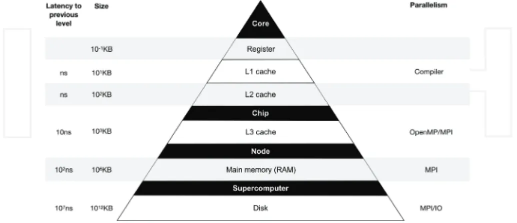
Figure 1shows the different levels of hardware of a supercomputer presented previously, together with the associated memory latency and size, as well as the type of parallelism to

Figure 1.Anatomy of a supercomputer. Memory latency and size (left) and parallelism (right) to exploit the different levels of hardware (middle).

exploit them. The numbers are expressed in terms of orders of magnitude and pretend to be only orientative as they are system dependent.

We have seen all the computational elements that form a supercomputer from a hierarchical point of view. All these levels that have been explained also include different levels of storage that are organized in a hierarchy too. Starting from the core, we can find the registers where the operands of the instructions that will be executed are stored. Usually included also in the core or CPU, we can find the first level of cache and this is the smallest and fastest one; it is common that it is divided in two parts: one to store instructions (L1i) and another one to store data (L1d). The second level of cache (L2) is bigger, still fast, and placed close to the core too. A common configuration is that the third level of cache (L3) is shared at the socket and L1 and L2 private to the core, but any combination is possible.

The main memory can be of several gigabytes (GB) and much slower than the caches. It is shared among the different processors of the node, but as we have explained before it can have a nonuniform memory access (NUMA), meaning that it is divided in pieces among the differ-ent sockets. At the supercomputer level, we find the disk that can store petabytes of data.

1.1.2. Software

We have seen an overview of the hardware available within a supercomputer and the different levels of parallelism that it exposes. The different levels of the HPC software stack are designed to help applications exploit the resources of a supercomputer (i.e., operating system, compiler, runtime libraries, and job scheduler). We focus on the parallel programming models because they are close to the application and specifically on OpenMP and MPI because they are the standard“de facto”at the moment in HPC environments.

OpenMP: It is a parallel programming model that supports C, C++, and Fortran [4]. It is based on compiler directives that are added to the code to enable shared memory parallel-ism. These directives are translated by the compiler supporting OpenMP into calls to the corresponding parallel runtime library. OpenMP is based on a fork-join model, meaning that just one thread will be executing the code until it reaches a parallel region; at this point, the additional threads will be created (fork) to compute in parallel and at the end of the parallel region all the threads willjoin. The communication in OpenMP is done implicit through the shared memory between the different threads, and the user must annotate for the different variables the kind of data sharing they need (i.e., private, shared). OpenMP is a standard defined by a nonprofit organization: OpenMP Architecture Review Board (ARB). Based on this definition, different commercial or open source compilers and runtime libraries offer their own implementation of the standard.

The loop parallelism in OpenMP had been the most popular in scientific applications. The main reason is that it fits perfectly the kind of code structure in these applications: loops. And this allows a very easy and straightforward parallelization of the majority of codes.

Since OpenMP 4.0, the standard also includes task parallelism which together with depen-dences offers a more flexible and powerful way of expressing parallelism. But these advan-tages have a cost: the ease of programming. Scientific programmers still have difficulties in

expressing parallelism with tasks because they are used at seeing the code as a single flow with some parallel regions in it.

In Section 4.2, we describe how loop and task parallelism can be applied to the algebraic system assembly.

MPI:The message passing interface (MPI) is a parallel programming model based on an API for explicit communication [5]. It can be used in distributed memory systems and shared memory environments. The standard is defined by the MPI Forum, and different implementations of this standard can be found. In the execution model of MPI, all the processes will run themain()

function in parallel. In general, MPI follows a single program multiple data (SPMD) approach although it allows to run different binaries under the same MPI environment (multicode cou-pling [6]).

1.2. HPC concepts

The principal metrics used in HPC are the second (sec) for time measurements, the floating point operation (flop) for counting arithmetic operations, and the binary term (byte) to quantify memory. A broad range of unit prefixes are required; for example, the time spent on individual operations is generally expressed in terms of nanoseconds (ns), the computing power of a high-end supercomputer is expressed in terms of petaflops (1015flop/sec), and the main memory of a computing node is quantified in terms of gigabytes (GB). There are also more specific metrics, for example,cache missesare used to count the data fetched from the main memory to the cache, and the IPC index refers to the instructions per clock cycle carried out by a CPU.

The principal measurements used to quantify the parallel performance are the load balance, the strong speedup, and the weak speedup. The load balance measures the quality of the workload distribution among the computing resources engaged for a computational task. If

timeidenotes the time spent by processi, out ofnpprocesses, on the execution of such parallel

task, the load balance can be expressed as the average time, aveiðtimeiÞ, divided by the

maxi-mum time, maxiðtimeiÞ. This value represents also the ratio between the resources effectively

used with respect to the resources engaged to carry out the task. In other words, the load balance ∈½0;1is equivalent to the efficiency achieved on the usage of the resources:

efficiency≔

P

itime ncoremaxiðtimeiÞ¼

aveiðtimeiÞ

maxiðtimeiÞ≕

load balance:

Another common measurement is the strong speedup that measures the relative acceleration achieved at increasing the computing resources used to execute a specific task. IfT pð Þis the time achieved to carry out the task under consideration usingpparallel processes, the strong speedup achieved at increasing the number of processes fromp₁top₂p₁<p₂is

strong speedup≔ T p1

T Pð Þ2

,

parallel efficiency≔ T p1 p2

T p₂ p₁:

Finally, the weak speedup measures the relative variation on the computing time when the workload and the computing resources are increased proportionally. IfT nð ;pÞrepresents the time spent on the resolution of a problem of sizenwithpparallel processes, the weak speedup at increasing the number of parallel processes fromp₁top₂(and thus multiplying the problem size byp2 p₁) is defined as: weak speedup≔ T np1 p₂ p₂ T p₂ p₁ :

In the CFD context, the weak speedup is measured at increasing proportionally the mesh size and the computational resources engaged on the simulation. The ideal result for the speedup would be 1; however, this is hardly possible because the complexity of some parts of the problem, such as the solution of the linear system, increases above the linearity (see Section 5.4 on domain decomposition (DD) preconditioners). A second degradation factor is the communication costs, necessary to transfer data between parallel processes in a distributed memory context. This is especially relevant for the strong speedup tests: the overall workload is kept constant, and therefore, the workload per parallel process reduces at increasing the computing resources; consequently, while the computing time reduces, the overhead produced by the communications grows.

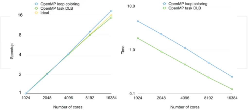
While the strong and weak speedups measure the relative performance of a piece of code by varying the number of processes, the load balance is a measure of the proper exploitation of a particular amount of resources. An unbalanced computation can be perfectly scalable if the dominant part is properly distributed on the successive partitions. This situation can be observed inFigure 9from Section 4. It shows the strong scalability and the timings for two different parallel methods for matrix assembly. The faster method is not the one that shows better strong scaling, and in this case, it is the one that guarantees a better load balance between the different parallel processes.

Nonetheless, a balanced and scalable code does not mean yet an optimal code in terms of performance. The aforementioned measurements account for the use of parallel resources but do not say anything about how fast the code is at performing a task. In particular, if we consider a sequential code to be parallelized, the more efficient it is, the harder it will be to achieve good scalability since the communication overheads will be more relevant. Indeed,

“the easiest way of making software scalable is to make it sequentially inefficient”[7].

CFD is considered a memory-bounded application, and this means that sequential performance is limited by the cost of fetching data from the main to the cache memory, rather than by the cost of performing the computations on the CPU registers. The reason is that the sparse operations, which dominate CFD computations, have a low arithmetic intensity (flops/byte), that is, few operations are performed for each byte moved from the main memory to the cache memory.

Therefore, the sequential performance of CFD codes is mostly determined by the management of the memory transfers. A strategy to reduce data transfers is to maximize the data locality. This means to maximize the reuse of the data uploaded to the cache by: (1) using the maximum percentage of the bytes contained in each block (referred ascache line) uploaded to the cache, known as spatial locality, or (2) reuse data that have been previously used and kept into the cache, known as temporal locality. An example illustrates data locality in Section 4.4.

1.2.1. Challenges

Moore’s law says:The number of transistors in a dense integrated circuit doubles approximately every two years. This law formulated in 1965 not only proved to be true, but it also translated in doubling the computing capacity of the cores every 24 months. This was possible not only by increasing the number of transistors but by increasing the frequency at which they worked. But, in the last years, it has come what computer scientists callThe End of Free Lunch. This refers to the fact that the performance of a single core is not being increased at the same pace. There are three main issues that explain this:

The memory wall: It refers to the gap in performance that exists between processor and memory [8] (CPU speed improved at an annual rate of 55% up to 2000, while memory speed only improved at 10%). The main method for bridging the gap has been to use caches between the processor and the main memory, increasing the sizes of these caches and adding more levels of caching. But memory bandwidth is still a problem that has not been solved.

The ILP wall:Increasing the number of transistors in a chip as Moore’s law says is used in some cases to increase the number of functional units, allowing a higher level of instruction-level parallelism (ILP) because there are more specialized units or several units of the same kind (i.e., two floating point units that can process two floating point operations in parallel). But finding enough parallelism in a single instruction stream to keep a high-performance single-core processor busy is becoming more and more complex. One of the techniques to overcome this has been hyper-threading. This consists in a single physical core to appear as two (or more) to the operating system. Running two threads will allow to exploit the instruction-level parallelism.

The power wall:As we said, not only the number of transistors was increasing but also the frequency was increasing. But there exists a technological limit to surface power density, and for this reason, clock frequency cannot scale up freely any more. Not only the amount of power that must be supplied would not be assumable, but the chip would not be able to dissipate the amount of heat generated. To address this issue, the trend is to develop more simple and specialized hardware and aggregate more of them (i.e., Xeon Phi, GPUs).

Nevertheless, computer scientists still want to achieve the Exascale machine, but they cannot rely on increasing the performance of a single core as they used to. The turnaround is that the number of cores per chip and per node is growing quite fast in the last years, along with the number of nodes in a cluster. This is pushing the research into more complex memory hierar-chies and networks topologies.

Once the Exascale machines are available, the challenge is to have applications that can make an efficient use and scale there. The increase in complexity of the hardware is a challenge for scientific application developers because their codes must be efficient in more complex hard-ware and address a high level of parallelism at both shared and distributed memory levels. Moreover, rewriting and restructuring existing codes is not always feasible; in some cases, the amount of lines of code is hundreds of thousands and, in others, the original authors of those codes are not around anymore.

At this point, only a unified effort and a codesign approach will enable Exascale applications. Scientists in charge of HPC applications need to trust in the parallel middleware and runtimes available to help them exploit the parallel resources. The complexity and variety of the hard-ware will not allow anymore the manual tuning of the codes for each different architecture.

1.3. Anatomy of a CFD simulation

A CFD simulation can be divided into four main phases: (1) mesh generation, (2) setup, (3) solution, and (4) analysis and visualization. Ideally, these phases would be carried out consec-utively, but, in practice, they are interleaved until a satisfactory solution is achieved. For example, on the solution analysis, the user may realize that the integration time was not enough or that the quality of the mesh was too poor to capture the physical phenomena being tackled. This would force to return to the solution or to the mesh generation phase, respec-tively. Indeed, supported by the continued increase of the computing resources available, CFD simulation frameworks have evolved toward a runtime adaptation of the numerical and computational strategies in accordance with the ongoing simulation results. This dynamicity includes mesh adaptivity, in situ analysis and visualization, and runtime strategies to optimize the parallel performance. These mechanisms make simulation frameworks more robust and efficient.

The following sections of this chapter outline the numerical methods and computational aspects related with the aforementioned phases. Section 2 is focused on meshing and adaptiv-ity, and Section 3 on the partitioning required for the parallelization. Sections 4 and 5 focus on the two main parts of the solution phase, that is, the assembly and the solution of the algebraic system. Finally, Section 6 is focused on the I/O and visualization issues.

2. Meshing and adaptivity

Mesh adaptation is one of the key technologies to reduce both the computational cost and the approximation errors of PDE-based numerical simulations. It consists in introducing local mod-ifications into the computational mesh in such a way that the calculation effort to reach a certain level of error is minimized. In other words, adaptation strategies maximize the accuracy of the obtained solution for a given computational budget. Three main components constitute the mesh adaptation process: error estimators to derive and make decisions where and when mesh adap-tation is required and remeshing mechanics to change the density and orienadap-tation of mesh entities. Last but not least, dynamic load balancing is to ensure efficient computations on parallel

systems. We develop the main ideas behind the first two concepts in the following subsections, and mesh partitioning and dynamic load balance are considered in Section 3.

2.1. Error estimators and adaptivity

The discretization of a continuous problem leads to an approximate solution more or less representative of the exact solution according to the care given to the numerical approximation and mesh resolution. Therefore, in order to be able to certify the quality of a given calculation, it is necessary to be able to estimate the discretization error—between this approximated solution, resulting for example from the application of the finite element (FE) or volume methods, and the exact (often unknown) solution of the continuous problem. This field of research has been the subject of much investigation since the mid-1970s. The first efforts focused on the a priori convergence properties of finite element methods to upper-bound the gap between the two solutions. Since a priori error estimate methods are often insufficient to ensure reliable estimation of the discretization error, new estimation methods called a posteriori are rather quickly pre-ferred. Once the approximate solution has been obtained, it is then necessary to study and quantify its deviation from the exact solution. The error estimators of this kind provide informa-tion overall the computainforma-tional domain, as well as a map of local contribuinforma-tions which is useful to obtain a solution satisfying a given precision by means of adaptive procedures. One of the most popular methods of this family is the error estimation based on averaging techniques, as those proposed in [9]. The popularity of these methods is mainly due to their versatile use in aniso-tropic mesh adaptation tools as a metric specifying the optimal mesh size and orientation with respect to the error estimation. An adapted mesh is then obtained by means of local mesh modificationsto fit the prescribed metric specifications. This approach can lead to elements with large angles that are not suitable for finite element computations as reported in the general standard error analysis for which some regularity assumption on the mesh and on the exact solution should be satisfied. However, if the mesh is adapted to the solution, it is possible to circumvent this condition [10].

We focus now on anisotropic mesh adaptation driven by directional error estimators. The latter are based on the recovery of the Hessian of the finite element solution. The purpose is to achieve an optimal mesh minimizing the directional error estimator for a constant number of mesh elements. It allows, as shown inFigure 2, to refine/coarsen the mesh, stretch and orient the elements in such a way that, along the adaptation process, the mesh becomes aligned with the fine scales of the solution whose locations are unknown a priori. As a result of this, highly accurate solutions are obtained with a much lower number of elements. More recently, estimation techniques have also been developed to evaluate the error commit-ted on quantities of interest (e.g., drag, lift, shear, and heat flux) to the engineer. On this point, the current trend is to develop upper and lower bounds to delimit the observed physical quantity [11].

2.2. Parallel meshing and remeshing

The parallelization of mesh adaptation methods goes back to the end of the 1990s. The SPMD MPI-based paradigm has been adopted by the pioneering works [12–14]. The effectiveness of

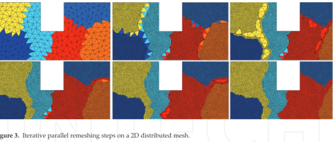
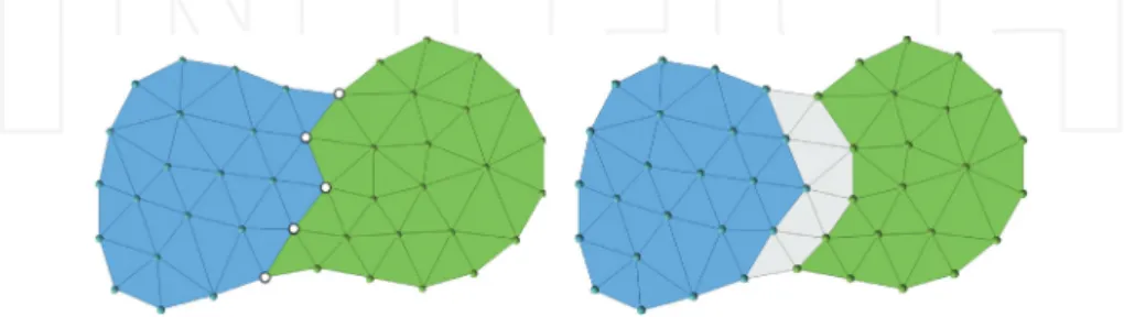
these methods depends on the repartitioning algorithms used and on how the interfaces between subdomains are managed. Indeed, mesh repartitioning is the key process for most of today’s parallel mesh adaptation methods [15]. Starting from a partitioned mesh into multiple subdomains, remeshing operations are performed using a sequential mesh adaptator on each subdomain with an extra treatment of the interfaces. Two main approaches are considered in the literature: (1) It is an iterative one. At the first iteration, remeshing is performed concurrently on each processor, while the interfaces between subdomains are locked to avoid any modification in the sequential remeshing kernel. Then, a new partitioning is calculated to move the interfaces and remesh them at the next iteration. The algorithm iterates until all items have been remeshed (Figure 3). (2) The second approach consists in handling the interfaces by considering a comple-mentary data structure to manage remeshing on remote mesh entities.

The first approach is preferred because of its high efficiency and full code-reusing capability for sequential remeshing kernels. However, hardware architectures go to be more dense (more cores per compute node) than before to fit the energy constraints fixed as asine qua none

condition to target Exascale supercomputers. Indeed, it is assumed that the nodes of a future Exascale system will contain thousands of cores per node. Therefore, it is important to rethink meshing algorithms in this new context of high levels of parallelism and using fine-grain parallel programming models that exploit the memory hierarchy. However, unstructured data-based applications are hard to parallelize effectively on shared-memory architectures for reasons described in [16].

It is clear that one of the main challenges to meet is the efficiency of anisotropic adaptive mesh methods on the modern architectures. New scalable techniques, such as asynchronous, hierarchical

Figure 2.Meshing and remeshing of 3D complex geometries for CFD applications: Airship (top left), drone (top right) and F1 vehicle (bottom).

and communication avoiding algorithms, are recognized today to bring more efficiency to linear algebra kernels and explicit solvers. Investigating the application of such algorithms to mesh adaptation is a promising path to target modern architectures. Before going further on algorithmic aspects, another challenge arises when considering the efficiency and scalability analysis of mesh adaptation algorithms. Indeed, the unstructured and dynamic nature of mesh adaptation algorithms leads to imbalance the initial workload. Unfortunately, the standard metrics to measure the scalability of parallel algorithms are based on either a fixed mesh size for strong scalability analysis or a fixed mesh size by CPU for weak scalability.

2.3. Dynamic load balancing

In the finite element point of view, the problem to solve is subdivided into subproblems and the computational domain into subdomains. To adapt the mesh, an error estimator [17] is computed for each subdomain. According to the derived error estimator, and under the constraint of a given number of desired elements in the new adapted mesh, an optimal mesh is generated.

The constraint could be considered as local to each subdomain. In this case, solving the error estimate problem is straightforward. Indeed, all computations are local and no need to exchange data between processors. Another advantage to consider a local constraint is the possibility to generate a new mesh with the same number of elements per processor. This allows avoiding heavy load balancing cost after each mesh adaptation. However, this approach tends toward an overestimate of the mesh density on subdomains where flow activity is almost neglected. From a scaling point of view, this approach leads to a weak scalability model for which the problem size grows linearly with respect to the number of processors.

To derive a strong scalability model, which refers in general to parallel performance for fixed problem size, the constraint on the number of elements for the new generated mesh should be global. The global number of elements over the entire domain is distributed with respect to the mesh density prescribed by the error estimator. This is a good hard scalability model that leads to a quite performance analysis. However, reload balancing is needed after each mesh adapta-tion stage. The parallel behavior of the mesh adaptaadapta-tion is very close to the serial one and the

error analysis still the same. For these reasons, this model is more relevant than the former one; nevertheless, we should investigate new efficient load balancing algorithms (see Section 3) able to take into account the error estimator prescription that will be derived.

3. Partitioning

The common strategy for the parallelization of CFD applications, to run on distributed mem-ory systems, consists of a domain decomposition: the mesh that discretizes the simulation domain is partitioned into disjoint subsets of elements/cells, or disjoint sets of nodes, referred to as subdomains, as illustrated byFigure 4.

Then, each subdomain is assigned to a parallel process which carries out all the geometrical and algebraic operations corresponding to that part of the domain and the associated compo-nents of the defined fields (velocity, pressure, etc.). Therefore, both the algebraic and geometric partitions are aligned. For example, the matrices expressing the linear couplings are distrib-uted in such a way that each parallel process holds the entries associated with the couplings generated on its subdomain. As shown in Section 4.1, there are different options to carry out this partition, which depend on how the subdomains are coupled at their interfaces.

Some operations, like the sparse matrix vector product (SpMV) or the norms, require commu-nications between parallel processes. In the first case, these are related to couplings at the subdomain interfaces, so are point-to-point communications between processes corresponding to neighboring subdomains. Indeed, a mesh partition requires the subsequent generation of communication scheme to carry out operations like the SpMV. On the other hand, for other parallel operations like the norm, a unique value is calculated by adding contributions from all the parallel processes; these are solved by means of a collective reduction operations and do not require a communication scheme.

Two properties are desired for a mesh partition, good balance of the resulting workload distribution and minimal communication requirements. However, in a CFD code, different types of operations coexist, acting on fields of different mesh dimensions like elements, faces or nodes. This situation hinders the definition of a unique partition suitable for all of them, thus damaging the load balance of the whole code. For example, in the finite element (FE) method,

Figure 4.Partitioning into: (left) disjoint sets of elements. In white, interface nodes; and (right) disjoint sets of nodes. In white, halo elements.

the matrix assembly requires a good balance of the mesh elements, while the solution of the linear system requires a good distribution of the mesh nodes. In Section 4.3, we present a strategy to solve this trade-off by applying a runtime dynamic load balance for the assembly. Also, when dealing with hybrid meshes, the target balance should take into account the relative weights of the elements, which can in practice be difficult to estimate. Regarding the communication costs, these are proportional to the size of the subdomain interfaces, and therefore, we target partitions minimizing them.

The two main options for mesh partitioning are thetopological approach, based on partitioning the graph representing the adjacency relations between mesh elements, and thegeometrical approach, which defines the partition from the location of the elements on the domain.

Mesh partitioning is traditionally addressed by means of graph partitioning, which is a well-studied NP-complete problem generally addressed by means of multilevel heuristics com-posed of three phases: coarsening, partitioning, and uncoarsening. Different variants of them have been implemented in publicly available libraries including parallel versions like METIS [18], ZOLTAN [19] or SCOTCH [20]. These topological approaches not only balance the number of elements across the subdomains but also minimize subdomains’interfaces. How-ever, they present limitations on the parallel performance and on the quality of the solution at growing the number of parallel processes performing the partition. This lack of scalability makes graph-based partitioning a potential bottleneck for large-scale simulations.

Geometric partitioning techniques obviate the topological interaction between mesh elements and perform its partition according to their spatial distribution; typically, space filling curve (SFC) is used for this purpose. A SFC is a continuous function used to map a multidimensional space into a one-dimensional space with good locality properties, that is, it tries to preserve the proximity of elements in both spaces. The idea of geometric partitioning using SFC is to map the mesh elements into a 1D space and then easily divide the resulting segment into equally weighted subsegments. A significant advantage of the SFC partitioning is that it can be computed very fast and does not present bottlenecks for its parallelization [21]. While the load balance of the resulting partitions can be guaranteed, the data transfer between the resulting subdomains, measured by means of edge cuts in the graph partitioning approach, cannot be explicitly measured and thus neither minimized.

Adaptive Mesh Refinement algorithms (see Section 2) can generate imbalance on the parallelization. This can be mitigated by migrating elements between neighboring subdomains [15]. However, at some point, it may be more efficient to evaluate a new partition and migrate the simulation results to it. In order to minimize the cost of this migration, we aim to maximize the intersection between the old and new subdomain for each parallel process, and this can be better controlled with geometric partitioning approaches.

4. Assembly

In the finite element method, the assembly consists of a loop over the elements of the mesh, while it consists of a loop over cells or faces in the case of the finite volume method. We study

the parallelization of such assembly process for distributed and shared memory parallelism, based on MPI and OpenMP programming models, respectively. Then, we briefly introduce some HPC optimizations. In the following, to respect tradition, we refer to elements in the FE context and to cells in the FV context.

4.1. Distributed memory parallelization using MPI

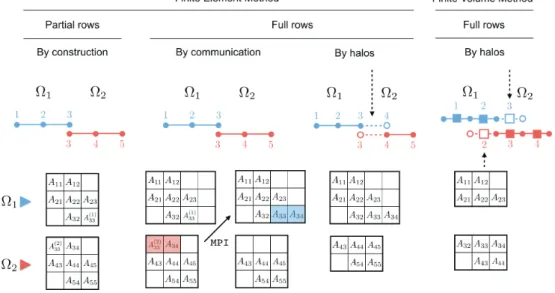
According to the partitioning described in the previous section, there exist three main ways of assembling the local matricesAð Þi of each subdomainΩi, as illustrated inFigure 5. The choice

for one or another depends on the discretization method used, on the parallel data structures required by the algebraic solvers (Section 5.2), but also sometimes on mysterious personal or historical choices. Let us consider the example ofFigure 5.

Partial row matrix.Local matrices can be made of partial rows (square matrices) or full rows (rectangular matrices). The first option is natural in the finite element context, where partitioning consists in dividing the mesh into disjoint element sets for each MPI process, and where only interface nodes are duplicated. In this case, the matrix rows of the interface nodes of neighboring subdomains are only partial, as its coefficients come from element integrations, as illustrated in

Figure 5(1) by matricesAð Þ₃₃1 andAð Þ₃₃2. In next section, we show how one can take advantage of this format to perform the main operation of iterative solvers, namely the sparse matrix vector product (SpMV).

Full row matrix.The full row matrix consists in assigning rows exclusively to one MPI process. In order to obtain the complete coefficients of the rows of interface nodes, two options are

Figure 5.Finite element and cell-centered finite volume matrix assembly techniques. From left to right: (1) FE: Partial rows, (2) FE: Full rows using communications, (3) FE: Full rows using halo elements, and (4) FV: Full rows using halo cells.

available in the FE context, as illustrated by the middle examples ofFigure 5: (1) by communi-cating the missing contributions of the coefficients between neighboring subdomains through MPI messages and (2) by introducing halo elements. The first option involves additional communications, while the second option duplicates the element integration on halo elements. In the first case, referring to the example ofFigure 5(2), the full row of node 3 is obtained by communicating coefficientsAð Þ₃₃2 from subdomainΩ2toΩ1. If the full row is obtained through

the introduction of halo elements, a halo element is necessary to fully assemble the row of node 3 in subdomain 1 and the row of node 4 in subdomain 2, as illustrated inFigure 5(3). The relative performance of partial and full row matrices depends on the size of the halos, involving more memory and extra computation, compared to the cost of additional MPI communications. Note that open-source algebraic solvers (e.g., MAPHYS [22], PETSC [23]) admit the first, second or both options and perform the communications internally if required. In cell-centered FV methods, the unknowns are located in the cells. Therefore, halo cells are also necessary to fully assemble the matrix coefficients, as illustrated byFigure 5(4). This is the option selected in practice in FV codes, although a communication could be used to obtain the full row format without introducing halos on both sides (only one side would be enough). In fact, let us imagine that subdomain 1 does not hold the halo cell 3. To obtain the full row for cell 2, a communication could be used to pass coefficientA23from subdomain 2 to subdomain 1.

Partial vs. full row matrix:

Load balance.As far as load balance is concerned, the partial row method is the one which a priori enables one to control the load balance of the assembly, as elements are not duplicated. On the other hand, in the full row method, the number of halo elements depends greatly upon the partition. In addition, the work on these elements is duplicated and thus limits the scal-ability of the assembly: for a given mesh, the relative number of halo elements with respect to interior elements increases with the number of subdomains.

Hybrid meshes.In the FE context, should the work load per element be perfectly predicted, the load balance would only depend on the partitioner efficiency (see Section 3). However, to obtain such a prediction of the work load, one should know the exact relative cost of assem-bling each and every type of element of the hybrid mesh (hexahedra, pyramids, prisms, and tetrahedra). This is a priori impossible, as this cost not only depends on the number of operations, but also on the memory access patterns, which are unpredictable.

High-order methods.When considering high-order approximations, the situations of the FE and FV methods differ. In the first case, the additional degrees of freedom (DOF) appearing in the matrix are confined to the elements. Thus, only the number of interface nodes increases with respect to the same number of elements with a first-order approximation. In the case of the FV method, high-order methods are generally obtained by introducing successive layer of halos, thus reducing the scalability of the method.

Sparse matrix vector product.As mentioned earlier, the main operation of Krylov-based iterative solvers is the SpMV. We see in next section that the partial row and full row matrices lead to different communication orders and patterns.

4.2. Shared memory parallelization using OpenMP

The following is explained in the FE context but can be translated straightforwardly to the FV context. Finite element assembly consists in computing element matrices and right-hand sides (Aeandbe) for each elemente, and assembling them into the local matrices and RHS of each MPI processi, namelyAð Þi andbð Þi. From the point of view of each MPI process, the assembly can thus be idealized as in Algorithm 1.

Algorithm 1Matrix Assembly in each MPI partitioni. 1:forelementsedo

2: Gather: copy global arrays to element arrays. 3: Computation: element matrix and RHSAe_,be_.

4: Scatter: assembleAe_,be_intoAð Þi_,bð Þi_.

5:end for

OpenMP pragmas can be used to parallelize Algorithm 1 quite straightforwardly, as we will see in a moment. So why this shared memory parallelism has been having little success in CFD codes?

Amdahl’s law states that the scalability of a parallel algorithm is limited by the sequential kernels of a code. When using MPI, most of the computational kernels are parallel by con-struction, as they consist of loops over local meshes entities such as elements, nodes, and faces, even though scalability is obviously limited by communications. One example of possible sequential kernel is the coarse grain solver described in Section 5.4. On the other hand, parallelization with OpenMP is incremental and explicit, making remaining sequential kernels a limiting factor for the scalability as stated by Amdahl’s law. This explains, in part, the reluctance of CFD code developers to rely on the loop parallelism offered by OpenMP. There exists another reason, which lies in the difficulty in maintaining large codes using this parallel programming, as any new loop introduced in a code should be parallelized to circumvent the so-true Amdahl’s law. As an example, Alya code [24] has more than 1000 element loops. However, the situation is changing, for two main reasons. First, nowadays, supercomputers offer a great variety of architectures, with many cores on nodes (e.g., Xeon Phi). Thus, shared memory parallelism is gaining more and more attention as OpenMP offers more flexibility to parallel programming. In fact, sequential kernels can be parallelized at the shared memory level using OpenMP: one example is once more the coarse solve of iterative solvers; another example is the possibility of using dynamic load balance on shared memory nodes, as explained in [25] and introduced in Section 4.3.

As mentioned earlier, the parallelization of the assembly has traditionally been based on loop parallelism using OpenMP. Two main characteristics of this loop have led to different algo-rithms in the literature. On the one hand, there exists arace condition. The race conditions comes from the fact that different OpenMP threads can access the same degree of freedom

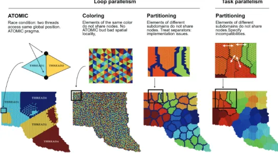
coefficient when performing the scatter of element matrix and RHS, in step 4 of Algorithm 1. On the other hand, spatial locality must be taken care of in order to obtain an efficient algorithm. The main techniques are illustrated inFigure 6and are now commented.

Loop parallelism using ATOMIC pragma. The first method to avoid the race condition consists in using the OpenMP ATOMIC pragmas to protect the shared variablesAð Þi andbð Þi

(Figure 6(1)). The cost of the ATOMIC comes from the fact that we do not know a priori when conflicts occur and thus this pragma must be used at each loop iteration. This lowers the IPC (defined in Section 1.2) that therefore limits the performance of the assembly.

Loop parallelism using element coloring.The second method consists in coloring [26] the elements of the mesh such that elements of the same color do not share nodes [27], or such that cells of the same color do not share faces in the FV context. The loop parallelism is thus applied for elements of the same color, as illustrated inFigure 6(2). The advantage of this technique is that one gets rid of the ATOMIC pragma and its inherent cost. The main drawback is that spatial locality is lessened by construction of the coloring. In [28], a comprehensive comparison of this technique and the previous one is presented.

Loop parallelism using element partitioning.In order to preserve spatial locality while dispos-ing of the ATOMIC pragma, another technique consists in partitiondispos-ing the local mesh of each MPI process into disjoint sets of elements (e.g., using METIS [18]) to control spatial locality inside each subdomain. Then, one definesseparatorsas the layers of elements which connect neighboring subdomains. By doing this, elements of different subdomains do not share nodes. Obviously, the

Figure 6.Shared memory parallelism techniques using OpenMP. (1) Loop parallelism using ATOMIC pragma. (2) Loop parallelism using element coloring. (3) Loop parallelism using element partitioning. (4) Task parallelism using partitioning and multidependences.

elements of the separators should be assembled separately [29, 30], which breaks the classical element loop syntax and requires additional programming (Figure 6(3)).

Task parallelism using multidependences.Task parallelism could be used instead of loop parallelism, but the three algorithmics presented previously would not change [30–32]. There are two new features implemented in OmpSs (a forerunner for OpenMP) that are not yet included in the standard that can help: multidependences and commutative. These would allow us to express incompatibilities between subdomains. The mesh of each MPI process is partitioned into disjoint sets of elements, and by prescribing the neighboring information in the OpenMP pragma, the runtime will take care of not executing neighboring subdomains at the same time [33]. This method presents good spatial locality and circumvents the use of ATOMIC pragma.

4.3. Load balance

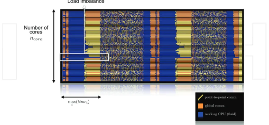
As explained in Section 1.2, efficiency measures the level of usage of the available computational resources. Let us take a look at a typical unbalanced situation illustrated in the trace shown in

Figure 7. Thex-axis is time, while they-axis is the MPI process number, and the dark grey color represents the element loop assembly (Algorithm 1). After the assembly, the next operation is a reduction operation involving MPI, the initial residual norm of the iterative solver (quite com-mon in practice). Therefore, this is a synchronization point where MPI processes are stuck until all have reached this point. We can observe in the figure that one of the cores is taking almost the double time to perform this operation, resulting in a load imbalance.

Load imbalance has many causes: mesh adaptation as described in Section 2.3, erroneous element weight prediction in the case of hybrid meshes (Section 3), hardware heterogeneity, software or hardware variabilities, and so on. The example presented in the figure is due to wrong element weights given to METIS partitioner for the partition of a hybrid mesh [28].

There are several works in the literature that deal with load imbalance at runtime. We can classify them into two main groups, the ones implemented by the application (may be using external tools) and the ones provided by runtime libraries and transparent to the application code.

In the first group, one approach would be to perform local element redistribution from neighbors to neighbors. Thus, only limited point-to-point communications are necessary, but this technique provides also a limited control on the global load balance. Another option consists in repartitioning the mesh, to achieve a better load distribution. In order for this to be efficient, a parallel partitioner (e.g., using the space filling curve-based partitioning presented in Section 3) is necessary in order to circumvent Amdahl’s law. In addition, this method is an expensive process so that imbalance should be high to be an interesting option.

In the second group, several parallel runtime libraries offer support to solve load imbalance at the MPI level, Charm++ [34], StarPU [35], or Adaptive MPI (AMPI). In general, these libraries will detect the load imbalance and migrate objects or specific data structures between pro-cesses. They usually require to use a concrete programming language, programming model, or data structures, thus requiring high levels of code rewriting in the application.

Finally, the approach that has been used by the authors is called DLB [25] and has been extensively studied in [28, 33, 36] in the CFD context. The mechanism enables to lend resources from MPI idle processes to working ones, as illustrated in Figure 8, by using a hybrid approach MPI + OpenMP and standard mechanisms of these programming models.

Figure 8. Principles of dynamic load balance with DLB [25], via resources sharing at the shared memory level. (Top) Without DLB and (bottom) with DLB.

In this illustrative example, two MPI processes launch two OpenMP threads on a shared memory node. Threads running on cores 3 and 4 are clearly responsible for the load imbalance. When using DLB, threads running in core 1 and core 2 lend their resources as soon as they enter the synchronization point, for example, an MPI reduction represented by the orange bar. Then, MPI process 2 can now use four threads to finish its element assembly.

Let us take a look at the performance of two assembly methods: MPI + OpenMP with loop

parallelism and MPI + OpenMP with task parallelism and dynamic load balance.Figure 9

shows the strong scaling and timings of these two methods. The example corresponds to the assembly of 140 million element meshes, with highly unbalanced partitions [33], as illustrated by the trace shown inFigure 7. As already noted in Section 1.2, although the strong scaling of the MPI + OpenMP with loop parallelism method is better than the other one, the timing is around three times higher. This is due to the combination of: substituting loop parallelism using coloring by task parallelism, thus giving a higher IPC; using the dynamic load balance library DLB to improve the load balance at the shared memory level.

4.4. More HPC optimizations

Let us close this section with some basic HPC optimizations to take advantage of some hardware characteristics presented in Section 1.1.1.

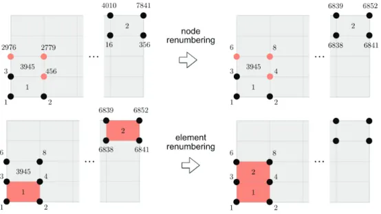
Spatial and temporal localityThe main memory access bottleneck of the assembly depicted in Algorithm 1 is the gather and scatter operations.Figure 10illustrates the concept. On the top figure, we illustrate the action of node renumbering [37, 38] to achieve a better data locality: nodes are“grouped”according their global numbering [37, 38]. For example, when assem-bling element 3945, the gather is more efficient after renumbering (top right part of the figure) as nodal array positions are closer in memory. Data locality is thus enhanced. However, the assembly loop accesses elements successively. Therefore, when going from element 1 to 2, there is no data locality, as element 1 accesses positions 1,2,3,4 and element 2 positions 6838,

Figure 9.Strong speedup and timings of two hybrid methods: MPI + OpenMP with loop parallelism and MPI + OpenMP with task parallelism and DLB, on 1024 to 16,384 cores.

6841, 6852, 6839. Therefore, renumbering the elements according to the node numbering enables one to achieve temporal locality, as shown in the bottom right part of the figure. Data already present in cache can be reused (data of nodes 3 and 4).

Vectorization.According to the available hardware, vectorization may be activated as a data-level parallelism. However, the vectorization will be efficient if the compiler is able to vectorize the appropriate loops. In order to help the compiler, one can do some“not-so-dirty”tricks at the assembly level. Let us consider a typical element matrix assembly. Let us denote

nnodeandngausas the number of nodes and Gauss integration points of this element;

Ae, Jac, and N are the element matrix, the weighted Jacobian, and the shape function, respectively. In Fortran, the computation of an element mass matrix reads:

do ig = 1,ngaus do jn = 1,nnode

do in = 1,nnode

Ae(in,jn) = Ae(in,jn) + Jac(ig) * N(in,ig) * N(jn,ig) end do

end do end do

This loop, part of step 3 of Algorithm 1, will be carried out on each element of the mesh. Now, let us define Ne, a parameter defined in compilation time. In order to help vectorization, last loop can be substituted by the following.

Figure 10.Optimization of memory access by renumbering nodes and elements. (1) Top: satial locality. (2) Bottom: temporal locality.

do ig = 1,ngaus do jn = 1,nnode

do in = 1,nnode

Ae(1:Ne,in,jn) = Ae(1:Ne,in,jn) + Jac(1:Ne,ig) * N(1:Ne,in,ig) * N(1: Ne,jn,ig)

end do end do end do

thus assembling Ne elements at the same time. To have an idea of how powerful this technique can be, in [39], a speedup of 7 has been obtained in an incompressible Navier–Stokes assembly with Ne = 32. Finally, note that this formalism can be relatively easily applied to port the assembly to GPU architectures [39].

5. Algebraic system solution

5.1. Introduction

This section is devoted to the parallel solution of the algebraic system

Ax¼b, (1)

coming from the Navier–Stokes equation assembly described in last section. The matrix and the right-hand side are distributed over the MPI processes, the matrix having a partial row or full row format.

As explained in last section, the assembly process is embarrassingly parallel, as it does not require any communication (except the case illustrated inFigure 5(b)). The algebraic solvers are mainly responsible for the limitation of the strong and weak scalabilities of a code (see Section 1.2). Thus, adapting the solver to a particular algebraic system is fundamental. This is a particularly difficult task for large distributed systems, where scalability and load balance enter into play, in addition to the usual convergence and timing criteria.

In this section, we do not derive any algebraic solver, for which we refer to Saad’s book [40] or [41] for parallelization aspects, but rather discuss their behaviors in a massively parallel context. The section does not intend to be exhaustive, but rather to expose the experience of the authors on the topic.

The main techniques to solve Eq. (1) are categorized as explicit, semi-implicit and implicit. The explicit method can be viewed as the simplest iterative solver to solve Eq. (1), namely a preconditioned Richardson iteration:

xkþ1_¼xk_þδtM1_bAxk_,

¼xk_þδtM1_rk_, (2)

whereM is the mass matrix,δtthe time step, andkthe iteration/time counter. In practice, matrixAis not needed and only the residualrk_{is assembled. High-order schemes have been}

presented in the literature such as Runge–Kutta methods, but from the parallelization point of view, all the methods require a single point-to-point communication in order to assemble the residualrk_{or alternatively the solutionx}kþ1_{if halos are used.}

Semi-implicit methods are mainly represented by fractional step techniques [42, 43]. They generally involve an explicit update of the velocity, such as Eq. (2) and an algebraic system with an SPD matrix for the pressure. Other semi-implicit methods exist, based on the splitting of the unknowns at the algebraic level. This splitting can be achieved for example by extracting the pressure Schur complement of the incompressible Navier–Stokes Eqs. [44]. The Schur complement is generally solved with iterative solvers, which solution involves the consecutive solutions of algebraic systems involving unsymmetric and symmetric matrices (SPD for the pressure). These kinds of methods have the advantage to extract better conditioned and smaller algebraic systems than the original coupled one, at the cost of introducing an addi-tional iteration loop to converge to the monolithic (original) solution.

Finally, implicit methods deal with the coupled system (1). In general, much more complex solvers and preconditioners are required to solve this system than in the case of semi-implicit methods. So, in any case, we always end up with algebraic systems like Eq. (1).

We start with the parallelization of the operation that occupies the central place in iterative solvers, namely the sparse matrix vector product (SpMV).

5.2. Parallelization of the SpMV

Let us consider the simplest iterative solver, the so-called simple or Richardson iteration, which consists in solving the following equation fork¼0,1,2…until convergence:

xkþ1_¼xk_þbAxk_{: (3)}

The parallelization of this solver amounts to that of the SpMV (sayy¼Ax) and depends on whether one considers the partial row or full row format, as illustrated inFigure 11.

SpMV for partial row matrix with MPI.When using the partial row format, the local result of the SpMV (in each MPI process) is only partial as the matrices are also partial on the interface, as explained in Section 4. By applying the distributive property of the multiplication, the results of neighboring subdomains add up to the correct solution on the interface:

y₃¼A32x2þA33x3þA34x4, ¼ A32x2þAð Þ331x3 þ Að Þ₃₃2x3þA34x4 , ¼yð Þ31 þy 2 ð Þ 3 :

In practice, the exchanges ofyð Þ₃1 andy₃ð Þ2 betweenΩ1andΩ2are carried out through the MPI

function MPI_Sendrecv. In the case, a node belongs to several subdomains, and all the neighbors’ contributions should be exchanged. Note that with this partial row format, due to the duplicity of the interface nodes, the MPI messages are symmetric in neighborhood (a subdomain is a neighbor of its neighbors) and size of interfaces (interface ofiwithjinvolves the same degrees

of freedom as that ofjwithi). Finally, let us note that the same technique is applied to compute the right-hand sides, as b3¼bð Þ31 þb

2 ð Þ

3 . After this matrix and RHS exchange, the solution of

Eq. (3) is therefore the same as in sequential.

SpMV for full row matrix with MPI.For this format, where all local rows are fully assembled and matrices are rectangular, the exchange is carried out before the local products on the multiplicands x3 and x4, as shown in Figure 11. The exchanges are carried out using

MPI_Sendrecv, which in the general case and contrary to the partial row format are no longer symmetric in size. Nothing needs to be done with the RHS as it has been fully assembled through the presence of halos.

Asynchronous SpMV with MPI.The previous two algorithms are said to be synchronous, as the MPI communication comes before or after the complete local SpMV for the partial or full row formats, respectively. The use of nonblocking MPI communications enables one to obtain asynchronous versions of the SpMV [41]. In the case of the partial row format, the procedure would consist of the following steps: (1) perform the SpMV for the interface nodes; (2) use nonblocking MPI communications (MPI_Isend and MPI_Irecv functions) to exchange the results of the SpMV on interface nodes; (3) perform the SpMV for the internal nodes; (4) synchronize the communications (MPI_Waitall); and (5) assemble the interface node contribu-tions. This strategy permits to overlap communication (results of the SpMV for interface nodes) and work (SpMV for internal nodes).

SpMV with OpenMP.The loop parallelization with OpenMP is quite simple to implement in this case. However, care must be taken with the size of the chunks, as the overhead for creating the threads may be penalizing if the chunks are too small. Another consideration is the matrix format selected such as CSR, COO, ELL. For example, COO format requires the use of an ATOMIC pragma to protecty.

Load balance.In terms of load balance, FE and cell-centered FV methods behave differently in the SpMV. In the FV method, the degrees of freedom are located at the center of the elements. The partitioning into disjoint sets of elements can thus be used for both assembly and solver. In the case of the finite element, the number of degrees of freedom involved in the SpMV corresponds to the nodes and could differ quite from the number of elements involved in the assembly. So the question of partitioning a finite-element mesh into disjoint sets of nodes may be posed, depending on which operation dominates the computation. As an example, if one balances a hexahedra subdomain with a tetrahedra subdomain in terms of elements, the latter one will hold six times more elements than the last one.

5.3. Krylov subspace methods

The Richardson iteration given by Eq. (7) is only based on the SpMV operation. SpMV does not involve any global communication mechanism among the degrees of freedom (DOF), from one iteration to the next one. In fact, the result for one DOF after one single SpMV is only influenced by its first neighbors, as illustrated byFigure 12(1). To propagate a change from one side of the domain to the other, we thus need as many iterations as number of nodes between both sides, that is1=h, wherehis the mesh size.

Krylov subspace methods, represented by the GMRES, BiCGSTAB, and CG methods among others, construct specific Krylov subspaces where they minimize the residualr¼bAxof the equation. Such methods seek someoptimality, thus providing a certain global communication mechanism. These parameters are functions of scalar products that can be computed locally on each MPI process and then assembled through reduction operations using the MPI_Allreduce function in the case of MPI, and the REDUCTION pragma using OpenMP. Nevertheless, this global communication mechanism is very limited and the convergence of such solvers degrades with the mesh size. Just like the Richardson method, Krylov methods damp high-frequency errors through the SpMV, but do not have inherent low-high-frequency error damping.

Figure 12.Accelerating iterative solvers. From top to bottom: (1) SpMV has a node-to-node influence; (2) domain decomposition (DD) solvers have a subdomain-to-subdomain influence; and (3) coarse solvers couple the subdomains.

The low-frequency damping can be achieved by introducing a DD preconditioner and/or a coarse solver, as is introduced in next subsection.

5.4. Preconditioning

The selection of the preconditioning of Eq. (1) is the key for solving the system efficiently [45, 46]. Preconditioning should provide robustness at the least price, for a given problem, and in general, robustness is expensive. Domain decomposition preconditioners provide this robust-ness, but can result too expensive compared to smarter methods, as we now briefly analyze.

Domain Decomposition.Erhel and Giraud summarized the attractiveness of domain decom-position (DD) methods as follows:

One route to the solution of large sparse linear systems in parallel scientific computing is the use of numerical methods that combine direct and iterative methods. These techniques inherit the advantages of each approach, namely the limited amount of memory and easy parallelization for the iterative component and the numerical robustness of the direct part.

DD preconditioners are based on the exact (or almost exact) solution of the local problem to each subdomain. In brief, the local solutions provide a coupling mechanism between the subdomains of the partition, as illustrated inFigure 12(2) (note that the subdomain matrices

Aiare not exactly the local matrices in this case). The different methods mainly differentiate in the way the different subdomains are coupled (interface conditions) and in terms of overlap between them, the Schwarz method being the most famous representative. On the one hand, SpMV is in charge of damping high frequencies. On the other hand, DD methods provide a communication mechanism at the level of the subdomains. The convergence of Krylov solvers using such preconditioners now depends on the number of subdomains.

Coarse solvers try to resolve this dependence, providing a global communication mechanism among the subdomains, generally one degree of freedom per subdomain. The coarse solver is a

“sequential”bottleneck as it is generally solved using a direct solver on a restricted number of MPI processes. Let us mention the deflated conjugate gradient (DCG) method [47] which provides a coarse grain coupling, but which can be independent of the partition.

As we have explained, solvers involving DD preconditioners together with a coarse solver aim at making the solver convergence independent of the mesh size and the number of subdomains. In terms of CPU time, this is translated into the concept of weak scalability (Section 1.2). This can be achieved in some cases, but hard to obtain in the general case.

Multigrid solvers or preconditioners provide a similar multilevel mechanism, but using a different mathematical framework [48]. They only involve a direct solver at the coarsest level, and intermediate levels are still carried out in an iterative way, thus exhibiting good strong (based on SpMV) and weak scalabilities (multilevel). Convergence is nevertheless problem dependent [49, 50].

Physics and numerics based solvers.DD preconditioners are brute force preconditioners in the sense that they attack local problems with a direct solver, regardless of the matrix

properties. Smarter approaches may provide more efficient solutions, at the expense of not being weak scalable. But do we really need weak scalability to solve a given problem on a given number of available CPUs? Well, this depends. Let us cite two physical/numerical-based preconditioners. The linelet preconditioner is presented in [51]. In a boundary layer mesh, a typical situation in CFD, the discretization of the Laplacian operator tends to a tridiagonal matrix when anisotropy tends to infinity (depending also on the discretization technique), and the dominant coefficients are along the direction normal to the wall. The anisotropy linelets consist of a list of nodes, renumbered in the direction normal to the wall. By assembling tridiagonal matrices along each linelet, the preconditioner thus consists of a series of tridiagonal matrices, very easy to invert.

Let us also mention finally the streamwise linelet [52]. In the discretization of a hyperbolic problem, the dependence between degrees of freedom follows the streamlines. By renumbering the nodes along these streamlines, one can thus use a bidiagonal or Gauss–Seidel solver as a preconditioner. In an ideal situation where nodes align with the streamlines, the bidiagonal preconditioner makes the problem converge in one complete sweep.

These two examples show that listening to the physics and numerics of a problem, one can devise simple and cheap preconditioners, performing local operations.

Figure 13illustrates the comments we have previously made concerning the preconditioners. In this example, we solve the Navier–Stokes equations together with ak-eturbulence model to simulate a wind farm. The mesh comprises 4 M nodes, with a moderate boundary layer mesh near the ground. The figure presents the convergence history in terms of number of iterations and time for solving the pressure equation (SPD) [53], with four different solvers and preconditioners: CG for Schur complement preconditioned by an additive Schwarz method; the DCG with diagonal preconditioner; the DCG with linelet preconditioner [51]; and the DCG with a block LU (block Jacobi) preconditioner. We observe that in terms of robustness (Figure 13

(1)) the additive Schwarz is the most performant solver, as it converges in six times less iterations than the DCG with diagonal preconditioner. However, taking a look at the CPU time, the performance is completely inverted and the best one is the DCG with linelet preconditioner. We

10-3 10-2 10-1 100 101 0 100 200 300 400 500 600 Residual Number of iterations Add. Schwarz DCG DCG linelet DCG block LU 10-3 10-2 10-1 100 101 0 2 4 6 8 10 12 Residual Time Add. Schwarz DCG DCG linelet DCG block LU

Figure 13. Convergence of pressure equation with 512 CPUs using different solvers (4 M node mesh). (1) Residual norm vs. number of iterations. (2) Residual norm vs. time.