“© 2014 IEEE. Personal use of this material is permitted. Permission from IEEE must be obtained for all other uses, in any current or future media, including
reprinting/republishing this material for advertising or promotional purposes, creating new collective works, for resale or redistribution to servers or lists, or reuse of any copyrighted component of this work in other works.”
An Infinite Adaptive Online Learning Model for
Segmentation and Classification of Streaming Data
Ava Bargi, Richard Yi Da Xu, Massimo Piccardi
Faculty of Engineering and IT, University of Technology, Sydney
PO Box 123 Broadway NSW 2007 Australia
Ava.Bargi,YiDa.Xu,[email protected]
Abstract—In recent years, the desire and need to understand streaming data has been increasing. Along with the constant flow of data, it is critical to classify and segment the observations on-the-fly without being limited to a rigid number of classes. In other words, the system needs to be adaptive to the streaming data and capable of updating its parameters to comply with natural changes. This interesting problem, however, is poorly addressed in the literature; as many of the common studies focus on offline classification over a pre-defined class set. In this paper, we propose a novel adaptive online system based on Markov switching models with hierarchical Dirichlet process priors. This infinite adaptive online approach is capable of segmenting and classifying the streaming data over infinite classes, while meeting the memory and delay constraints of streaming contexts. The model is further enhanced by a ‘predictive batching’ mechanism, that is able to divide the flowing data into batches of variable size, imitating the ground-truth segments. Experiments on two video datasets show significant performance of the proposed approach in frame-level accuracy, segmentation recall and precision, while determining the accurate number of classes in acceptable computational time.
I. INTRODUCTION AND RELATED WORK
The joint problem of time segmentation and recognition of streaming data into meaningful sub-sequences has attracted significant research in a variety of domains. The ability to automatically classify data segments and identify their tem-poral boundaries is a core technology for applications in speaker diarization, finance, activity understanding, multime-dia annotation and human-computer interaction. To date, the main solutions proposed have included the hidden Markov model [1], conditional random fields [2] [3], and structural SVM [4], covering the spectrum of generative, discriminative and maximum-margin dynamic classifiers. Also unstructured approaches such as bag-of-features have reported remarkable results [5]. Along with advancements in learning and inference, research has witnessed increasingly realistic datasets which are bridging the gap between lab and real applications [6] [7]. Nevertheless, important challenges intrinsic to real applications remain unresolved. We address three of these limitations, jointly in an online adaptive model that can accommodate an unlimited (i.e., theoretically infinite) number of classes.
The main limitation addressed in this paper is the lack of a learning approach for segmentation and recognition of streaming data that keeps on learning throughout the entire life of its application (online learning). Most of the related studies follow an offline approach that learns from a finite sequence of data [6] [7]. This obviously does not suit the needs of streaming data, which are ubiquitous in real-time applications.
Processing of streaming data has to be provided in anonlineor recursivemanner, with a limited memory buffer and tolerable delay between data acquisition and processing. In addition, the majority of the approaches have considered closed, pre-defined sets of classes. Such an assumption fails in scenarios such as long-term learning or monitoring, where the possible number of classes is not precisely predictable. Ultimately, as more data streams in, the known classes may evolve due to observing more comprehensive data or a natural evolution over time. In either case, models are expected to update parameters of the known classes through what we note as an ‘adaptive online learning’scheme. We have further enhanced the model by introducing an efficient predictive segmentation plug-in, noted as Conditional Factor Regression (CFR). CFR is inspired by [8] and [9], yet simplified for computational efficiency. As the data flow in, CFR splits the sequence into batches of variable size, aiming for each batch to contain a whole meaningful segment (e.g. activity) from start to end. The time efficiency and performance of this simple and innovative plug-in is analysed later plug-in the paper.
Amongst the many paradigms available for class mod-elling, hierarchical Bayesian modelling and, in particular, the hierarchical Dirichlet process (HDP) [10] offers a principled way to infer an arbitrary number of classes from a set of samples via a hierarchy of prior distributions. The hierarchical Dirichlet process (HDP) is a Bayesian nonparametric technique estimating the joint posterior distribution of a set of latent classes and a set of parameters, typically by Gibbs samplers [11] or variational inference [12]. It has been used for a variety of applications, including the modelling of sequential data by Markov switching models such as HDP-HMM [13]. In this case, the classes correspond to the discrete states of a Markov chain and the data are explained by a state-conditional observation model. Given a set of samples, classification is performed by decoding the states of the Markov chain. The Dirichlet process, its hierarchical successor and mixture models are increasingly applied to various domains, such as bio-informatics and vision (see [14], [15] for some recent references).
In this paper, we propose a novel adaptive online version of HDP-HMM suited for on-the-fly time segmentation and recog-nition of streaming data. The main contributions of this model are i) dividing the streaming data into batches of variable size, aiming to contain a full segment in each batch by utilising an efficient predictive batching method; ii) continuous posterior adaptation of parameters in each batch justified by the observed data, merely using a limited memory buffer. Unlike the similar
infinite online studies such as [16], the proposed model is fully automated and does not rely on human intervention. It is also considered as a one-pass process of streaming data, i.e. no revision is needed. These constraints obviously make adaptation much more challenging, but suited to more real-life problems. The closest reference to our approach is [17] which presented online inference for latent Dirichlet allocation, the closed-set counterpart of the Dirichlet process, over an unbounded buffer. Our work extends that model to infinite class sets while meeting the finite memory requirements of streaming data processing. The experimental results over two datasets (a stitched version of the Weizmann human action recognition dataset [18], and the assistive kitchen dataset from Technische Universit¨at M¨unchen [7]) give evidence of significant classification and segmentation performance.
The rest of this paper is organised as follows: in Section II we describe the hierarchical Dirichlet process and its temporal extension HDP-HMM. Section III presents the proposed online approach including the predictive batching plug-in. Through the experiments and discussions in Section IV, we evaluate and compare the proposed variants, followed by the Conclusion (section V).
II. THE HIERARCHICALDIRICHLET PROCESS
A Dirichlet process, DP(γ, H(λ)), is a generative model that can be thought of as a distribution over discrete distribu-tions with countably infinite categories. It is controlled by a scalar parameter,γ, known as the concentration parameter, and a base measure,H(λ). A sampleG0 from a Dirichlet process
is a distribution overθ, the space of the base measure, differing from zero at only a countably infinite number of locations, or atoms, θk, k= 1. . . K: G0∼DP(γ, H(λ)) : G0(θ) = K X k=1 βkδ(θ−θk), K→ ∞ θk∼H(λ), β∼GEM(γ) (1)
The discrete set of locations is obtained by repeatedly sampling the base measure, H(λ), while the weight for each location,
βk, k = 1. . . K, is established by a stick-breaking process, noted as GEM(γ) [19]. Ahierarchical Dirichlet process(HDP) consists of (at least) two layers of Dirichlet processes, with similar construction and weights noted asπj:
G0∼DP(γ, H(λ)) Gj= K X k=1 πjkδ(θ−θk) K→ ∞ θk∼H(θ), πj ∼DP(α, β), β∼GEM(γ) (2)
whereγandαare the concentration parameters of the respec-tive Dirichlet processes. The continuous space of distribution
H is taken to be the parameter space for a data likelihood, as in y ∼f(y|θ) : θ ∼H(λ). The likelihood f(y|θ) could be, for instance, a Gaussian distribution of mean parametersθ, sampled from a Normal-Inverse-Wishart distribution,H.G0is
discrete and composed of distinct atoms with probability one, and the variousGj,j= 1. . . J, are also discrete and sampled from the elements of G0. In other words, HDP requires the
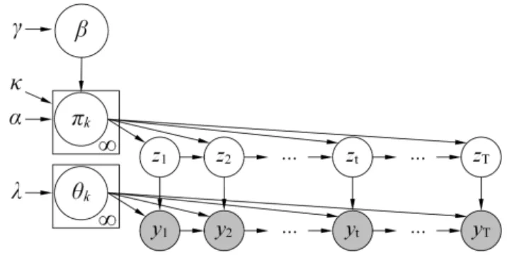
Fig. 1. HDP-HMM graphical model. The box notation is used to show replication.
data to belong to groups. Yet, rather than building an inde-pendent Gj model for each group, the hierarchical structure of the HDP allows the Gj to usefully share distributional properties. Examples can be as diverse as words in a book and genetic markers in a population. After the construction of the HDP, the generative model for the data is obtained from the Gj by sampling their weights via an indicator variable,
zj:zj∼πj, yj ∼f(y|θzj).
A. The HDP-HMM
The HDP has also been used by Teh et al. [10] and Fox et al. [13] as prior distribution for the parameters of switching models such as the hidden Markov model. When applied to a Markov chain, z1:T, p(z1:T) = p(z1)Q
T
t=2p(zt|zt−1), the
HDP changes its interpretation significantly (Figure 1). In this case, eachπj ={πjk},k= 1. . . K, is used as one row of the Markov chain’s transition matrix, representing the probability of transitioning from statej in the previous time-step to any other states in the current time-step, p(zt|zt−1 =j). Thanks
to the properties of HDP, new states will be created when the data are not properly explained by the current set of states. In contrast to the conventional HDP, the index of the group, j, of each observation is not known explicitly anymore, but it is instead inferred in sequential order from the chain. Therefore, in the case of the HDP-HMM zt ∼ p(zt|zt−1 = j) =
πj, yt ∼ f(yt|θzt). As a consequence, in the HDP-HMM
the number of groups (J) and the number of indices in each
πj (K) coincide. Adding the HDP as prior caters for arbitrary number of states, or activity classes [13].
It is worth adding that a reported limitation of HDP-HMM is the tendency to over-segment due to its unbounded number of classes [20]. Foxet al. have proposed adding a “sticky” prior to the transition matrix to emulate an inertia towards changing states, illustrated in Figure 1 [21]. We utilize the stickyprior in this study, yet denoting it as HDP-HMM for brevity. B. Inference and Learning
Inference and learning are typically performed simultane-ously in the HDP and its extensions by estimating the joint posterior distribution of the indicator variables, parameters, hidden variables and hyper-priors conditioned on the observa-tions. Deriving such an extensive joint posterior is analytically intractable, hence mainly inferred using Gibbs sampling or variational inference. Gibbs sampling is a simple yet effective
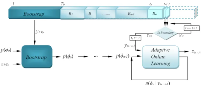
Fig. 2. Adaptive online learning flowchart, including the predictive batching plug-in (named as ‘Is Boundary’).
method capable of estimating complex posteriors with signifi-cant accuracy, yet it can converge slowly or have poor mixing. Variational inference is usually faster, however it can suffer from low accuracy due to approximation. Unlike the negative presumption about Gibbs efficiency, we will show how a brief initial supervised learning can result in substantially rapid convergence to highly accurate distributions.
Having inferred the class indicators,z1:T, we proceed with translating the indices into meaningful classes. In unsupervised learning, the correspondence between the ground-truth classes of the data and the labels assigned by the classification algorithm may not be obvious. In the case of the HDP, this problem is exacerbated by the fact that the number of classes is undetermined. Therefore, to re-establish the best possible one-to-one correspondence, the Hamming distance between ground-truth and assigned labels is minimised by a greedy algorithm, matching labels in decreasing frequency order.
III. THE ADAPTIVE ONLINEHDP-HMM
The proposed infinite adaptive online model enjoys a supervised initialisation prelude (bootstrap) of Tb frames, followed by the main unsupervised adaptive online phase that is potentially never-ending (Figure 2). In applications like activity recognition where annotation is easy, the bootstrap can be longer to provide a more comprehensive training; while in domains with costly annotation the initial training can be brief. In either case, during supervised learning, indicator variables
z1:Tb are fixed to their ground-truth values, and the model’s
parameters are sampled for a given number of iterations to reach convergence. After conclusion of the bootstrap phase, the data are processed in multiple batches, and the posterior probabilities of both indicator variables and parameters are estimated iteratively on each batch.
Considering a generic stream of data, y1:t, the posterior probability of the parameters can be written as p(φ|y1:t) ∝
f(y1:t|φ)p(φ), where φ indicates the vector of the generic parameters in Figure 1. The online version leverages on posterior adaptation, using the posterior computed up to time
t, as the prior for the next batch of data, yt+1:t+∆t
p(φn|y1:t+∆t)∝f(yt+1:t+∆t|φn−1, y1:t)p(φn−1|y1:t) ≈f(yt+1:t+∆t|φn−1)p(φn−1)
(3) wherenis the batch number. Given that the updated posterior embeds the distributional properties of the observations up to the current time, observations y1:t in Equation (3) can
(a) Batches of constant size
(b) Batches of segment size
Fig. 3. Two batching alternatives on a single instance of streaming data. Each color represents a ground-truth segment: (a) Fixed size batching, versus (b) predictive batching.
be discarded after adaptation. The non-parametric nature of the model is therefore confined to the current data batch, limiting memory requirements. While this may come at a price of reduced accuracy, to our knowledge it is the only viable approach for unbound streaming data. Such posterior adaptation is inevitable for learning infinite actions and refining the parameters, as aimed at the proposed system. However, the common unresolved challenge with adaptive learning systems is parameter drift over time. To mitigate this, we use a learning rate to balance the weight of the prior and that of the likelihood for the current data batch (see [22]).
A. Predictive batching
The posterior adaptation in Equation 3 is reliant on both the prior and likelihood. The former carries what the model has learnt from the initial training and the adaptive learning so far (y1:t), whereas the latter is governed by the observations in the current batch (yt+1:t+∆t). In a temporal model like HMM, a data sequence is best estimated when observed as a whole, from the first frame to the last. This will best comply with the transition probabilities of the frames within a class, compared to an observation batch that is a “mixed bag”, possibly including parts of multiple segments (see Figure 3(b) vs (a)). To leverage on this batching effect, we attempt to divide the streaming sequenceon-the-fly, into batches that contain full segments. Obviously, precise boundary prediction is a separate problem and what we propose hereafter is a method offering a fast and reasonably accurate decision on the next boundary, through predicting the next observation given the current and thresholding the prediction error.
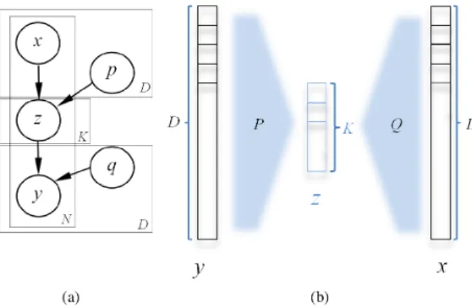
Since features are usually high-dimensional (especially in computer vision), predicting the next observation features given the current can be computationally costly and prone to over-fitting. We propose a simple and efficient regression model, that includes a low-dimensional intermediary latent factor, z, between the D-dimensional input x and response
y. Adding z contributes in two different ways: (a) bridging the input and response by decoupling their noise models, also (b) jointly reducing their ranks to K D to predict faster and avoid over-fitting (Figure 4).
p(y|z) =N(y|Qz, I),
p(z|x) =N(z|P x, I) (4)
wherexandyare high-dimensional input and response feature vectors, Q and P are factor loading matrices and identity
Fig. 4. Predictive batching by conditional factor regression (CFR): (a) The graphical model (b) The schematic diagram.
covariance matrices are utilised to model noise. Q and P
are learnt once during the bootstrap phase using Expectation-Maximisation (algorithm 1), and utilised later for every frame in the unsupervised phase. Marginalising z from Equation 4 results in a predictive scheme for y that only depends on the learnt Qand P: y˜=QP x. In our auto-regressive predictive batching scenario, input and response are two consecutive frame features, allowing us to predict the next feature using the current:y˜t+1=QP yt. After observingyt+1 we calculate
the error |y˜t+1 −yt+1| and threshold it with an empirical
measure. If the error is greater than the threshold for any given frame, there is a high chance that it belongs to a new segment. Therefore, the current batch is terminated atyt−1 and inferred
separately. Experimental results in Section IV is evidence of the usefulness and efficiency of this batching algorithm.
Algorithm 1:Predictive batching algorithm
Input: X1:Tb, Y1:Tb, K Output:Q, P
Initialise:QandP are P CA-initialised by the topK
columns of eig(cov(Y))andeig(cov(X)), respectively.
foriteration = 1 to ConvergenceMax do // E step: fori=1 toTbdo E[zi|Y, X] = (I+QTQ)−1(QTY +P X) E[zizTi|Y, X] = (I+QTQ)−1+E[zi|Y, X]E[zi|Y, X]T end // M step: P = PTb i=1E[zi|Y, X].x T i .(XXT)−1 Q= PTb i=1yi(E[zi|Y, X])T . PTb i=1E[zizTi|Y, X] −1 end
return QandP for predictingy given x.
IV. EXPERIMENTS
The simulation of the proposed model is inspired by the HDP-HMM Toolbox from Fox [23]1. As validation, we
1The code for our adaptive online HDP-HMM will soon be available online.
have used leave-one-out cross validation, using the training sequences as the bootstrap phase. To evaluate the results more comprehensively, metrics for both classification and time segmentation accuracies are reported. The classification accuracy is reported using frame level accuracy (Hamming distance), while time segmentation is gauged by the standard metrics of precision and recall for the detection of boundaries between two successive actions. A true boundary is regarded as correctly detected if a change of state is decoded within an interval of ±10 frames from the ground-truth location, due to annotation subjectivity. Any additional boundaries are instead counted as false positives. We also report the difference between the overall number of actions detected in the test sequence and the number of actions in the ground truth (denoted ascardinalityhereafter).
The following sections compare experiment results on a few variants of the proposed model. To our knowledge, there is no joint segmentation and recognition model conducting infinite adaptive onlinelearning to be fairly used as a bench-mark. Nevertheless, we use an offline run of our model (with a single batch containing the whole data) for comparison purposes. Although adaptive online processing, and the infinite number of classes introduce further complexities compared to the state-of-the-art studies, the proposed model performs remarkably well. To gauge the performance of the ‘predictive batching’ method, we compare the online model with a fixed-size batching variant (abbreviated as F ixBtch), an ’Oracle’ that divides the sequence based on ground-truth segments as the upper-bound batching accuracy (noted asOrclBtch) and ultimately the proposed predictive batching model using CFR (P redBtch).
A. Experiments on the stitched Weizmann dataset
The Weizmann dataset contains 93 single-action videos from a set of 10 action classes performed by 9 different actors. For action recognition alone, the Weizmann dataset is saturated [24] [25]. However, some major studies have collated its individual actions into a single (unsegmented) sequence to experiment with time segmentation [4], as a flexible way of creating multiple sequences. In our collation, we have created 4 action sequences with total length of 30 individual actions, randomly selected from the span of 10 action classes. As feature set, we have used the position of the actor’s centroid in the image plane and the distances between the centroid and the actors’ contour along five given directions.
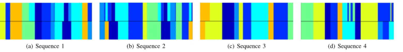
The estimated states of the adaptive online HDP-HMM variants over 4 sequences of the stitched Weizmann dataset are visualised in Figure 5, showing remarkable qualitative accuracy in segmentation and classification. The quantitative results are reported in Table I. The italic results noted as
Of f line variant represent the offline run of our model for the sake of comparison with a similar max-margin study [4], shown on the first row. Although the performances are on the same level, results are not directly comparable. Because datasets are similar in conception, yet different in sequence collation. In addition, the classifier in [4] worked over a closed set of classes, as opposed to our infinite scheme that allows unlimited number of classes. Table I is evidence of the proposed model’s excellent performance in inferring the right number of states.
The other variants represent the performance on fixed batches, as well as the predictive batching scheme. Please note that the batch size in F ixBtch is the average action length of the training data to provide a fair comparison with the predictive batching (P redBtch) variant. The OrclBtch
variant is a desirable oracle benchmark on the performance of our model with variable batch sizes, using the ground truth segments. As can be seen, the results of the predictive batching variant are very similar to the oracle, giving evidence of the reliability of the predictive batching method. In general, the predictive batching method improves the segmentation precision up to 15 percent, maintaining a similar frame-level accuracy compared to the fix batches (Table I).
B. Experiments on the TUM kitchen dataset
The TUM kitchen dataset is a useful human assistive dataset, consisting of natural unsegmented sequences of every-day activities performed in a typical kitchen environment [7]. The dataset contains multi-modal data, annotated separately for the actors’ left and right hands (9 classes) and trunk (2 classes). The main actions include ‘Reaching’, ‘Releasing Grasp Of Something’, ‘Taking An Object’, ‘Reaching Up-ward’, ‘Lowering An Object’, opening and closing doors and drawers and ‘Carrying While Locomoting’, the distinction of which are quite subtle at times even for human annotators. The main advantage of this dataset over the stitched Weizmann is that the transitions between actions occur naturally and time segmentation is more challenging.
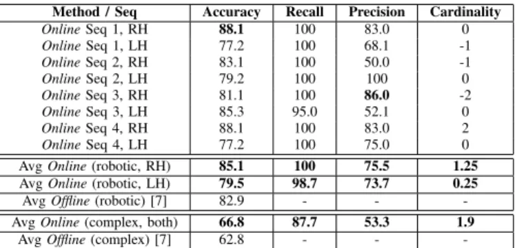
In our experiments, we have performed segmentation and classification on the actions of the left and right hands, separately. All the sequences provided with 3D motion capture features are used in the leave-one-out cross validation tests, also separately considered for the typical sequences (numbers 1-4, denoted as ‘robotic’), and the more challenging ones (‘complex’ sequences 5-21). Figure 6 plots the decoded states for the right and left hands on sequences 1 and 3 using the ‘predictive batching’ variant (P redBtch), showing significant qualitative match in frame-level accuracy, boundary detection and segmentation precision. The cardinality of inferred states are mostly correct. The quantitative results in Table II support this claim, outperforming a CRF benchmark study on the same dataset[7], both on robotic and complex sequences. We have reported the average figures for the complex sequences, due to lack of space. To calculate the average state cardinality error, we have utilised the absolute values for more clarity.
Similarly to the stitched Weizmann, the predictive batching scheme (P redBtch) improves the segmentation precision, while maintaining the same accuracy level as the oracle and fixed-size batching. It is important to mention that the predic-tive variant also improves the efficiency, decoding a sequence of around 1800 frames in an average of 50 seconds (36 frame per second), which is highly desirable and slightly more than real-time (the usual 30 frame per second rate in videos)2. This could be due to i) the efficient way of dividing the whole sequence into appropriate number of batches (predictive batching) and ii) as a result of the initial bootstrap, the Gibbs 2The experiments are run on a basic machine with an Intel i5 (3.10 GHz) processor and 4GB memory
Method / Seq Accuracy Recall Precision Cardinality OnlineSeq 1, RH 88.1 100 83.0 0 OnlineSeq 1, LH 77.2 100 68.1 -1 OnlineSeq 2, RH 83.1 100 50.0 -1 OnlineSeq 2, LH 79.2 100 100 0 OnlineSeq 3, RH 81.1 100 86.0 -2 OnlineSeq 3, LH 85.3 95.0 52.1 0 OnlineSeq 4, RH 88.1 100 83.0 2 OnlineSeq 4, LH 77.2 100 75.0 0 AvgOnline(robotic, RH) 85.1 100 75.5 1.25
AvgOnline(robotic, LH) 79.5 98.7 73.7 0.25
AvgOffline(robotic) [7] 82.9 - - -AvgOnline(complex, both) 66.8 87.7 53.3 1.9
AvgOffline(complex) [7] 62.8 - -
-TABLE II. FRAME-LEVEL ACCURACY,SEGMENTATION RECALL AND PRECISION,AND DIFFERENCE IN DECODED STATE CARDINALITY FOR
ONLINEHDP-HMM (P redBtch)ON ALLTUMKITCHEN DATASET.
method converges quite quickly (in less than 100 iterations), considerably decreasing the inference time for each batch3.
V. CONCLUSION
This paper has presented an adaptive online HDP-HMM for joint time segmentation and recognition of streaming data, over infinite sets of classes. Using posterior adaptation, the proposed online learning model is able to learn and adapt, using a constant memory buffer and minimal delay. Thanks to the properties of the hierarchical Dirichlet process, the number of states are flexibly inferred to adjust with the distribution of the streaming data. We have evaluated the proposed model over a few variants, particularly enhancing it with a predictive batching plug-in. This efficient boundary prediction mech-anism (denoted as conditional factor regression) is capable of estimating the segment boundaries, to thereby terminate a batch at the boundary points. Thanks to this property, segmentation precision is increased, maintaining the same accuracy with desirably shorter computational time. The ex-periment results on two datasets show remarkable frame-level accuracy, as well as segmentation recall (boundary detection) and precision (avoid over-segmentation). The inferred number of states match the ground-truth in most of the cases. The proposed model is not fairly comparable to existing studies on common datasets, due to having more degrees of freedom and observing the data in a streaming fashion, rather than all at once. However, the performance is remarkable, excelling the similar state-of-the-art studies.
REFERENCES
[1] J. Yamato, J. Ohya, and K. Ishii, “Recognizing human action in time-sequential images using hidden Markov model,” inProc. CVPR, 1992, pp. 379–385.
[2] C. Sminchisescu, A. Kanaujia, and D. Metaxas, “Conditional models for contextual human motion recognition,”Computer Vision and Image Understanding, vol. 104, no. 2-3, pp. 210–220, 2006.
[3] D. L. Vail, M. M. Veloso, and J. D. Lafferty, “Conditional Random Fields for Activity Recognition,” in Proc. Int. Conf. on Autonomous Agents and Multi-Agent Systems, 2007.
[4] M. Hoai, Z. Lan, and F. De la Torre, “Joint segmentation and classifi-cation of human actions in video,” inProc. CVPR, 2011.
[5] O. Duchenne, I. Laptev, J. Sivic, F. Bach, and J. Ponce, “Automatic an-notation of human actions in video,” inProceedings of the International Conference on Computer Vision (ICCV), 2009.
3A video demonstration of the adaptive online HDP-HMM can be found in http://www.youtube.com/watch?v=2PYYRrkUXIg
(a) Sequence 1 (b) Sequence 2 (c) Sequence 3 (d) Sequence 4
Fig. 5. Estimated states with the adaptive online HDP-HMM (FixBtch) for Weizmann dataset. Action labels are represented by colors. In each of the four illustrations, the horizontal axis is the time and the estimated labels are plotted on top of the true labels, providing a qualitative measure for the segmentation and classification performance. The respective quantitative figures are shown in Table I. This figure is better viewed in colour.
Accuracy Recall Precision Cardinality Method S1 S2 S3 S4 S1 S2 S3 S4 S1 S2 S3 S4 S1 S2 S3 S4 OfflineMax-margin [4] 87.7 (avg) - - -
-Adaptive OnlineHDP-HMM (Offline) 82.0 77.1 94.1 82.0 100 100 100 100 73.2 55.1 82.3 40.1 0 0 0 0 Adaptive OnlineHDP-HMM (FixBtch) 83.0 76.2 95.0 81.2 100 100 100 100 79.3 55.2 75.1 38.5 0 0 2 0
Adaptive OnlineHDP-HMM (PredBtch) 83.5 75.4 95.2 81.4 100 100 100 100 79.4 55.3 90.2 42.5 0 0 0 0
Adaptive OnlineHDP-HMM (OrclBtch) 83.0 75.1 95.4 81.3 100 100 100 100 79.5 55.4 90.2 50.2 0 0 0 0
TABLE I. FRAME-LEVEL ACCURACY,SEGMENTATION RECALL AND PRECISION,AND DIFFERENCE IN DECODED STATE CARDINALITY FOR THE ADAPTIVE ONLINEHDP-HMMVARIANTS AND STATE-OF-THE-ART STUDIES ON THE STITCHEDWEIZMANN DATASET.
(a) Sequence 1, LH (b) Sequence 1, RH (c) Sequence 3, LH (d) Sequence 3, RH
Fig. 6. Estimated states for the TUM kitchen dataset using the adaptive online HDP-HMM, with predictive batching (P redBtch). LH and RH stand for left and right hand.
[6] P. Over, G. Awad, M. Michel, J. Fiscus, W. Kraaij, and A. F. Smeaton, “Trecvid 2011 – an overview of the goals, tasks, data, evaluation mechanisms and metrics,” inProceedings of TRECVID 2011. NIST, USA, 2011.
[7] M. Tenorth, J. Bandouch, and M. Beetz, “The TUM Kitchen Data Set of Everyday Manipulation Activities for Motion Tracking and Action Recognition,” in IEEE International Workshop on Tracking Humans for the Evaluation of their Motion in Image Sequences (THEMIS), in conjunction with ICCV2009, 2009.
[8] L. Bo and C. Sminchisescu, “Supervised spectral latent variable mod-els,” inInternational Conference on Artificial Intelligence and Statistics, vol. 246, 2009, p. 248.
[9] A. Bargi, R. Y. D. Xu, and M. Piccardi, “A non-parametric conditional factor regression model for high-dimensional input and response,” CoRR, vol. abs/1307.0578, 2013.
[10] Y. W. Teh, M. I. Jordan, M. J. Beal, and D. M. Blei, “Hierarchical Dirichlet processes,”Journal of the American Statistical Association, vol. 101, no. 476, pp. 1566–1581, 2006.
[11] S. Geman and D. Geman, “Stochastic relaxation, Gibbs distributions, and the bayesian restoration of images,”Pattern Analysis and Machine Intelligence, IEEE Transactions on, vol. PAMI-6, no. 6, pp. 721 –741, nov. 1984.
[12] Y. W. Teh, K. Kurihara, and M. Welling, “Collapsed variational infer-ence for HDP,” inAdvances in Neural Information Processing Systems (NIPS), vol. 20, 2008.
[13] E. Fox, E. Sudderth, M. Jordan, and A. Willsky, “Bayesian Nonparamet-ric Inference of Switching Dynamic Linear Models,”IEEE Transactions on Signal Processing, vol. 59, no. 4, pp. 1569–1585, 2011.
[14] M. Zanotto, D. Sona, V. Murino, F. Papaleo, and H. Kjellstrom, “Dirichlet process mixtures of multinomials for data mining in mice behaviour analysis,” inInternational Conference on Computer Vision Workshops (ICCVW), 2013 IEEE Computer Society Conference on, 2013, pp. 197–202.
[15] C. Zhang, E. Henrik, X. Gratal, F. Pokorny, and H. Kjellstrom, “Supervised hierarchical Dirichlet processes with variational inference,”
inInternational Conference on Computer Vision Workshops (ICCVW), 2013 IEEE Computer Society Conference on, 2013, pp. 254–261. [16] C. Loy, T. Hospedales, T. Xiang, and S. Gong, “Stream-based joint
exploration-exploitation active learning,” inComputer Vision and Pat-tern Recognition (CVPR), 2012 IEEE Conference on, 2012, pp. 1560– 1567.
[17] K. R. Canini, L. Shi, and T. L. Griffiths, “Online Inference of Topics with Latent Dirichlet Allocation,” inProc. AISTATS 2009, vol. 5, 2009, pp. 65–72.
[18] L. Gorelick, M. Blank, E. Shechtman, M. Irani, and R. Basri, “Actions as space-time shapes,”Transactions on Pattern Analysis and Machine Intelligence, vol. 29, no. 12, pp. 2247–2253, December 2007. [19] J. Sethuraman, “A constructive definition of Dirichlet priors,”Statistica
Sinica, vol. 4, pp. 639–650, 1994.
[20] E. Fox, E. Sudderth, M. Jordan, and A. Willsky, “Developing a tempered HDP-HMM for systems with state persistence,” MIT Laboratory for Information and Decision Systems, Tech. Rep., 2007.
[21] E. B. Fox, E. B. Sudderth, M. I. Jordan, and A. S. Willsky, “An HDP-HMM for systems with state persistence,” inProc. ICML, July 2008. [22] A. Bargi, R. Xu, and M. Piccardi, “An online hdp-hmm for joint
action segmentation and classification in motion capture data,” in Computer Vision and Pattern Recognition Workshops (CVPRW), 2012 IEEE Computer Society Conference on, 2012, pp. 1–7.
[23] E. B. Fox, “HDP-HMM toolbox, beta version,” 2009. [Online]. Available: http://stat.wharton.upenn.edu/ ebfox/software/
[24] L. Wang and D. Suter, “Recognizing human activities from silhouettes: Motion subspace and factorial discriminative graphical model,” inProc. CVPR. Los Alamitos, CA, USA: IEEE Computer Society, 2007. [25] L. Nanni, S. Brahnam, and A. Lumini, “Combining different local
binary pattern variants to boost performance,” Expert Systems with Applications, vol. 38, no. 5, pp. 6209 – 6216, 2011.