Testing the predictive ability of corridor implied volatility under GARCH models

(1)

Testing the predictive ability of corridor implied

volatility under GARCH models

Shan Lu

∗

November 2018

Abstract

This paper studies the predictive ability of corridor implied volatility (CIV) measure. It is motivated by the fact that CIV is measured with better precision and reliability than the model-free implied volatility due to the lack of liquid options in the tails of the risk-neutral distribution. By adding CIV measures to the modified GARCH specifications, the out-of-sample predictive ability of CIV is measured by the forecast accuracy of conditional volatility. It finds that the narrowest CIV measure, covering about 10% of the RND, dominate the one-day ahead conditional volatility forecasts regardless of the choice of GARCH models in high volatile period; as market moves to non volatile periods, the optimal width broadens. For multi-day ahead forecasts narrow and mid-range CIV measures are favoured in the full sample and high volatile period for all forecast horizons, depending on which loss functions are used; whereas in non turbulent markets, certain mid-range CIV measures are favoured, for rare instances, wide CIV measures dominate the performance. Regarding the comparisons between best performed CIV measures and two benchmark measures (market volatility index and at-the-money Black-Scholes implied volatility), it shows that under the EGARCH framework, none of the benchmark measures are found to outperform best performed CIV measures, whereas under the GARCH and NAGARCH models, best performed CIV measures are outperformed by benchmark measures for certain instances.

Keywords: Corridor implied volatility; GARCH models; Model-free implied volatility; Black-Scholes implied volatility.

I thank Xin Jin, and participants at the German Finance Association (DGF) Annual Meeting in October 2017 in Ulm, Germany, and the Forecasting Financial Markets Conference in May 2017 in Liverpool, UK, for comments on earlier versions of this paper.

This is a pre-print of an article published inAsia-Pacific Financial Markets. The final authenticated version and the supplementary material are available online athttps://doi.org/10.1007/s10690-018-9262-5.

(2)

1. Introduction

Forecasts of volatility are important for accessing and managing risks of portfolios of securities. Particularly, it has emerged that volatility measured by realized volatility indi-cators over future horizons is widely traded across various markets for a variety of financial assets. These volatility indicators are facilitated with the development of extracting market predictions of future volatility from option prices with the consensus that volatility implied by market prices of options is a well-informed prediction of underlying asset future volatility. Various methods for extracting volatility information from option prices have been pro-posed. The Black-Scholes implied volatility (BSIV) is obtained by inverting market prices of options via the Black-Scholes model. However, due to the multitude of BSIV, one is unable to get a single market prediction of future volatility given a panel of options. It was recognized that prices of some options may be more informative and less sensitive to market frictions, to this end, a natural choice is the at-the-money BSIV. Besides, it was also suggested that some weighting schemes of the BSIV may improve the forecast ability. Perhaps due to its ad hoc feature, BSIV enjoys little success in predicting volatility (see

Figlewski,1997). The model-free implied volatility (MFIV), introduced byCarr and Madan

(1998); Britten-Jones and Neuberger (2000), offers a way of obtaining what is meant by a single market prediction from a cross section of option prices. The MFIV, in principle, can be derived from a continuum of cross section of European call and put option prices by replicating the variance contract with the support of the entire risk-neutral distribution (RND). However, due to the data limitations, the computation of MFIV truncates the tails of the RND where no reliable option prices can be obtained. Given the inherent feature of the option data that the range of available option prices differs across trading days, the

de-gree of truncation varies stochastically over time (seeCBOE,2015). More recently, corridor

implied volatility (CIV), introduced by Carr and Madan (1998); Andersen and Bondarenko

(2007), fixes MFIV in this regard. Compared to MFIV, the computation of CIV extends

the tails of the RND in a reliable fashion so that the severity of the truncation is consis-tent over time. The computation of CIV only requires options with strike prices that lie inside pre-defined price barriers (termed as ”corridor”) without the need of the support of

the entire RND. Andersen, Bondarenko, and Gonzalez-Perez(2015) compares the behaviour

of high-frequency MFIV and CIV, and show that MFIV is severely biased due to artificial jumps caused by inconsistent truncations during turbulent periods.

CIV recognizes that different parts of the RND are estimated with different degrees of precision; it allows one to dissect the information of the entire RND into slices. By

(3)

the pattern of risk premiums for the upside and downside variance; Muzzioli (2013) show that downside implied volatility is a better forecast of downside variance than upside implied

volatility for the upside variance; Dotsis and Vlastakis (2016) show that only upside risk is

priced in cross-section stock returns and subsumes all the relevant information for volatility forecasting.

But selecting the most informative parts (corridor) of the RND to extract an efficient market forecast of underlying asset future volatility given a panel of option prices remains largely an empirical question. Besides, questions of how CIV measure is compared to BSIV and MFIV (represented by market volatility index) in terms of predictive ability are left open.

Several studies have analyzed the optimal corridor with which the constructed CIV

mea-sure is closest correlated to future realized volatility. Andersen and Bondarenko(2007) show,

for index options, that CIV is more correlated to future return volatility than MFIV, and

certain narrow CIV measure outperforms BSIV.Tsiaras (2010) compare CIV with different

corridors from a symmetric cut of the RND for individual stocks from DJIX 30 index and find that CIV measures with a wider corridor are better forecasts of future realized volatility

compared to both BSIV and MFIV. Muzzioli (2013) show, in line with the findings of

An-dersen and Bondarenko(2007), that for index options CIV measures with narrower corridors outperforms CIV measures with wider corridors.

In terms of methodology, while regression based methods for comparing the predictive content of implied volatility are popular among prior literature where implied volatility itself is interpreted as a forecast of future volatility, it is suggested that GARCH models provide a general framework for comparing the incremental information content of implied volatilities for both in-sample hypothesis testing and out-of-sample forecast accuracy test. The GARCH method adopts a more pragmatic view that implied volatility contains all relevant information necessary to form a market prediction of future volatility. By adding implied volatility into GARCH models as an exogenous variable, the predictive content of

implied volatility can be tested. Day and Lewis (1992) estimate the modified GARCH(1,1)

and EGARCH(1,1) specifications for the S&P 100 index without allowing the decay rates for conditional variance and implied volatility to differ, they find that both returns and implied volatility contains incremental information. The same GARCH specification is also used by Kroner, Kneafsey, and Claessens (1995) for the commodity markets where they reach a

similar conclusion. Xu and Taylor(1995);Guo(1996) also use a similar GARCH specification

for the currency options markets but with conditional generalized error distribution. More

recently, Blair, Poon, and Taylor (2001) use the modified TGARCH model to compare the

(4)

to specifications in prior studies, they allow the decay rates for conditional variance, implied volatility and intraday returns to differ, they find that VIX provides most accurate forecasts.

Similar approach is also used by Taylor, Yadav, and Zhang (2010) for the comparison of

predictive content of different (implied) volatility measures.

Since out-of-sample forecasting is more practical relevant than in-sample testing of hy-pothesis of the information content, the comparisons of forecasting performance in this paper is carried out in an out-of-sample context. Out-of-sample comparisons are included in most aforementioned studies under the GARCH framework. This is because the parameters of in-sample fitted GARCH models only characterize the within-sample properties of implied

volatility, in-sample predictive ability is not transferable to out-of-sample. Dimson and

Marsh (1990) show that the improvement of in-sample forecast ability due to data snooping

is not transferable to out-of-sample forecasting. Nelson (1992) show that ARCH models

provide good in-sample predictive performance even when the model is misspecified, but out-of-sample forecasting is poor.

By using the modified GARCH models incorporating CIV measures with different corri-dors, the paper, firstly, assesses the out-of-sample predictive ability of CIV measures through evaluating the forecast accuracy of out-of-sample conditional volatility. The out-of-sample

approach is similar to Blair et al. (2001) who apply the nested model constructed from the

modified TGARCH specification with implied volatility to out-of-sample forecasting, utiliz-ing information only from implied volatilities. This paper, instead of usutiliz-ing the nested model, employs the unrestricted model containing information from both index returns and implied volatilities. Besides, CIV measures are compared to two benchmark measures, BSIV and a market volatility index. Finally, a simple trading strategy is used to assess the economic significance of CIV measures.

Our empirical results show that the narrowest CIV measure, covering about 10% of the RND, dominate the one-day ahead conditional volatility forecasts regardless of the choice of GARCH models in high volatile period; as market moves to non volatile periods, the optimal width broadens. For multi-day ahead forecasts, narrow and mid-range CIV measures provide the most accurate conditional volatility forecasts in high volatility period and the full sample for all forecast horizons, whereas mid-range and certain broad CIV measures dominate non

turbulent regimes. Our results echoes those by Andersen and Bondarenko (2007); Muzzioli

(2013) for index options where they find CIV measures, covering about 50% of the RND,

are closest related future realized volatility for the forecast horizon of 21 days.

The paper is arranged as follows. Section 2 describes the data.Section 3 introduces the

volatility measures used in this paper. Methods for forecasting and evaluation are presented

(5)

the economic significance of competing implied volatility measures in a simulated options

market. Section 7concludes the paper.

2. Data

Data used in this paper are obtained from several sources. Daily end-of-day DJX options (underlying: Dow Jones Industrial Average) are obtained from the Chicago Board Options Exchange (CBOE). Daily DJIA index levels and dividend yields are downloaded from the

Thomson Reuters DataStream; The volatility index under the ticker symbol ”VXD”1 is

downloaded from the Federal Reserve Economic Data (FRED) of the Federal Reserve Bank of St. Louis. Option sample period is from October 1, 2004 to March 6, 2015. DJX options are European style, and have up to three near-term expiration months and up to three months on the March quarterly cycle (March, June, September and December), and may also have up to five years to maturity Leaps. Procedures of option data set construction are described in the Appendix.

Daily treasury yield curve (also called constant maturity treasury, CMT) rates are used as risk-free rates and are obtained from the Board of Governors of the Federal Reserve System. Various maturities, from one-month to thirty-year rates, are available. Interest rates with intermedia maturities are linearly interpolated, and interest rates with maturities that are beyond available ranges are estimated by a natural cubic spline extrapolation.

Mid bid-ask prices, instead of traded prices, are used as option prices to eliminate the bounce effect (Bakshi, Cao, and Chen,1997,2000), and the spread effect (Figlewski, 1997). Option’s time to maturity is calculated by the number of calendar days remaining to maturity

less one (Dumas, Fleming, and Whaley, 1998) for AM-expiration options.

3. Volatility Measures

3.1. Construction of CIV

Unlike MFIV which needs the support of the entire RND, CIV only captures a fraction

of the RND. For a pre-defined corridor/strike range (BL, BH), CIV is computed as

CIV(BH, BL) = 2erT T Z BH BL M0(K) K2 dK (1)

(6)

where M0(K) = min(C0(K), P0(K)) is the out-of-money European option price, C0(K) and

P0(K) denote the current prices of European call and put options with strike price K and

expiration dateT. BLandBH denote the lower and upper corridor bounds for the underlying

asset price.

Corridor implied volatility defined in Eq. (1) is numerically implemented by:

CIV(BL, BH) = erT T m X i=1 h g(Ki) +g(Ki−1) i ∆K (2) where g(Ki) = M0(Ki, T)/Ki2, ∆K = (BH − BL)/m, Ki = BL +i∆K, BL = R−1(pl),

BH =R−1(pu). R(·) is the empirical cumulative risk-neutral probability distribution (RND)

function. A large m (m = 6000) is chosen in order to eliminate the discretization error

(Jiang and Tian, 2005, 2007). Since the available strike price points are sparse, a natural

cubic spline interpolation and a linear extrapolation 2 of the implied volatility with respect

to options moneyness3 are used to obtain prices of options with unavailable strikes. Two

sets of options with maturities closest to 30 (calendar) days are used to construct the CIV measure: near-term options with maturities smaller than 30 days and next-term options with maturities larger than 30 days. CIV measures at the two maturities are linearly interpolated

to obtain a CIV measure over a 30-day horizon (CBOE, 2015).

Similar to Andersen and Bondarenko(2007), only a symmetric cut of the RND is

consid-ered to construct CIV measures, meaning that the lower and upper risk-neutral probabilities

satisfy pl +pu = 1. Eleven lower risk-neutral probabilities are chosen, pl = 0, 0.01, 0.05,

0.1, 0.15, 0.2, 0.25, 0.3, 0.35, 0.4, 0.45, and denote the respective eleven CIV measures as CIV0, CIV1, CIV5, CIV10, CIV15, CIV20, CIV25, CIV30, CIV35, CIV40, CIV45, with CIV0 the

broadest CIV measure, and CIV45 the narrowest CIV measure. For example, CIV20,

repre-sentingCIV(R−1₍₀_.₂₎_{, R}−1₍₀_._{8)), is a CIV measure computed with lower and upper corridor}

bounds corresponding to risk-neutral probabilities of 0.2 and 0.8, respectively. CIV0 can be

regarded as the corridor-fixed MFIV (Andersen et al., 2015).

The RND is extracted from a cross section of option prices and approximated by the ratio statistic, R(K) proposed by Andersen et al.(2015)

R(K) = P(K)

C(K) +P(K) (3)

whereC, P are call and put option prices, respectively. The method overcomes the drawbacks

of percentile-based methods, details are discussed in Andersen, Bondarenko, and

Gonzalez-2_See_{Jiang and Tian}₍₂₀₀₇_{) for explanations.}

(7)

Perez(2011). The statistic is a monotonically increasing function of the strike price. There-fore, for each chosen risk-neutral probability there must be a single corresponding strike price.

3.2. Other Volatility Measures

At-the-money Black-Scholes implied volatility (BSIV) is extracted from ATM option prices by inverting the Black-Scholes model. The 30-day at-the-money BSIV is obtained by linearly interpolating BSIVs obtained from prices of near-term and next-term options.

n-day realized volatility is calculated by the Parkinson’s estimator of Parkinson (1980):

n_σ2 RV,t = n X t=1 ln(High_t)−ln(Lowt) 4 ln(2) (4)

where Hight and Lowtare daily high and low DJIA index levels, respectively. The left

super-script n indicates the length of time horizon over which the realized volatility is calculated.

4. Forecasting Methodology

4.1. Model

The exponential GARCH (EGARCH) is employed since the EGARCH model has the advantage that it captures the stylized facts about return volatility such as the leverage effect and volatility clustering. Implied volatility measures are incorporated into the EGARCH, producing the following specification:

lnht= α0+α1zt−1+κ |zt−1| − q 2 π 1−βL + δlnσimp,t−2 1 1−βvL (5) zt= (rt−µ)/ p ht, zt∼i.i.d.(0,1)

where rt − µ is the excess index return with µ being the expected return, L is the lag

operator,α1 measures the sign effect and is typically negative, andκmeasures the size effect

and is typically positive,δ is the parameter that captures the in-sample information content

of the implied volatility measure. β and βv are volatility decay rates for the conditional

volatility and the option term, respectively; they are allowed to differ from each other sicne

the condition β = βv as assumed in the EGARCH specification in Day and Lewis (1992)

(8)

represented by implied volatility measures (CIV, VXD or BSIV).

By placing certain parameter restrictions on the model defined in Eq.(5), three different

models are obtained using different information sets:

1. a volatility model that uses daily index returns alone: δ = 0.

2. a volatility model that uses information contained in option prices without explicit use

of daily index returns: α1 =κ= 0.

3. the unrestricted model that uses information in both historical index returns and im-plied volatility.

We compared the in-sample volatility forecasting performance of aforementioned two

re-stricted models with the unrere-stricted model by a log-likelihood ratio test 4_{, and we found}

that the unrestricted model consistently outperform restricted models significantly at 1%

sig-nificance level; the parameterδ on the option term are significant at 5% significance level for

all CIV measures, indicating a significant information content of CIV measures in addition to the historical information in index returns. The unrestricted model is used in compar-ing the out-of-sample forecastcompar-ing performance. The model is estimated by maximizcompar-ing the

log-likelihood function with respect to the normal density 5 without parameter restrictions.

4.2. Forecasting Methods

Rolling-window forecast is employed to perform out-of-sample forecast of conditional variances of DJIA index returns. The model evaluation period is from January 3, 2006 to March 5, 2015 (2308 trading days), data from October 1, 2014 to December 30, 2015 (316 trading days) are used as pre-sample.

Over the evaluation period, at each forecast origin t, the n-day realized volatility nσ_RV,t2 is the variable to forecast by incorporating the implied volatility measure into the EGARCH

model. A total number of 2308 n-day ahead volatility forecasts nht are produced, where

n

ht is a forecast of nσRV,t2 based on the information ˆΨt−1,...,t−316 (6)

for trading days t =N + 1, ..., N +T, where N = 316 is the fixed length of the estimation

window, T = 2308 is the length of period for forecasting. ˆΨt−1,...,t−316 = ( ˆα0,αˆ1,β,ˆ βˆv,δˆ)0 is

4_{Results of in-sample volatility forecasting performance of restricted and unrestricted models are not}

reported.

5_{A student-t or a generalized error distribution might provide better performance than a normal}

dis-tribution does due to the observed leptokurtic distributed asset returns. However, since the information content of market volatility expectations are studied in the same model setting, the choice of the assumed density function is orthogonal to the ranking of the forecasting performance of different market volatility

(9)

the EGARCH model parameter estimates based on past 316 observations of index returns

and implied volatility. One-day ahead volatility forecast 1_h

t is given by 1 ht= exp ˆ α0+ ˆα1zt−1+ ˆκ |zt−1| − q 2 π 1−βLˆ + ˆ δlnσ_imp,t−2 ₁ 1−βˆvL ! (7)

Since only lag one implied volatility measure is available at each forecast origin, multi-day

ahead forecasts cannot be computed by dynamic forecast. Similar to Blair et al. (2001),

under the assumption that E(n_h

t|Ψt−1,...,t−316) =1 ht, to produce 5, 10 and 21 day volatility

forecasts, the one-day ahead volatility forecast is, respectively, multiplied by 5, 10 and 21,

n_h

t=1ht×n, n= 5,10,21 (8)

However, due to the stochastic feature of volatility, this multiplicative method for computing multi-day ahead conditional variance forecasts may handicap the forecasting performance of implied volatility measures, and may lead to a different ranking of forecasting performance compared to the ranking produced in the evaluation of one-day ahead forecast. The square-root-of-time rule for compounding short-term volatility for long-horizons are discussed and

empirically tested in Balaban and Lu(2016);Danielsson and Zigrand (2006);Diebold,

Hick-man, Inoue, and Schuermann (1998).

4.3. Forecast Evaluation

Let Mk denote the EGARCH model that incorporate implied volatility measure k, and

hk,t which is defined in Eq.(6) denote the volatility forecast obtained from modelMk. Model

Mk yields a sequence of forecasts, hk,1, ..., hk,T, that are compared to σ2RV,1, ..., σ2RV,T, using

a loss functionLk,t, for t=N+ 1, ..., N +T. Consequently, the matter for determining the

forecasting performance of implied volatility measures then relies on the evaluation criterion. Various forecasting criteria are considered in this paper for accessing the forecasting performance of an implied volatility measure. A number of loss functions are chosen and are

summarised in Table 1. These loss functions are considered by Patton (2010) and Hansen

and Lunde (2005). Particularly, the mean squared error (MSE) is robust in the presence of noise in the volatility proxy (Patton, 2010).

Besides, the serial correlation R2 _{obtained from the Mincer-Zarnowitz regression}

n

(10)

is also reported. It offers the proportion of variance explained by the best linear combination of α+β(n_h

t).

In addition, out-of-sample tests require a robust test statistic for determining the statis-tical significance of the forecasting performance. Once the test statistic is constructed, its statistical significance needs to be evaluated, probably by a bootstrap. There are a number of

candidate tests in the literature on out-of-sample forecasting. For instance, Hodrick (1992)

constructs a test statistic under a null hypothesis of no predictability; Goyal and Welch

(2008) uses the historical average return as a benchmark for evaluating forecast ability of

the index return; Diebold and Mariano (1995) and West (1996) focus on the framework of

testing for equal predictive ability (EPA), while White(2000) develops a framework (known

as the Reality Check) of testing for whether a particular forecast model or procedure is outperformed by alternative forecasts, representing a test of superior predictive ability. A

further development of this framework byHansen(2005) is known as the superior predictive

ability test (SPA). The SPA test has the advantage over the reality check of White (2000)

that SPA is less sensitive to the inclusion of poor and irrelevant alternative forecasts, and it

is more powerful than other alternative tests for accessing predictive ability (Hansen, 2005;

Hansen and Lunde, 2005). Therefore, this paper adopts the SPA test of Hansen (2005) to investigate the relative performance of various implied volatility measures under GARCH models.

The procedure of the SPA test of Hansen (2005) is briefly introduced below. Consider

K + 1 different implied volatility measures k for k = 0, ..., K, which then produces K + 1

EGARCH models Mk. Let M0 be the benchmark model that is compared to models k =

1, ..., K. Each model leads to a sequence of losses Li,k,tfor a particular choice of loss function

i, the relative performance variable can then be defined as

Xk,t ≡Li,0,t−Li,k,t, k = 1, ..., K, t=N + 1, ..., N +T. (10)

The null hypothesis is, in terms of the expected lossE(Xk,t), that the benchmark modelM0

does not underperform any alternative model Mk. Under the null hypothesis, the loss Li,0,t

obtained from benchmark modelM0 is no larger than the lossLi,k,tobtained from alternative

model Mk for all k = 1, ..., K, for a chosen loss functioni. Thus the null hypothesis can be

formulated as

(11)

where

λk ≡E(Xk,t). (12)

The test statistic for the SPA test ofHansen (2005) is given by

TSP A= max k=1,...,K √ TX¯k ˆ ωkk (13) where ¯Xk =T−1 PN+T

t=N+1Xk,t (the expected loss), ˆω2kk is the consistent estimator of ω

2

kk and

ω_kk2 = limT→∞var(

√

TX¯k). As suggested by Hansen (2005), the SPA test is implemented

based on the stationary bootstrap of Politis and Romano (1994). The bootstrap resamples

{X_b,∗₁, ..., X_b,K∗ }, b = 1, ..., B, are constructed by combining blocks of random lengths, and

block lengths are chosen to be geometrically distributed with mean q= 0.5. The number of

resamples B are chosen to be relatively large. The consistent estimator ˆωkk of ωkk can then

be computed using the bootstrap resamples:

ˆ ωkk = 1 B B X b=1 ( ¯X∗ b,k−X¯¯k∗)2 (14) where ¯X∗

b,k= _T1 PN_t₌+_NT₊₁Xb,k,t∗ (the sample mean of each bootstrap resample), ¯X¯k∗ = B1

PB

b=1X¯∗b,k. The empirical distribution of the test statistic for resamples

T_b∗ = max k=1,...,K √ TZ¯_b,k∗ ˆ ωkk , b= 1, ..., B (15)

converges to the distribution of the test statistic TSP A _{under the null hypothesis, with}

¯ Z_b,k∗ = ¯X∗ b,k−X¯¯k∗×1_X¯¯∗ k>−Ak, Ak = 1 4T −4_ω_ˆ

kk, 1{·} is the indicator function. The p-value can

then be computed p-value = 1 B B X b=1 1{T∗ b>TSP A}. (16)

The null hypothesis of the SPA test is rejected for small p-values. In the case whereTSP A_≤_0,

there is no evidence that the benchmark model underperforms all alternative models, by

convention p-value≡1. The SPA p-value is not a p-value in the conventional sense, the SPA

p-value can be interpreted as the intensity of the benchmark producing superior forecasts. A SPA p-value of 1 indicates the benchmark outperforms all alternatives.

(12)

4.4. Subsamples

The model evaluation period is divided into three ex-ante sub-periods: high volatility, medium volatility, and low volatility periods. These ex-ante sub-periods are chosen accord-ing to 21-(tradaccord-ing)day conditional volatility forecasts obtained from a GJR-GARCH(1,1) model estimated from historical DJIA index returns. The GJR-GARCH(1,1) model has the following specification:

ht=

α0+α12t−1 +θ2t−11{t−1 <0}

1−βL (17)

the one-step ahead 21-day volatility forecast is obtained by

σt,t+21 = s 252 21 h 21σ2₊1−φ 21 1−φ (ht+1−σ 2₎i ₍₁₈₎

where φ = α1 + 0.5θ+β (persistence parameter), σ2 = α0/(1−φ) (unconditional return

variance). Days with 21-day conditional volatility forecasts larger than 66.6 percentile of the volatility forecasts sample are included in high volatility period.

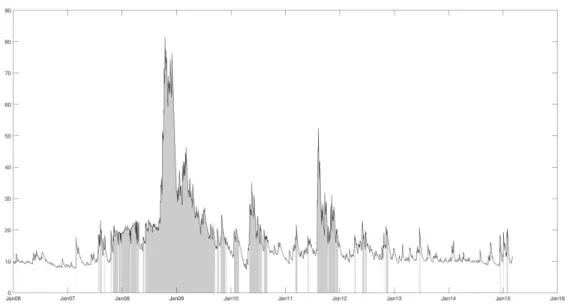
Figure 1 show the selected high volatility periods. It’s expected to be intermittent.

However, the high volatility period generally coincides with the public perception of periods of volatile markets such as the financial crisis from late 2007 to 2009, and the European Union’s sovereign credit issues in 2010.

5. Results

5.1. Descriptive Statistics

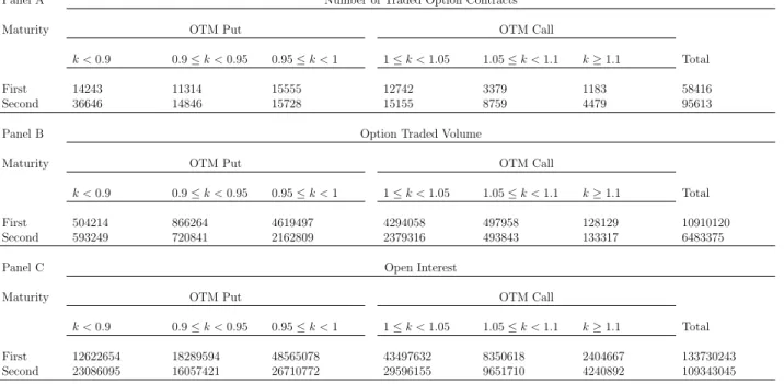
Table 2 reports the summary statistics for the option data sample. There are some patterns: (1) more put option contracts are traded than call option contracts, especially

for deep out-of-money (DOTM) contracts (k < 0.9 or K ≥ 1.1), implying that the market

provides insurance against extreme price movements over a broader price interval on the left side of the price distribution than on the right side. This is also reflected by the option

traded volume: the total traded volume for DOTM put options with moneyness k <0.9 is

almost four times as many as the traded volume of DOTM calls with moneynessk ≥1.1. (2)

Near-the-money (NTM) and at-the-money (ATM) (0.95≤ k < 1.05) options are the most

liquid options. For example, the total traded volume of NTM puts is almost nine times as many as the total traded volume of DOTM put options for the first maturity, and is more

(13)

than three times as many as the total traded volume of DOTM put options for the second maturity. The summary statistics for the open interest are in line with the findings above.

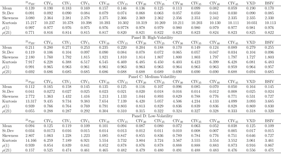
Table 3 reports various summary statistics for eleven CIV measures, VXD and BSIV over the full sample and three subsamples. Focusing on the full sample, VXD is compatible with

the level of the broadest CIV measure CIV0, they both exceed the level of realized volatility

by 36.7%. There is a monotonically decreasing pattern in the mean level of CIV measures as

corridor width narrows. The mean level of CIV15, covering only 70% of the RND, is 5% higher

than realized volatility. Narrower CIV measures are more stable than broader CIV measures in terms of higher serial auto-correlation, lower sample standard deviation, skewness and kurtosis. Realized volatility is more volatile than all implied volatility measures, it has the highest sample standard deviation, skewness and kurtosis statistics, and the lowest 21-day serial auto-correlation when measurement overlap has minimum effects. Concerning the at-the-money BSIV, the magnitude of BSIV is significantly lower than broad CIV measures and VXD. It is more persistent than broad CIV measures at both daily and monthly frequencies, and has lower skewness and kurtosis of all series. Note that for all measures the serial auto-correlation decay very slowly and can be well approximated by a hyperbolic shape, indicating there is a long memory component in the volatility process. The summary statistics for subsamples are consistent with the findings above.

5.2. One-Day Ahead Forecasting Performance

Table 4 reports the goodness-of-fit measure R2 and best performed CIV measure based

on the SPA test. The R2 _{is obtained from the Mincer-Zarnowitz regression as defined in}

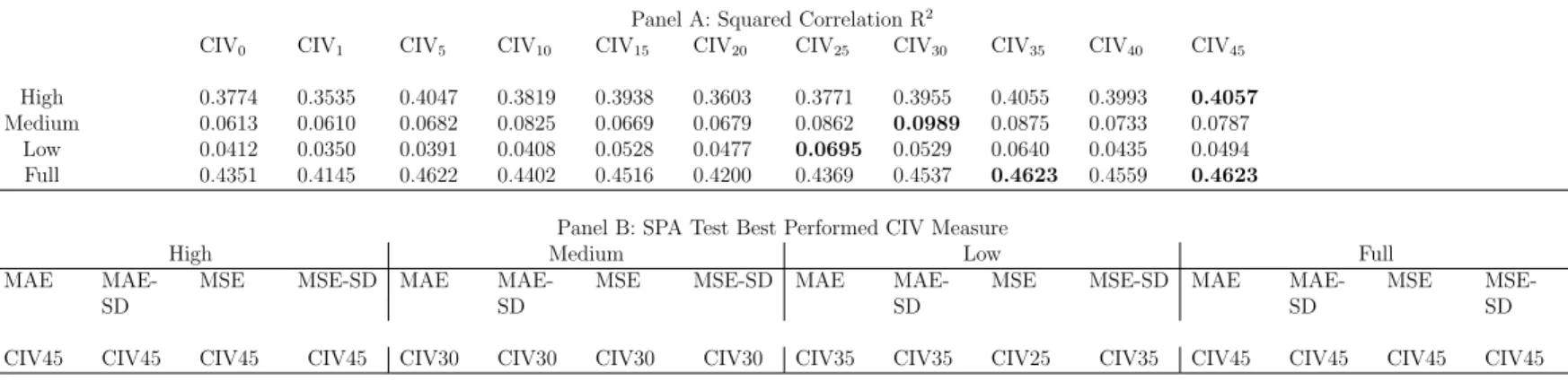
Eq.(9). R2 _{shows that in high-volatility period and the full sample, the pattern of one-day}

ahead forecasts obtained from EGARCH incorporating the narrowest measure (CIV45) is

closest to the pattern of one-day realized volatility itself compared to other CIV measures. The optimal corridor width broadens as the market moves from high volatility to medium and low volatility periods, covering 40% and 50% of the RND, respectively. On the other hand, best performed CIV measures are obtained via the SPA test under a null hypothesis that the benchmark CIV measure does not underperform any other CIV measures. The SPA test assesses wether same results can be obtained from similar samples. Therefore, it measures the statistical significance of results of our sample. All of the best performed CIV

measures have a SPA p-value of 1. The SPA results support the results from R2_{. Particularly,}

the results for MSE are consistently with R2_{, this is due to the fact that R}2 _{compares the}

sum of squared mean deviations of forecast errors. Different results are shown for the low

(14)

performance.

Broader CIV measures have larger total forecast errors than the narrowest CIV measure in high-volatility period, whereas they have smaller total errors in medium volatility and low

volatility periods (Table 11 in the supplemental material). For instance, compared to CIV45,

the disadvantages of CIV30 and CIV35 in high volatility periods offset their advantages in

medium and low volatility periods. The advantage of CIV45offsets its disadvantage in other

subsamples.

To compare the forecasting performance of CIV measures with other implied volatility measures, the forecasting procedure is repeated for the CBOE volatility index VXD (under-lying: DJIA index) and the ATM Black-Scholes implied volatility (BSIV).

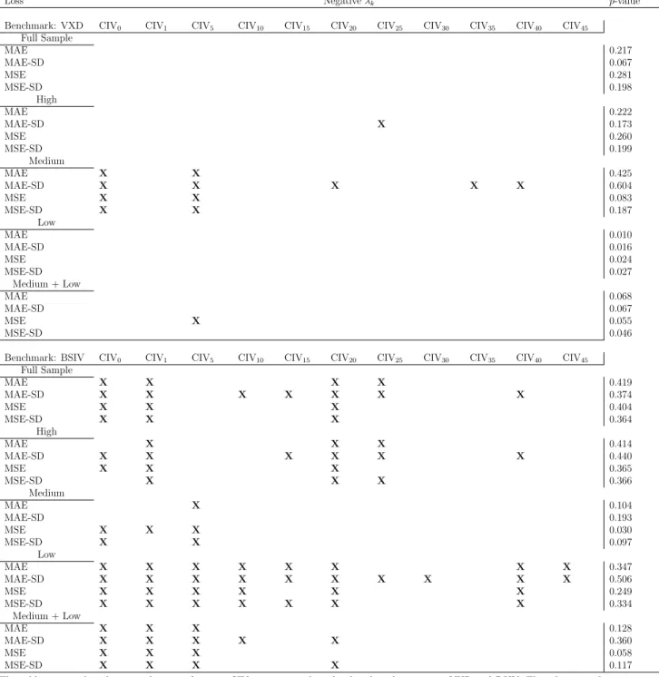
Table 5 reports the relative performance of the benchmark measure (VXD/BSIV) com-pared to CIV measures and SPA test p-values. The relative performance is measured by the

mean loss λk, only the sign of λk is reported. A negative λk indicates a superiority of the

benchmark measure over the alternative. P-values are obtained from the SPA test under a null hypothesis that the benchmark measure is not inferior to any CIV measures. Con-cerning VXD, results show that only in the medium volatility period, VXD outperforms two

broadest CIV measures (CIV0 and CIV5), and for rare instances, VXD outperforms narrow

CIV measures according to MAE-SD. For the full sample and all other subsamples, VXD is outperformed by CIV measures. Note that for periods excluding high volatility period, VXD

is outperformed by all CIV measures except CIV5 according to MSE. SPA p-values indicate

that VXD does not outperform all CIV measures.

Moving to the performance of BSIV, results show that BSIV outperforms two broadest CIV measures for almost all instances. Mid-range CIV measures are outperformed by BSIV in all subsamples and the full sample except the medium volatility period. Two narrowest CIV measures are outperformed in low volatility period, and in high volatility period and the full sample according to MAE-SD. For the periods excluding high volatility period, BSIV does not outperform narrow CIV measures. The p-values indicate that for all instances, BSIV does not outperform all CIV measures.

5.3. Multi-Day Ahead Forecasting Performance

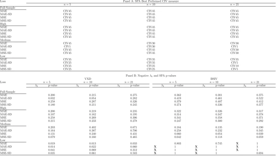
Moving to the performance of multi-day ahead forecasts, Table 6 reports forecasting performance for three forecasting horizons: 5, 10 and 21 days. Panel A shows the best performed CIV measures which obtained via the SPA test under a null hypothesis that the benchmark CIV measure does not underperform any other CIV measures. All of the best

(15)

other CIV measures in the full sample and high-volatility periods for all instances. This is similar to the pattern of one-day ahead forecasts. Yet, the narrowest CIV measure stays superior in terms of predictive ability in medium-volatility periods over 5- and 10-day forecast horizons according to MSE and MSE-SD, and over 5-day horizon according to MAE. For other instances in the medium-volatility periods and all instances in low-volatility periods, the SPA test favours broader CIV measures, covering 30 to 50% of the RND. However, there are some instances where broad CIV measures, covering about 80 to 98% of the RND, outperform others in medium- and low-volatility periods.

Panel B compares the performance of the benchmark measure (VXD/BSIV) with best

performed CIV measures. Relative performance measure λk and the SPA p-values are

re-ported. The SPA p-values are obtained from the SPA test under a null hypothesis that the

benchmark measure does not underperform any CIV measures. λkshows that VXD are

out-performed by CIV measures for all instances. All p-values are small, the null hypothesis of the SPA test for VXD is rejected. Concerning BSIV, for all instances in the full sample, high

and medium volatility periods, both λk and SPA test disfavours BSIV in terms of forecast

ability. In contrast, in low volatility periods, BSIV outperforms all CIV measures for three forecasting horizons, except for 21-day horizons according to MSE-SD, and 5- and 10-day horizons according to MAE.

5.4. Alternative Models

The forecasting procedure is repeated for two other frequently used GARCH family mod-els: namely GARCH and the nonlinear asymmetric GARCH (NAGARCH) with the following specifications respectively: GARCH: ht= α0+α12t−1 1−βL + δσ_imp,t−2 ₁ 1−βvL (19) NAGARCH: ht= α0+α1 t−1−θ p ht−1 2 1−βL + δσ2 imp,t−1 1−βvL (20)

5.4.1. One-Day Ahead Forecasts

Table 7 reports the one-day ahead forecasting performance of alternative models. Under

both GARCH and NAGARCH models, as suggested by R2_{, the narrowest CIV measure}

provides the most accurate out-of-sample one-day ahead forecasts for the full sample and high volatility period, and the optimal width broadens as market moves from high volatility period to medium and low volatility periods, covering 40 to 60% of the RND, except for

(16)

measure (CIV1). In addition, the results from R2 are consistent with the SPA test if MSE is used. The advantage of best performed CIV measure in high volatility period offsets its disadvantage in medium and low volatility periods, so that the best performed CIV measure for the full sample is the same as in high volatility period (Table 12 and 13 in the supplemental material). Those patterns support the results of EGARCH one-day ahead forecasts.

The results for comparisons with benchmark measures under alternative models are slightly different from results under EGARCH. Under GARCH, CIV measures are outper-formed by VXD only in medium volatility period if MAE and MAE-SD are used. For other periods, VXD is outperformed by best performed CIV measures. In contrast, under NA-GARCH, VXD does not outperform all CIV measures for all instances. Moving to BSIV, under GARCH, BSIV outperforms all CIV measures in medium volatility period, whereas it is outperformed by the best performed CIV measures for all other instances, except for the full sample and high volatility period if MSE is used. However, under NAGARCH, it is found that best performed CIV measures are outperformed by BSIV for the full sample and high volatility period, while CIV measures are able to deliver more accurate forecasts in medium and low volatility periods.

5.4.2. Multi-Day Ahead Forecasts

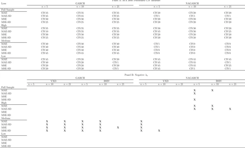
Table 8 reports the multi-day ahead forecasting performance for GARCH and NA-GARCH. Under GARCH, mid-range and narrow CIV measures are favoured for the full sample for all three horizons, covering 10 to 50% of the RND. Note that the best performed CIV measures for the full sample are almost the same as for high volatility period except for the loss function MAE-SD, this is similar to the pattern for results discussed in previous sec-tions. For the medium volatility period, all loss functions prefer two narrowest CIV measures for all three forecast horizons, whereas in low volatility period, mid-range and narrow CIV measures are preferred for horizons of 5 and 10 days, broader measures for 21-day forecast horizon. Under NAGARCH, no obvious patterns exist. However, for most instances in the full sample, high volatility and low volatility periods, SPA test favours mid-range and narrow CIV measures over broad measures with some exceptions. Two broadest CIV measures are preferred in medium volatility period.

Panel B shows the results for comparisons with the benchmark measure (VXD/BSIV). Under GARCH, best performed CIV measures are outperformed by VXD only in medium volatility period for horizons of 10 and 21 days, whereas they outperform VXD for all other instances. BSIV outperforms all CIV measures similarly in medium volatility period , but for 5 and 10-day horizons. BSIV are favoured for 21-day horizon if MSE is used in medium

(17)

best performed CIV measures. Under NAGARCH, similar patterns are presented for VXD, but only for 5-day horizon. However, different patterns are presented for BSIV under NA-GARCH. BSIV is found to be superior for the forecast horizon of 5 days in the full sample and high volatility period, and for 10-day horizon for high volatility period if MAE and MAE-SD are used. BSIV is also preferred for 10-day horizon if MAE is used in the full sample, and for 21-day horizon if MAE-SD is used in high volatility period. The mixed results of comparisons between best performed CIV measures and the benchmark measure

for multi-day ahead forecasts may be due to that the multiplicative method in Eq.(8) for

computing multi-day ahead forecasts under a constant volatility assumption contradicts with the fact that volatility is stochastic.

5.5. Corridor Bounds

Table 9 reports the percentage of days when corridor bounds are beyond the available strike range. The corridor bounds for the broadest CIV measure stay outside the available strike range for all the sample days. The percentage number decreases dramatically as corridor width narrows. It should be noted that the extrapolation used to compute broad CIV measures should not affect our results because: (1) a linear extrapolation ensures that the extrapolated prices are not under- (over) estimated for puts (calls); (2) corridor bounds for CIV measures covering 70% of the RND or less stay outside the available strike range on less than 1% of sample days, yet their out-of-sample performance differs, this is true especially for high volatility periods; (3) except for the narrowest CIV measure which provides consistent superior performance in high volatility periods, the optimal corridor width for medium and low volatility periods does change under different models: for instance, under

the NAGARCH, CIV1 outperforms narrower CIV measures in the medium volatility periods,

while on more than half of sample days the upper corridor bounds for the first maturity stay outside the available strike range.

6. Economic Significance

In this section, we examine the economic significance of various implied volatility mea-sures based on simulated options trading. Option strategies are constructed to only allow speculations on the volatility information. A simple delta-hedged put option strategy is used.

(18)

6.1. Simulated Trading

The trading is carried out ex ante (out-of-sample). On each trading day, market agents fit past 316 observations of CIV measures in a simple AR(1) model with the following specification:

lnCIVt =β0+β1lnCIVt−1+εt. (21)

The estimated parameters are used to forecast today’s CIV, and the CIV forecast is then used to obtain a price forecast for the ATM put options by using the Black-Scholes Model. Market agents enter their positions by buying (selling) one put contract if the option portfolio

is underpriced (overpriced), and simultaneously buying (selling) ∆p number of DJIA index

futures. The positions are closed by an offsetting order so that they can rebalance their portfolio the next day. Only options with maturities between 7 to 60 days are traded. Futures with a maturity closest to the put option are chosen. If a put option traded on the previous day cannot be found on the next day, the rate of return for that contract during this period is recorded as -1. The rate of return of the delta-hedged puts is calculated as, if an put contract is bought:

π = (Pclose−Popen) +|∆p|(Fclose−Fopen) Popen

(22)

and if an put option contract is sold:

π =−(Pclose−Popen) +|∆p|(Fclose−Fopen)

Popen

(23)

where P is the put option price, ∆p is the put option’s delta. Market agents are allowed

to borrow at the risk-free rate and to invest all profits from option trades into risk-free assets. Therefore, a risk-free rate are deducted (added) from (to) the rate of return of the

delta-hedged puts. p-values for the mean are based on Efron and Tibshirani (1993) and

Efron (1979), and p-values for the Sharpe ratio are based on Opdyke (2007). All p-values are calculated through a bootstrap t-test. The t-test is based on the empirical distribution of returns. The empirical distribution of returns is obtained from 10000 nonparametric bootstrap repetitions of the return sample. Each repetition is obtained by drawing daily rates of returns with replacement.

6.2. Before Transaction Costs

(19)

narrowest CIV has a significant mean return of 0.776% at 10% significance level. In the

medium volatility periods, measures from CIV20 to CIV45 have significant mean returns,

with a mean return of 1.1052% for CIV45, the highest among all significant mean returns.

In low volatility periods, no CIV measure is found to have significant mean returns. In the

full sample, CIV15, CIV30 and narrower CIV measures have significant means, with CIV45

possessing the highest significant mean return of 0.6305%. None of CIV measures have a significant Sharpe ratio.

The results of comparisons of mean returns and Sharpe ratios are reported in the supple-mental material (Table 14 and Table 15). They show that in the medium-volatility periods and the full sample, narrower CIV measures generate significant larger mean returns than broader CIV measures, VXD and BSIV at 10% significance level. No significant differences between mean returns are found in high volatility and low volatility periods. The profitability pattern of Sharpe ratios is similar to that of mean returns.

6.3. After Transaction Costs

Extensive literature has documented that transaction costs are quite substantial in the options market. Transaction costs mainly include two parts: the bid-ask spread and com-mission fees. The bid-ask spread reflects the supply and demand conditions in the options market, and is often seen to be quite small in a liquid market. We introduce a 25% effective

bid-ask spread6: the effective ask (bid) price is the midpoint price plus (minus) 12.5% of the

bid-ask spread. In addition, we also include a commission fee which is set to 0.5% of the value of the traded option portfolio; see (Hull, 2012, Table 9.1) for a typical commission fee scheme in the options market. Since we close out our positions in the options market by an offsetting order, commission fees are payable both upon entering and exiting the current position in the market. Results present similar patterns to before translaction costs, except that all CIV measures are found to generate significant losses under all market conditions. The results of trading after transaction costs are not reported in the paper.

7. Conclusion

This paper provides studies on the predictive ability of corridor implied volatility (CIV) measure. It is motivated by the fact that CIV is measured with better precision and reliability than the model-free implied volatility (MFIV) due to the lack of liquid options in the tails of

6_{In our unreported results, a larger or smaller effective bid-ask spread does not change the pattern of the}

(20)

the risk-neutral distribution (RND) (Andersen and Bondarenko,2007). By selecting different parts of the RND with pre-defined upper and lower price barriers (termed as ”corridor”), CIV measures with different corridors are constructed. The paper differs from prior research on CIV, in terms of methodology, that the predictive ability of CIV measures is evaluated through the out-of-sample forecast accuracy of conditional volatility, by adding CIV measures to the modified GARCH models.

Out-of-sample comparisons show, for the Dow Jones Industrial Average index, that the narrowest CIV measure, covering about 10% of the RND, provide the most accurate one-day ahead conditional volatility forecasts for the full sample and high-volatility period, regardless of the choice of GARCH models. It is also observed that the optimal corridor width broad-ens as market moves from high volatility regime to medium and low volatility regimes, with mid-range CIV measures dominate non volatile markets. Regarding the multi-day ahead forecasts, similar conclusions are reached: narrow and mid-range CIV measures, covering about 10 to 50% of the RND, are favoured in the full sample and high volatile period, de-pending on which loss functions are used; whereas certain wide and mid-range CIV measures are favoured in non turbulent markets. It is also find that since the advantage of the best performed CIV measure in high volatility period is large, it offsets its disadvantages in non turbulent times, the optimal CIV measures in the full sample is consistently in line with

in high volatility period. Our results echoes those by Andersen and Bondarenko (2007);

Muzzioli (2013) for index options where they find mid-range CIV measures, covering about 50% of the RND, are closest related future realized volatility for 21-day forecast horizon.

The comparisons between CIV measures and two market benchmark measures show that best performed CIV measures are occasionally outperfomed by the CBOE volatility index VXD only in medium volatility regimes. Whereas BSIV is found to outperform best performed CIV measures in high volatility period and the full sample under GARCH and NAGARCH framework, and is inferior to CIV measures under the EGARCH model.

The trading simulation shows that only the narrowest CIV measure is able to generate significant mean returns at 10% significance level before transaction costs. After transaction costs, none of the implied volatility measures are able to generate significant profits.

Appendix A.

Option Data Set Construction

This appendix provides a detailed description of the procedure of option data cleaning, since the raw option data are disorganized, and may contain stale price quotes and quotes that violate non-arbitrage conditions.

(21)

2. The underlying asset price is adjusted by deducting the cash dividends from the daily closing index levels. For DJIA index, daily actual dividends are not available, the dividend-adjusted prices are calculated by using daily dividend yield

S_i∗ =Sie−ζiτi

where S_i∗ is the dividend-adjusted index level, Si is the daily closing index level, ζi is the

daily dividend yield on day i, τi is options’ time to maturity (annualized).

3. Several option filters are applied to exclude stale option quotes. These quotes are generated by options that are illiquid and likely mispriced. The filters are:

(1) Options with zero-bid quotes are excluded from the sample.

(2) Options with less than 7 days time to maturity are excluded. These options are illiquid and are affected by microstructure factors.

(3) In-the-money options are excluded. In-the-money options are generally overpriced and are less liquid than ATM and OTM options. Both OTM put and call options are used in order to ensure the range of the available strikes is sufficiently wide, and this will minimize the approximation errors due to extrapolation in BSIV at strikes beyond the available strikes.

(4) Options that violate basic non-arbitrage conditions are excluded. Non-arbitrage con-ditions for European options include boundary concon-ditions, monotonic concon-ditions and convexity conditions.

4. Robust implied forward prices are calculated. The procedure is as follows:

(1) First, for each maturity pair, the VIX method is used to calculate the implied forward

prices F, which can be expressed as

F =K∗ +erτ C(K∗)−P(K∗)

where K∗ is the strike price at which the absolute difference between the call and put

prices is the smallest.

(2) Second, for all maturity pairs we set a threshold of $87 _{for the difference between DJX}

call and put option prices. Any put-call pairs that satisfy the threshold are included. Then by using the above equation each put-call pair produces a forward price. Finally, the median of the forward price series is chosen as the robust forward price and is

7_{The threshold is determined empirically and it’s ensured to be larger than the max price differences}

(22)

denoted as F∗. F is retained if F deviates no more than 0.5% from F∗, otherwise F∗ is used.

References

Andersen, T., Bondarenko, O., 2007. Construction and interpretation of model-free implied

volatility. In: Nelken, I. (ed.), Volatility as an Asset Class, Risk, London, pp. 141–184.

Andersen, T., Bondarenko, O., 2010. Dissecting the pricing of equity index volatility. Working paper, Northwestern University and University of Illinois at Chicago.

Andersen, T., Bondarenko, O., Gonzalez-Perez, M., 2011. Coherent model-free implied volatility: A corridor fix for high-frequency VIX. CREATES Research Papers 2011-49, Department of Economics and Business Economics, Aarhus University.

Andersen, T., Bondarenko, O., Gonzalez-Perez, M., 2015. Exploring return dynamics via corridor implied volatility. Review of Financial Studies 28, 2902–2945.

Bakshi, G., Cao, C., Chen, Z., 1997. Empirical performance of alternative option pricing models. Journal of Finance 52, 2003–2049.

Bakshi, G., Cao, C., Chen, Z., 2000. Pricing and hedging long-term options. Journal of Econometrics 94, 277–318.

Balaban, E., Lu, S., 2016. Forecasting the term structure of volatility of crude oil price changes. Economics Letters 141, 116–118.

Blair, B., Poon, S., Taylor, S., 2001. Forecasting S&P 100 volatility: the incremental infor-mation content of implied volatilities and high-frequency index returns. Journal of Econo-metrics 105, 5–26.

Britten-Jones, M., Neuberger, A., 2000. Option prices, implied price processes, and stochastic volatility. Journal of Finance 55, 839–866.

Carr, P., Madan, D., 1998. Towards a theory of volatility trading. In: Jarrow, R. (ed.), Risk

Book on Volatility, New York: Risk, pp. 417–427.

CBOE, 2015. VIX White Paper. Chicago Board Options Exchange.

Danielsson, J., Zigrand, J., 2006. On time-scaling of risk and the square-root-of-time rule. Journal of Banking and Finance 30, 2701–2713.

(23)

Day, T., Lewis, C., 1992. Stock market volatility and the information content of stock index options. Journal of Econometrics 52, 267–287.

Diebold, F., Hickman, A., Inoue, A., Schuermann, T., 1998. Scale models. Risk 11, 104–107. Diebold, F., Mariano, R., 1995. Comparing predictive accuracy. Journal of Business and

Economic Statistics 13, 253–263.

Dimson, E., Marsh, P., 1990. Volatility forecasting without data-snooping. Journal of Bank-ing and Finance 14, 399–421.

Dotsis, G., Vlastakis, N., 2016. Corridor volatility risk and expected returns. Journal of Futures Markets 36, 488–505.

Dumas, B., Fleming, J., Whaley, R., 1998. Implied volatility functions: Empirical tests. Journal of Finance 53, 2059–2106.

Efron, B., 1979. Bootstrap methods: another look at the jackknife. Annals of Statistics 7, 1–26.

Efron, B., Tibshirani, R., 1993. An Introduction to the Bootstrap. Chapman & Hall: New York.

Figlewski, S., 1997. Forecasting volatility. Financial Markets, Institutions & Instruments 6, 1–88.

Goyal, A., Welch, I., 2008. A comprehensive look at the empirical performance of equity premium prediction. Review of Financial Studies 21, 1455–1508.

Guo, D., 1996. The predictive power of implied stochastic variance from currency options. Journal of Futures Markets 16, 915–942.

Hansen, P., 2005. A test for superior predictive ability. Journal of Business and Economic Statistics 23, 365–380.

Hansen, P., Lunde, A., 2005. A forecast comparison of volatility models: Does anything beat a garch(1,1)? Journal of Applied Econometrics 20, 873–889.

Hodrick, R., 1992. Dividend yields and expected stock returns: Alternative procedures for inference and measurement. Review of Financial Studies 5, 357–386.

(24)

Jiang, G., Tian, Y., 2005. The model-free implied volatility and its information content. Review of Financial Studies 18, 1305–1342.

Jiang, G., Tian, Y., 2007. Extracting model-free volatility from option prices: An examina-tion of the VIX index. Journal of Derivatives 14, 35–60.

Kroner, K., Kneafsey, K., Claessens, C., 1995. Forecasting volatility in commodity markets. Journal of Forecasting 14, 77–95.

Malz, A., 2014. A simple and reliable way to compute option-based risk-neutral distributions. Staff Report 677, Federal Reserve Bank of New York.

Muzzioli, S., 2013. The forecasting performance of corridor implied volatility in the Italian market. Computational Economics 41, 359–386.

Nelson, D., 1992. Filtering and forecasting with misspeci5ed arch models i: getting the right variance with the wrong model. Journal of Econometrics 52, 61–90.

Opdyke, J., 2007. Comparing Sharpe ratios: So where are the p-values? Journal of Asset Management 8, 308–336.

Parkinson, M., 1980. The extreme value method for estimating the variacne of the rate of return. Journal of Business 53, 61–65.

Patton, A., 2010. Volatility forecast comparison using imperfect volatility proxies. Journal of Econometrics 160, 246–256.

Politis, D., Romano, J., 1994. The stationary bootstrap. Journal of the American Statistical Association 89, 1303–1313.

Taylor, S., 2005. Asset Price Dynamics, Volatility, and Prediction. Princeton University Press, Princeton, MA, USA.

Taylor, S., Yadav, P., Zhang, Y., 2010. The information content of implied volatilities and model-free volatility expectations: Evidence from options written on individual stocks. Journal of Banking and Finance 34, 871–881.

Tsiaras, L., 2010. The forecasting performance of competing implied volatility measures: the case of individual stocks, CREATES Research Paper 2010-34.

(25)

Xu, X., Taylor, S., 1995. Conditional volatility and the informational efficiency of the phlx currency options market. Journal of Banking and Finance 19, 803–821.

(26)

Fig. 1. High Volatility Periods

The figure shows the high-volatility periods (shadow area) and one-day ahead 21-day con-ditional volatility forecasts (solid line). Model evaluation periods are divided according to 21-(trading)day conditional volatility forecasts obtained from a GJR-GARCH(1,1) model estimated from historical DJIA index levels.

(27)

Table 1: Specifications of Loss Functions Loss Specification Absolute error L1,k,t = n_σ2 RV,t−nhk,t Absolute error (S.D.) L2,k,t = n_σ RV,t− p_n hk,t Squared error L3,k,t = n_σ2 RV,t−nhk,t 2 Squared error (S.D.) L4,k,t = n_σ RV,t− p_n hk,t 2

The table summarizes the loss functions and their specifications. n_σ2

RV,t is n-day realized

volatility, nhk,t is the n-step ahead conditional volatility forecast from model Mk, where

(28)

Table 2:Summary Statistics of DJX Options

Panel A Number of Traded Option Contracts

Maturity OTM Put OTM Call

k <0.9 0.9≤k <0.95 0.95≤k <1 1≤k <1.05 1.05≤k <1.1 k≥1.1 Total

First 14243 11314 15555 12742 3379 1183 58416

Second 36646 14846 15728 15155 8759 4479 95613

Panel B Option Traded Volume

k <0.9 0.9≤k <0.95 0.95≤k <1 1≤k <1.05 1.05≤k <1.1 k≥1.1 Total

First 504214 866264 4619497 4294058 497958 128129 10910120 Second 593249 720841 2162809 2379316 493843 133317 6483375

Panel C Open Interest

k <0.9 0.9≤k <0.95 0.95≤k <1 1≤k <1.05 1.05≤k <1.1 k≥1.1 Total

First 12622654 18289594 48565078 43497632 8350618 2404667 133730243 Second 23086095 16057421 26710772 29596155 9651710 4240892 109343045 The table summarizes the the number of traded option contracts, option traded volume, and open interest for different strike price intervals in the option data sample. The number of traded option contracts counts the number of contracts with different contract specifications (strikes and time to maturity). The traded volume counts the total number of option contracts traded in the market. The open interest counts the number of outstanding options in the market. ’First Maturity’ and ’Second Maturity’ refer to option samples with a shorter time-to-maturity (less than 30 days) and a longer time-to-maturity (larger than 30 days).

(29)

Table 3: Summary Statistics for Volatility Measures

Panel A: Full Sample

21_σ

RV CIV0 CIV1 CIV5 CIV10 CIV15 CIV20 CIV25 CIV30 CIV35 CIV40 CIV45 VXD BSIV

Mean 0.139 0.190 0.183 0.169 0.157 0.146 0.136 0.125 0.113 0.099 0.082 0.059 0.190 0.170 St.Dev 0.091 0.092 0.090 0.084 0.079 0.074 0.068 0.063 0.057 0.050 0.041 0.030 0.090 0.085 Skewness 3.080 2.364 2.381 2.378 2.375 2.366 2.369 2.362 2.356 2.353 2.342 2.335 2.335 2.330 Kurtosis 15.217 10.237 10.378 10.398 10.393 10.302 10.319 10.269 10.211 10.203 10.130 10.111 10.031 10.113 ρ(1) 0.997 0.977 0.976 0.975 0.976 0.9778 0.978 0.979 0.980 0.980 0.979 0.977 0.981 0.976 ρ(21) 0.771 0.816 0.814 0.815 0.817 0.820 0.821 0.822 0.823 0.823 0.824 0.823 0.825 0.822 Panel B: High-Volatility 21_σ

Mean 0.211 0.280 0.271 0.253 0.235 0.220 0.204 0.188 0.170 0.149 0.124 0.089 0.279 0.255 St.Dev 0.119 0.106 0.104 0.097 0.090 0.084 0.078 0.072 0.065 0.057 0.047 0.034 0.104 0.096 Skewness 2.180 1.760 1.792 1.815 1.821 1.810 1.814 1.807 1.800 1.803 1.797 1.797 1.727 1.803 Kurtosis 7.917 6.228 6.388 6.517 6.545 6.469 6.485 6.450 6.403 6.423 6.399 6.428 6.081 6.483 ρ(1) 0.991 0.965 0.963 0.961 0.961 0.963 0.963 0.963 0.964 0.963 0.963 0.959 0.964 0.957 ρ(21) 0.692 0.686 0.685 0.685 0.686 0.688 0.688 0.689 0.690 0.690 0.690 0.688 0.694 0.685 Panel C: Medium-Volatility 21_σ

Mean 0.112 0.165 0.158 0.145 0.135 0.125 0.116 0.107 0.096 0.085 0.070 0.050 0.164 0.145 St.Dev 0.041 0.0272 0.027 0.025 0.023 0.021 0.020 0.018 0.016 0.014 0.012 0.008 0.025 0.024 Skewness 2.772 1.363 1.432 1.416 1.213 1.133 1.044 0.893 0.829 0.788 0.776 0.771 0.531 0.727 Kurtosis 13.317 9.435 9.734 9.383 7.654 7.139 6.420 5.057 4.506 4.234 4.133 4.099 3.093 3.685 ρ(1) 0.939 0.766 0.764 0.769 0.791 0.803 0.813 0.829 0.836 0.839 0.836 0.828 0.869 0.830 ρ(21) 0.055 0.288 0.287 0.292 0.304 0.310 0.315 0.322 0.324 0.327 0.328 0.333 0.318 0.320 Panel D: Low-Volatility 21_σ

Mean 0.094 0.125 0.119 0.109 0.101 0.094 0.087 0.080 0.072 0.063 0.052 0.038 0.125 0.109 St.Dev 0.034 0.0173 0.016 0.015 0.014 0.013 0.012 0.011 0.010 0.008 0.007 0.005 0.017 0.015 Skewness 2.807 1.063 1.228 1.223 1.085 0.847 0.855 0.836 0.789 0.784 0.776 0.751 0.646 0.727 Kurtosis 14.166 6.259 7.189 6.921 5.554 3.732 3.804 3.724 3.567 3.555 3.554 3.552 3.061 3.461 ρ(1) 0.939 0.854 0.839 0.841 0.852 0.878 0.876 0.878 0.888 0.888 0.883 0.873 0.916 0.867 ρ(21) 0.157 0.525 0.474 0.461 0.465 0.482 0.479 0.480 0.491 0.488 0.483 0.476 0.556 0.475

(30)

Table 4:One-day ahead forecasting performance of EGARCH

Panel A: Squared Correlation R2

CIV0 CIV1 CIV5 CIV10 CIV15 CIV20 CIV25 CIV30 CIV35 CIV40 CIV45

High 0.3774 0.3535 0.4047 0.3819 0.3938 0.3603 0.3771 0.3955 0.4055 0.3993 0.4057

Medium 0.0613 0.0610 0.0682 0.0825 0.0669 0.0679 0.0862 0.0989 0.0875 0.0733 0.0787 Low 0.0412 0.0350 0.0391 0.0408 0.0528 0.0477 0.0695 0.0529 0.0640 0.0435 0.0494 Full 0.4351 0.4145 0.4622 0.4402 0.4516 0.4200 0.4369 0.4537 0.4623 0.4559 0.4623

Panel B: SPA Test Best Performed CIV Measure

High Medium Low Full

MAE MAE-SD

MSE MSE-SD MAE MAE-SD

MSE MSE-SD

CIV45 CIV45 CIV45 CIV45 CIV30 CIV30 CIV30 CIV30 CIV35 CIV35 CIV25 CIV35 CIV45 CIV45 CIV45 CIV45 The table reports the serial correlation R2_{and bet performed CIV measures. R}2_{is obtained from the}

Mincer-Zarnowitz regression as defined in Eq.(9). Best performed CIV measures are obtained via the SPA test under a null hypothesis that the benchmark CIV measure does not underperform any other CIV measures. All of the best performed CIV measures have a SPA p-value of 1.

(31)

Table 5:Comparison with VXD and BSIV

Loss Negativeλk p-value

Benchmark: VXD CIV0 CIV1 CIV5 CIV10 CIV15 CIV20 CIV25 CIV30 CIV35 CIV40 CIV45

Full Sample MAE 0.217 MAE-SD 0.067 MSE 0.281 MSE-SD 0.198 High MAE 0.222 MAE-SD X 0.173 MSE 0.260 MSE-SD 0.199 Medium MAE X X 0.425 MAE-SD X X X X X 0.604 MSE X X 0.083 MSE-SD X X 0.187 Low MAE 0.010 MAE-SD 0.016 MSE 0.024 MSE-SD 0.027 Medium + Low MAE 0.068 MAE-SD 0.067 MSE X 0.055 MSE-SD 0.046

Benchmark: BSIV CIV0 CIV1 CIV5 CIV10 CIV15 CIV20 CIV25 CIV30 CIV35 CIV40 CIV45

Full Sample MAE X X X X 0.419 MAE-SD X X X X X X X 0.374 MSE X X X 0.404 MSE-SD X X X 0.364 High MAE X X X 0.414 MAE-SD X X X X X X 0.440 MSE X X X 0.365 MSE-SD X X X 0.366 Medium MAE X 0.104 MAE-SD 0.193 MSE X X X 0.030 MSE-SD X X 0.097 Low MAE X X X X X X X X 0.347 MAE-SD X X X X X X X X X X 0.506 MSE X X X X X X 0.249 MSE-SD X X X X X X X 0.334 Medium + Low MAE X X X 0.128 MAE-SD X X X X X 0.360 MSE X X X 0.058 MSE-SD X X X X 0.117

The table reports the relative performance between CIV measures and market benchmark measures: VXD and BSIV. The relative performance is measured byλkas defined in Eq.(12). Negativeλkis marked withX, indicating a superiority of the benchmark measure over the alternative. p-values are obtained from the SPA test under a null hypothesis that the benchmark measure does not underperform any CIV measures.

(32)

Table 6:Multi-day ahead forecasting performance of EGARCH

Loss Panel A: SPA Best Performed CIV measure

n= 5 n= 10 n= 21

Full-Sample

MAE CIV45 CIV45 CIV45

MAE-SD CIV45 CIV45 CIV45

MSE CIV45 CIV45 CIV45

MSE-SD CIV45 CIV45 CIV45

High

Medium

Low

Panel B: Negativeλkand SPA p-values

VXD BSIV

Loss n= 5 n= 10 n= 21 n= 5 n= 10 n= 21

λk p-value λk p-value λk p-value λk p-value λk p-value λk p-value

Full-Sample MAE 0.200 0.215 0.275 0.362 0.381 0.375 MAE-SD 0.032 0.054 0.282 0.419 0.461 0.522 MSE 0.258 0.287 0.326 0.379 0.407 0.412 MSE-SD 0.180 0.211 0.245 0.274 0.336 0.377 High MAE 0.200 0.219 0.235 0.322 0.326 0.317 MAE-SD 0.107 0.162 0.195 0.314 0.347 0.378 MSE 0.258 0.269 0.306 0.341 0.358 0.371 MSE-SD 0.215 0.233 0.278 0.247 0.300 0.292 Medium MAE 0.203 0.402 0.671 0.184 0.135 0.190 MAE-SD 0.164 0.387 0.706 0.258 0.232 0.345 MSE 0.131 0.240 0.431 0.060 0.054 0.039 MSE-SD 0.079 0.160 0.465 0.042 0.118 0.059 Low MAE 0.019 0.013 0.033 0.803 0.745 X 1 MAE-SD 0.014 0.022 0.060 X 1 X 1 X 1 MSE 0.041 0.069 0.312 X 1 X 1 X 1 MSE-SD 0.035 0.061 0.503 X 1 X 1 0.694

The table reports the best performed CIV measures, the relative performance between best performed CIV measures and market benchmark measures: VXD and BSIV, and the SPA test p-values. Best performed CIV measures are obtained via the SPA test under a null hypothesis that the benchmark CIV measure does not underperform any other CIV measures. All of the best performed CIV measures have a SPA p-value of 1. The relative performance is measured byλkas defined in Eq.(12). Negativeλkis marked withX, indicating a superiority of the benchmark measure over the alternative. p-values are obtained from the SPA test under a null hypothesis that the benchmark measure does not underperform any CIV measures.

(33)

Table 7:One-day ahead forecasting performance of alternative models

Panel A: Squared Correlation R2

CIV0 CIV1 CIV5 CIV10 CIV15 CIV20 CIV25 CIV30 CIV35 CIV40 CIV45

GARCH High 0.3870 0.3935 0.3908 0.4017 0.4026 0.3997 0.3981 0.4003 0.3989 0.3999 0.4080 Medium 0.0669 0.0729 0.0720 0.0751 0.0795 0.0819 0.0838 0.0884 0.0809 0.0818 0.0830 Low 0.0179 0.0216 0.0228 0.0254 0.0300 0.0323 0.0293 0.0279 0.0301 0.0296 0.0291 Full 0.4475 0.4534 0.4507 0.4601 0.4606 0.4582 0.4570 0.4587 0.4575 0.4586 0.4654 NAGARCH High 0.4137 0.4050 0.4156 0.4163 0.4130 0.4118 0.4141 0.4086 0.4063 0.4057 0.4175 Medium 0.0952 0.0992 0.0934 0.0956 0.0934 0.0904 0.0916 0.0966 0.0930 0.0939 0.0971 Low 0.0721 0.0755 0.0756 0.0743 0.0748 0.0742 0.0758 0.0757 0.0736 0.0725 0.0733 Full 0.4703 0.4630 0.4715 0.4719 0.4690 0.4678 0.4699 0.4653 0.4636 0.4633 0.4730

Panel B: SPA Test Best Performed CIV Measure

MAE MAE-SD

MSE MSE-SD GARCH

CIV45 CIV45 CIV45 CIV45 CIV40 CIV40 CIV30 CIV30 CIV40 CIV15 CIV20 CIV40 CIV45 CIV45 CIV45 CIV45 NAGARCH

CIV10 CIV10 CIV45 CIV45 CIV1 CIV1 CIV1 CIV1 CIV45 CIV45 CIV25 CIV45 CIV10 CIV10 CIV45 CIV45

Panel C: Negativeλk

MAE MAE-SD

MSE MSE-SD MAE MAE-SD MSE MSE-SD GARCH VXD X X BSIV X X X X X X NAGARCH VXD BSIV X X X X X X X X

The table reports the serial correlation R2_{, best performed CIV measures and the relative performance between best performed}

CIV measures and market benchmark measures: VXD and BSIV. R2_{is obtained from the Mincer-Zarnowitz regression as defined}

in Eq.(9). Best performed CIV measures are obtained via the SPA test under a null hypothesis that the benchmark CIV measure does not underperform any other CIV measures. All of the best performed CIV measures have a SPA p-value of 1. The relative performance is measured byλk as defined in Eq.(12). Negativeλk is marked withX, indicating a superiority of the benchmark measure over the alternative.

(34)

Table 8:Multi-day ahead forecasting performance of alternative models

Panel A: SPA Best Performed CIV measure

Loss GARCH NAGARCH

n= 5 n= 10 n= 21 n= 5 n= 10 n= 21

Full Sample

MAE CIV35 CIV35 CIV35 CIV20 CIV20 CIV20

MAE-SD CIV45 CIV45 CIV25 CIV1 CIV1 CIV1

MSE CIV30 CIV30 CIV30 CIV20 CIV20 CIV20

MSE-SD CIV25 CIV25 CIV25 CIV20 CIV20 CIV20

High

Medium

Low

Panel B: Negativeλk GARCH NAGARCH VXD BSIV VXD BSIV n= 5 n= 10 n= 21 n= 5 n= 10 n= 21 n= 5 n= 10 n= 21 n= 5 n= 10 n= 21 Full Sample MAE X X MAE-SD X MSE MSE-SD X High MAE X X MAE-SD X X X MSE MSE-SD Medium MAE X X X X X MAE-SD X X X X X MSE X X X X X X MSE-SD X X X X X X Low MAE MAE-SD MSE MSE-SD

The table reports the best performed CIV measures and the relative performance between best performed CIV measures and market benchmark measures: VXD and BSIV. Best performed CIV measures are obtained via the SPA test under a null hypothesis that the benchmark CIV measure does not underperform any other CIV measures. All of the best performed CIV measures have a SPA p-value of 1. The relative performance is measured byλkas defined in Eq.(12). Negativeλkis marked withX, indicating a superiority of the benchmark measure over the alternative.