Bayesian methods for small molecule identification

(1)

Bayesian Methods for Small Molecule Identification

Dissertation

zur Erlangung des akademischen Grades doctor rerum naturalium (Dr. rer. nat.)

vorgelegt dem Rat der Fakultät für Mathematik und Informatik der Friedrich-Schiller-Universität Jena

von M. Sc. Marcus Ludwig

(2)

1. Prof. Dr. Sebastian Böcker, Friedrich-Schiller-Universität Jena 2. Prof. Dr. Juho Rousu, Aalto-Universität Espoo/Helsinki, Finnland 3. Prof. Dr. Nicola Zamboni, ETH Zürich, Schweiz

Tag der mündlichen Verteidigung: 30. Juni 2020

(3)

Abstract

Confident identification of small molecules remains a major challenge in untargeted metabolomics, environmental science, natural products research and related fields. Small molecules are important for biomarker research, screening of pollutants, the elucidation of metabolic networks of organisms, drug development and many further applications. Mass spectrometry is the predominant technique for the high-throughput analysis of small molecules and can detect thousands of different compounds in a biological sample. Mass spectrometry measures the mass of a compound. Tandem mass spectrometry subsequently fragments the compound and measures the mass of its fragments. The automated interpretation of the resulting tandem mass spectra is highly non-trivial. Hence, many studies are limited to re-discovering known compounds by searching mass spectra in spectral reference libraries. But these libraries are vastly incomplete and a large portion of measured compounds remains unidentified. This constitutes a major bottleneck in the comprehensive, high-throughput analysis of metabolomics data.

In this thesis, we present two computational methods which address different steps in the identification process of small molecules from tandem mass spectra. One method searches mass spectra in a structure database. The other identifies the molecular formula without the need of any database. Both methods share the Bayesian idea to capture dependencies. To overcome the limitations of small spectral libraries, recent methods search instead in much bigger structure databases. For an unknown compound, CSI:FingerID predicts a molecular fingerprint, which encodes the presence or absence of each property of a set of molecular properties. Then, this predicted fingerprint is used to search in a molecular structure database by scoring it against deterministic fingerprints of candidate structures. For this, current scorings assume independence between the molecular properties.

We introduce a novel scoring for CSI:FingerID which models dependencies between different molecular properties via Bayesian networks. The scoring is interesting from a theoretical perspective since we apply a novel strategy to estimate conditional probabilities. The marginal probabilities of random variables come from the predicted fingerprint, and hence, change for each compound. For random variables connected in the network, we compute expected covariances and use these to estimate the conditional probabilities. Modeling dependencies improves identification rates of CSI:FingerID by 2.85 percentage points.

Annotating the molecular formula of a compound is the first step in its structural elucidation. However, confident annotation remains challenging, in particular for large compounds above 500 Daltons. ZODIAC is a novel method forde novo— that is,

database-independent — molecular formula annotation in complete datasets. It exploits similarities of compounds co-occurring in a sample to find the most likely molecular formula for each individual compound. ZODIAC takes molecular formula candidates as input and reranks these candidates by considering joint fragments and losses. We use Gibbs sampling and Bayesian statistics to estimate posterior probabilities. We evaluate on five diverse datasets and find that ZODIAC considerably improves molecular formula annotations. For one dataset from plant extract, ZODIAC reduces incorrect annotations 16.5-fold. Furthermore,

(4)

the ZODIAC score allows to assess the confidence in each annotation which enables to select high-quality annotations in an automated fashion. We show thatde novomolecular formula

annotation is not just a theoretical advantage: We discover multiple novel molecular formulas absent from PubChem, one of the biggest structure databases.

Both methods have been integrated into the SIRIUS software for small molecule identification.

(5)

Zusammenfassung

Die zuverlässige Identifizierung kleiner Moleküle bleibt eine große Herausforderung in der Metabolomik, Umwelt- und Naturstoff-Forschung und verwandten Forschungsgebieten. Kleine Moleküle sind von zentraler Bedeutung für die Suche nach Biomarkern, das Schadstoff-Screening, die Aufklärung von metabolischen Netzwerken von Organismen, Medikamentenentwicklung und für viele weitere Anwendungen. Massenspektrometrie ist die vorherrschende Technik für die Hochdurchsatzanalyse kleiner Moleküle und kann tausende unterschiedliche chemische Verbindungen in einer biologischen Probe detektie-ren. Massenspektrometrie misst die Masse einer chemischen Verbindung. Anschließend fragmentiert Tandem-Massenspektrometrie die chemische Verbindung und misst die Masse der Fragmente. Die automatisierte Auswertung der resultierenden Tandem-Massenspektren ist hoch kompliziert. Daher beschränken sich die meisten Studien darauf, bereits bekannte chemische Verbindungen wiederzuentdecken, indem sie Massenspektren in Referenzspek-trendatenbanken suchen. Allerdings sind diese Datenbanken erheblich unvollständig und ein großer Teil der gemessenen chemischen Verbindungen bleibt unidentifiziert. Das stellt ein großes Problem für die umfassende Hochdurchsatzanalyse von Metabolomikdaten dar. In dieser Dissertation präsentieren wir zwei computergestützte Methoden, die sich mit unterschiedlichen Schritten in der Identifizierung kleiner Moleküle mit Hilfe von Tandem-Massenspektren beschäftigen. Eine Methode sucht Massenspektren in einer Molekülstrukturdatenbank. Die andere identifiziert Molekülformeln ohne die Verwendung jeglicher Datenbanken. Beide Methoden teilen die bayessche Idee zur Erfassung und Beschreibung von Abhängigkeiten.

Um Einschränkungen kleiner Spektrendatenbanken zu überwinden, suchen aktuelle Methoden stattdessen in den viel größeren Molekülstrukturdatenbanken. Für eine unbekannte chemische Verbindung sagt CSI:FingerID einen molekularen Fingerabdruck vorher. Dieser Fingerabdruck kodiert das Vorkommen oder Fehlen von jeder einzelnen Moleküleigenschaft aus einer Menge von Moleküleigenschaften. Dieser vorhergesagte Fingerabdruck wird dann in einer Molekülstrukturdatenbank gesucht, indem man ihn gegen deterministische Fingerabdrücke von Kandidatenstrukturen vergleicht und bewertet. Dafür nehmen aktuelle Scorings Unabhängigkeit zwischen den einzelnen Moleküleigenschaften an. Wir stellen ein neues Scoring für CSI:FingerID vor, welches Abhängigkeiten zwischen unterschiedlichen Moleküleigenschaften mit Hilfe von bayesschen Netzen modelliert. Das Scoring ist aus theoretischer Sicht interessant, da wir eine neue Strategie zur Schätzung der bedingten Wahrscheinlichkeiten anwenden. Die Randwahrscheinlichkeiten der Zufallsvariablen ergeben sich aus dem vorhergesagten Fingerabdruck. Für im Netz verbundene Zufallsvariablen berechnen wir erwartete Kovarianzen und verwenden diese, um die bedingten Wahrscheinlichkeiten zu schätzen. Das Modellieren der Abhängigkeiten verbessert die Identifikationsrate von CSI:FingerID um 2,85 Prozentpunkte.

Die Identifizierung der Molekülformel einer chemischen Verbindung ist der erste Schritt in ihrer Strukturaufklärung. Allerdings bleibt die sichere Identifizierung weiterhin anspruchsvoll, insbesondere für große chemische Verbindungen über 500 Dalton. ZODIAC ist eine neue Methode für die de novo — also, datenbankunabhängige — Identifizierung

(6)

von Molekülformeln in vollständigen Datensätzen. ZODIAC macht sich die Ähnlichkeit von gemeinsam auftretenden chemischen Verbindungen zu Nutze, um die wahrscheinlichste Molekülformel für jede einzelne Verbindung zu finden. ZODIAC bekommt Molekülfor-melkandidaten als Eingabe und sortiert diese neu nach ihrer Wahrscheinlichkeit, indem gemeinsame Fragmente und Molekekülverluste einbezogen werden. Wir verwenden Gibbs-Sampling und bayessche Statistik, um A-posteriori-Wahrscheinlichkeiten zu schätzen. Wir evaluieren auf fünf vielfältigen Datensätzen und stellen fest, dass ZODIAC die Identifikation von Molekülformeln erheblich verbessert. Auf einem Datensatz eines gemessenen Pflan-zenextraktes reduziert ZODIAC falsche Identifizierungen auf ein sechzehntel. Außerdem ermöglicht der ZODIAC Score, die Verlässlichkeit einer Identifizierung abzuschätzen, was die gezielte Auswahl von hochqualitativen Identifizierungen in automatisierter Weise ermöglicht. Wir zeigen, dass de novo Molekülformelidentifizierung nicht ausschließlich

ein theoretischer Vorteil ist: Wir entdecken mehrere neue Molekülformeln, die nicht in PubChem, einer der größten Molekülstrukturdatenbanken, vorkommen.

Beide Methoden sind in der SIRIUS-Software für die Identifizierung kleiner Moleküle integriert.

(7)

Acknowledgements

Finally, my PhD time is coming to an end. Here, I want to take the opportunity to thank all the people who made this thesis possible. First of all, I want to thank my supervisor Sebastian Böcker. He is a source of lots of ideas and insightful discussions. He gave me the confidence and freedom to accomplish this work and also provided me with guidance. I am grateful to the people I met on this journey. I was in the lucky position to attend two Dagstuhl seminars on computational metabolomics. I had great discussions and insights. Many discussions were continued until late at night, accompanied by a pleasant game of pool; and people still played pool with me patiently, even though I was really bad at it. The list of all people I met at Dagstuhl would be to long to put it here. But Michael Witting, Corey Broeckling and Emma Schymanski certainly taught me about some curiosities of mass spectrometry, which I did not know as a computer scientist. And thank you, Nicola, for your advice.

I was also able to visit Juho Rousu’s group at Aalto University in Espoo twice. They are the machine learning experts that laid the foundation for CSI:FingerID, on which I am working in this thesis. It was amazing to see how much can be accomplished for example by linear algebra and matrix multiplications. I am grateful for their hospitality.

This thesis also would not have been possible without the people from Pieter Dorrestein’s group in San Diego. They provided the data to develop and evaluate my algorithms. Louis-Félix Nothias invested a lot of time to perform manual annotation on the data and helped with the evaluation. I met many great people from Pieter’s lab on a short visit. Thank you, Louis and Mélissa, that I could stay with you.

And I want to continue giving thanks to the people which provide the precious (reference) datasets: thanks to the GNPS community, MassBank, Agilent and NIST. The NIST spectral library really is a treasure of mass spectrometry knowledge, hidden in all the manually annotated spectra.

This work certainly would not have been possible without the many preceding years of research in Sebastian’s and Juho’s groups. The concept of fragmentation trees now is over ten years old. Florian Rasche invented it together with Sebastian Böcker; and Kai Dührkop improved it in an outstanding fashion, implementing fragmentation tree computation in what now is the SIRIUS software. The machine learning ideas of CSI:FingerID, predicting molecular fingerprints from a tandem mass spectrum using kernel support vector machines, originated from Juho’s group with contributions most notably from Markus Heinonen.

I am grateful to my colleagues and friends. It is an amazing work atmosphere, teasing each other in the most kind way. It is great to be a part of all these amazing projects which will have a real impact on computational metabolomics, and seeing our software SIRIUS mature in this process. And thank you for proofreading parts of this thesis. Since we are currently a small group, luckily I can name all of them: Thank you Kai Dührkop, Markus Fleischauer and Martin Hoffmann. And, of course, a special thanks goes to Kathrin Schowtka who steadily navigates us through the jungle of bureaucracy.

(8)

I gratefully acknowledge the funding received through the Friedrich Schiller University of Jena and the Deutsche Forschungsgemeinschaft (DFG) within the project “Identifying the Unknowns: Fragmentation Trees and Molecular Fingerprints”.

And mostly, I want to thank my wife, even though writing this down makes me feel a little old. Thank you for your support, thank you for bearing with me. And of course I want to thank my family, you provided me with the support to pursue my studies and this PhD.

(9)

1 Introduction

What we are concerned with here is the fundamental interconnectedness of all things.

Dirk Gently

The Earth Biogenome Project aims to sequence and annotate 1.5 million species over a period of ten years [117]. This sounds rather ambiguous, but analytical chemistry has made tremendous progress in the last decades to measure the molecules of living organisms. DNA and RNA sequencing has become fast and efficient. Proteins can be measured high-throughput and protein identification greatly benefited from the increased amount of genomic data. The distinct fields of study which are concerned with a specific pool of molecules, with their characterization and quantification, is referred to as “-omics” sciences. Genomics focuses on the exploration of the genome, the organism’s complete set of DNA; transcriptomics focuses on the RNA, all transcripts of the DNA; and proteomics on all proteins, which includes the reaction-catalyzing enzymes. Each field aims at measuring the molecules of interest in a comprehensive fashion and discovering and characterizing functionality.

However, to provide a comprehensive picture of a living organism, we also have to consider metabolites, the entirety of small molecules which are intermediates or products

of metabolism. The metabolome provides a direct signature of biochemical activity and thus, metabolites are closely linked to phenotype [156, 187]. The recent years showed the importance of metabolomics to understand complex biological interactions and phenomena. For example, the microbiome, the set of all the microorganisms living on and inside us, produces metabolites that affect the chemistry of the host [164]. Such interactions cannot be inferred from the genome. Here, the genome presents a rather static view of a highly dynamic system. The metabolome, on the other hand, changes with what we drink and eat, and even with the skin care products we are using [27].

Metabolomics aims to give a snapshot of the cellular state and can be used to answer diverse biological questions. Biomarker discovery describes the process of identifying measurable indicators for a biological condition, such as the diagnoses of certain health conditions. Metabolomics identifies biomarkers and can reveal novel insights on causes of diseases and therapeutic targets [91, 225]. In precision medicine, metabolomics may be useful to select optimal therapies and monitor individual drug-response [225]. Natural products research investigates all small molecules isolated from natural sources. Their economic importance includes fragrances, herbicides, pesticides and food supplements [102]. Many drugs are natural products or derived from a natural product [144]. Currently, too few novel drug candidates are being identified and investigated; in particular, there is a lack of novel antibiotics: “Declining private investment and lack of innovation in the development of new antibiotics are undermining efforts to

(12)

combat drug-resistant infections” (World Health Organization, 2020)1_{. It is likely that}

microorganisms produce many still uncharacterized antibiotics [46]. However, we need novel methods to facilitate their discovery.

The identification of small molecules also plays an important role in many related fields of research. Environmental science screens soil or water for pollutants and toxins [181]. Nutrition and food products are continuously monitored for the sake of food safety and quality assessment [5]. And drug and toxicology screenings are commonly administered in forensics [38] and doping control [200].

Metabolomics studies can be distinguished in targeted and untargeted experiments. Targeted experiments analyze a selected set of known molecules. However, by design, these experiments cannot find anything novel. In order to find novel drugs or biomarkers, unknown compounds have to be structurally elucidated. When screening for pollutants and contaminants, targeted approaches are able to recognize a list of expected molecules; but clearly, transformation products and yet uncharacterized contaminants cannot be identified [181].

Many metabolites remain unknown to us [18, 48]. One reason that makes their identification rather difficult is that metabolites arenotcomposed of simple building blocks

— as opposed to DNA, RNA and proteins. In fact, small molecules are structurally highly diverse. Furthermore, structural information of metabolites cannot be directly derived from the genome, as it is possible for RNA and proteins. Metabolic gene clusters allow the prediction of metabolite structures to some extend, but this is limited to a very small fraction of all metabolites [17, 140, 188].

There exist two predominant techniques to measure small molecules: nuclear magnetic resonance (NMR) and mass spectrometry (MS). NMR is the method of choice for full structural elucidation of molecules. Unfortunately, it requires high amounts of purified compound and is less suited for high-throughput analysis. MS is highly sensitive and can measure thousand of metabolites from a single biological sample. However, analysis of the data is far from trivial. Mass spectrometry does not provide direct evidence of the molecular structure of a molecule. Instead, mass spectrometry measures the mass of a compound. Tandem mass spectrometry subsequently fragments the compound and measures the mass of its fragments; the resulting data are called tandem mass spectra.

These tandem mass spectra can be used to draw inferences about the molecular structure. The manual interpretation of mass spectra is cumbersome and requires a great amount of expert knowledge. The usual way to identify compounds is to search the mass spectrum in a spectral library of references. However, these libraries are highly incomplete. Depending on the organism, up to 98 % of the measured compounds might not be contained in the reference library and thus remain unidentified [48]. Hence, it is not surprising that “compound identification” is consistently named as one of the biggest challenges in metabolomics to derive biological knowledge from metabolomics studies [135, 209].

Contribution of this Work

I wrote my bachelor and master thesis on topics related to computational mass spectrometry of small molecules. My bachelor thesis was about finding characteristic substructures which are shared between a set of molecular structures [123]; given a list

1

https://www.who.int/news-room/detail/17-01-2020-lack-of-new-antibiotics-threatens-global-efforts-to-contain-drug-resistant-infections

(13)

3

of candidate structures for an unknown molecule, this would help to establish a starting point for elucidation. In my master thesis, I developed a method to automatically detect isotope patterns in electron ionization spectra to improve fragmentation tree computation. Later, I helped to develop SIRIUS 4 [63]. Recently, Louis-Félix Nothias and I investigated the prevalence of non-sodiated fragment ions in sodiated ion tandem mass spectra [126] — one example of the many peculiarities of mass spectrometry. I also contributed to further methods for the analysis of small molecules from mass spectrometry data [60, 64, 148, 201]. In this thesis, I focus on two important problems related to the structural elucidation of small molecules from tandem mass spectra: firstly, molecular formula annotation [125] and secondly, searching a tandem mass spectrum in a structure database [124]. I developed these methods in collaboration with my supervisor Sebastian Böcker and great input from my colleagues, in particular Kai Dührkop. I approach both problems using Bayesian methods. Furthermore, I build upon established methods: SIRIUS 4 [63] is arguably the best-performing tool for molecular formula annotation; CSI:FingerID [61] and its related approaches IOKR [29–31] and ADAPTIVE [146] are currently the best-performing methods for structure database search.

Determining the molecular formula of a compound is the first step in its structural elucidation; and this step can already be challenging. Molecular formulas cannot be unambiguously annotated by mass alone, not even when searching in a database and using mass spectrometers with sub-ppm mass accuracy [104]. Besides, if we want to overcome the limitations of searching molecular formulas in a (spectral or structure) database in order to find novel compounds, molecular formula annotation has to be performed de novo;

that is, we consider all possible molecular formulas. Here, the number of candidates strongly increases with increasing compound mass and when considering elements beyond carbon, hydrogen, oxygen and nitrogen. I present a method called ZODIAC [125], which takes a “holistic” approach to the molecular formula annotation problem: Metabolites co-occur in a network of derivatives; and to annotate one compound, it is helpful to consider similar compounds in the data. ZODIAC uses the top-scoring molecular formula candidates of each compound from SIRIUS and reranks them by considering joint fragments and losses between fragmentation trees. I use Bayesian statistics and Gibbs sampling to estimate posterior probabilities for all molecular formula assignments. Since the number of considered variables can be relatively high, I engineer the algorithm to create a swift Gibbs sampler in practice. I evaluate ZODIAC on five diverse datasets of biological samples. I show that ZODIAC enables confident molecular formula assignment and greatly facilitates the discovery of novel molecular formulas absent from the biggest structure databases.

Next, I present a novel scoring method for CSI:FingerID [124]. CSI:FingerID searches a tandem mass spectrum in a structure database: it predicts a molecular fingerprint from the mass spectrum and compares this against molecular fingerprints of structures in the database. A molecular fingerprint encodes the structure of a molecule: it is a binary vector where each position indicates the presence or absence of a specific molecular property (usually a substructure).

IOKR is another approach strongly related to CSI:FingerID that omits the intermediate step of predicting a molecular fingerprint. IOKR was able to outperform CSI:FingerID [30]. However, molecular fingerprints predicted by CSI:FingerID can be utilized even for applications beyond structure database search, such as compound class prediction [64]. Besides, the predicted fingerprint can be extended with novel properties to improve performance; and the predicted probabilities in the fingerprint can indicate the quality

(14)

of prediction. Thus, both approaches are interesting for automated small molecule identification and worth considering for further research.

The molecular fingerprints of CSI:FingerID describe thousands of potential molecular properties. Some properties might be more important than others to establish the molecule’s structure, and clearly, many of these properties are highly correlated. Current scorings assume that all properties in the fingerprint are independent of each other. I use Bayesian networks to model dependencies between different substructures. On the one hand, this should capture, how much a (predicted) molecular property contributes as new evidence, given we already know other properties of the fingerprint. On the other hand, this aims to capture and reduce mutual errors made by the predictors. I apply Bayesian networks in a non-standard fashion, where the marginal probabilities of the random variables are different for each predicted fingerprint. Here, it is not straightforward to establish the conditional probabilities which are necessary to define the Bayesian network. A substantial part of this scoring deals with how to properly estimate these probabilities. Furthermore, I found that molecular structures that have the same molecular formula, often share the presence or absence of multiple substructures in their fingerprints. With this in mind, I extend the scoring to use individual Bayesian networks for each molecular formula. The novel Bayesian network scoring significantly outperforms the currently best scoring.

I presented ZODIAC at the Metabolomics conference 2017 in Brisbane and the annual conference of the American Society of Mass Spectrometry (ASMS) 2018 in San Diego. I gave a talk on the Bayesian network scoring at the annual international conference on Intelligent Systems for Molecular Biology (ISMB) 2018 in Chicago [124]. Both of these methods are implemented in the SIRIUS software for small molecule identification.

Before I describe the methods in Chapter 5 and 6, I give an introduction to the field of research. Chapter 2 introduces basic chemical knowledge and the analytical technique mass spectrometry. Chapter 3 shortly introduces graph theoretical notations and describes statistical concepts related to Bayesian statistics and sampling methods. In Chapter 4, I give an overview of methods in computational mass spectrometry. I focus on high-resolution, high mass accuracy tandem mass spectrometry data of small molecules.

For the remainder of this thesis, I use “we” as the first person pronoun, as it is common in scientific literature.

(15)

2 Background in Biochemistry and Mass

Spectrometry

In this chapter, we introduce basic knowledge on small molecules and mass spectrometry which is required to understand this thesis. Firstly, we explain properties of molecules and will focus on small molecules in particular. Secondly, we introduce mass spectrometry as an analytical platform to measure and examine small molecules. The descriptions are a simplification of the chemical and physical background and do by no means attempt to be a comprehensive overview. We refer readers interested in metabolomics to Weckwerth [215]; and for mass spectrometry to Gross [75].

2.1 Molecules

A molecule is a group of two or more atoms connected by bonds. Every atom is composed of a central nucleus surrounded by one or more electrons. The nucleus contains neutrons and protons. The number of protons determines the chemical element of an atom. In

many notations the element is represented by the element symbol, e.g. C for carbon, H for hydrogen, O for oxygen and N for nitrogen. Isotopes are variants of an element

and differ in the number of neutrons. Atoms of different isotopes of the same element have the same chemical properties. The total number of neutrons and protons is called

mass number. By notation, this is specified at the upper left of the element symbol. For

example, the most abundant isotope of carbon contains six neutrons and six protons and is represented as 12_{C. Molecules that only differ in their isotopic composition are called}

isotopologues. Themolecular mass of a molecule is specified in unified atomic mass units

(u) or equivalently in Dalton (Da). One Dalton is defined as ₁₂1 of the mass of a 12C

isotope, which is approximately 1.660 539 067×10−27_kg_{. The} _{nominal mass} _{is the total} number of protons and neutrons of a molecule and is given in Da (u) — in contrast,

the mass number is unit-free. The calculated exact mass of a molecule is the sum of

masses of all its atoms. The mass defect is the difference between nominal and exact

mass. This difference exists mainly due to the different binding energies within the nuclei. Because of the (arbitrary) choice of12_{C as reference, it is the only isotope with equal exact}

and nominal mass. The mass of a molecule with all its atoms being isotopes with the lowest mass is calledmonoisotopic mass [23]. Note, this definition differs from the IUPAC

definition that the monoisotopic mass is the mass of the most abundant isotopologue. It is reasonable from a computational point of view to consider the lowest mass as monoisotopic mass; in particular to determine the elemental composition based on mass spectrometry. For most small molecules the lowest-mass isotopologue is also the most abundant. Most biomolecules are composed of the elements CHNO, sulfur and phosphorus, but may also contain halogens or other uncommon elements. See Table 2.1 for elements and isotopes occurring in living organisms.

(16)

Table 2.1: Isotopes of elements found in biomolecules. The most common elements are carbon, hydrogen, nitrogen, oxygen, phosphorus and sulfur. Additionally, halogens (bromine, chlorine, fluorine and iodine) are reported. Listed are the elements and their stable isotopes with mass and relative abundance. Values taken from [12].

element symbol isotope mass (Da) abundance (%)

carbon C 12₁₃C 12.0 98.93 C 13.003355 1.07 hydrogen H 1₂H 1.007825 99.9885 H 2.014102 0.0115 nitrogen N 14₁₅N 14.003074 99.636 N 15.000109 0.364 oxygen O 16_O ₁₅_.₉₉₄₉₁₅ ₉₉_.₇₅₇ 17_O ₁₆_.₉₉₉₁₃₂ ₀_.₀₃₈ 18_O ₁₇_.₉₉₉₁₆₀ ₀_.₂₀₅ phosphorus P 31_P ₃₀_.₉₇₃₇₆₁ ₁₀₀_.₀₀ sulfur S 32_S ₃₁_.₉₇₂₀₇₁ ₉₄_.₉₉ 33_S ₃₂_.₉₇₁₄₅₉ ₀_.₇₅ 34_S ₃₃_.₉₆₇₈₆₇ ₄_.₂₅ 36_S ₃₅_.₉₆₇₀₈₁ ₀_.₀₁ bromine Br 79₈₁Br 78.918338 50.69 Br 80.916291 49.31 chlorine Cl 35₃₇Cl 34.968853 75.76 Cl 36.965903 24.24 fluorine F 19_F ₁₈_.₉₉₈₄₀₃ ₁₀₀_.₀₀ iodine I 127_I ₁₂₆_.₉₀₄₄₆₈ ₁₀₀_.₀₀

(17)

2.1 Molecules 7

The number of electrons determines the charge of an atom (and molecule): Electrically neutral atoms have equal numbers of protons and electrons. Positively or negatively charged atoms and molecules are referred to asions. Bonds between atoms can be formed

by sharing or transferring electrons. This brings the atoms in an energetically favorable state. Electrons that can participate in the formation of bonds are calledvalence electrons

and are located in the outer shell of an atom. When atoms share pairs of electrons, they form acovalent bond. The electrons positioned between the two atoms’ nuclei attract these

nuclei (the positively charged protons within), resulting in a chemical bond. Atoms that have a large difference in electronegativity may form an ionic bond. Here, an electron is

transferred from one atom to the other, which leads to a positive and a negative ion which attract each other by their opposite charges. A typical example is sodium chloride: The sodium loses an electron and becomes acation, a positively charged ion. The chlorine gains

an electron and becomes ananion, a negatively charged ion. Atoms or molecules that have

unpaired valence electrons are radicals. These are chemically very reactive and are likely

to react and form bonds with other atoms or molecules to reach a chemically stable state. Radicals are intermediates in many chemical reactions.

The molecular formula (elemental composition) indicates the number of atoms of each

element in a molecule. Theconstitutionof a molecule is the number, kind and connectivity

of atoms. Molecules with the same molecular formula but different connectivity are called

structural isomers. Molecules with equal constitution but different three-dimensional

orientation of atoms are considered stereoisomers. A structural formula describes the

constitution and may include orientation in space. Take for example the two amino acids leucine and isoleucine: both have the molecular formula C6H13NO2, but different

constitutions (Fig. 2.1). On the other hand, L-leucine and D-leucine are different stereoisomers. In this thesis, we usually consider only the constitution and do not distinguish between stereoisomers since mass spectrometry generally cannot differentiate stereoisomers. We will refer to the constitution of a molecule asstructure.

A chemical substance consisting of identical molecules composed of atoms of two ore more elements is called compound. We will use the words “molecule” and “compound”

interchangeably throughout this thesis. Mass spectrometry cannot detect single molecules but only compounds.

Multiple text-based formats exist for the representation of molecules which are optimized for machine-readability and storing the molecules in databases. SMILES [216] and InChI [85] both represent the molecule as a string. The same molecule can be represented by many different SMILES which makes it difficult to compare molecules for identity. Canonical SMILES where introduced to define a unique SMILES representation for each molecule, but for some molecules the algorithm failed this task [141, 150]. Different implementations try to overcome this problem [150], but there is no official standard of canonical SMILES. The IUPAC international chemical identifier (InChI) overcomes this problem by using graph isomorphism algorithms to produce a unique ordering of atoms [85]. In contrast to SMILES it is less human-readable. It organizes information in layers. The first layers specify molecular formula and constitution. Additional layers specify stereochemistry, charges and isotopes. The InChIKey was introduced as a compact identifier for fast comparison and database search. It is a hashed code derived from InChI and is exactly 27 characters long. It is organized in layers, too. The first 14 characters encode for the molecule’s constitution. Stereochemical and isotopic information are encoded in the second layer. The third layer encodes protonation or deprotonation.

(18)

C

₆

H

₁₃

NO

₂ CC(C)C[C@@H](C(=O)O)N ROHFNLRQFUQHCH-YFKPBYRVSA-N InChI=1S/C6H13NO2/c1-4(2)3-5(7)6(8)9/h4-5H,3,7H2,1-2H3,(H,8,9)/t5-/m0/s1 (a) (b) (c) (d) (e) (f) (g)

Figure 2.1: Different molecule representations of leucine and isoleucine. (a) Both molecules have the same molecular formula. Structural formulas of (b) isoleucine without stereochemistry and (c) L-leucine and (d) D-leucine with stereochemistry information are displayed. The solid wedged bond points above-the-plane, the dashed wedged bond points below-the-plane. Isoleucine and leucine have different constitutions. L-leucine and D-leucine have the same constitution but different stereochemistry. Different string representations depict L-leucine as (e) SMILES, (f) InChI and (g) InChIKey.

Throughout this thesis, we will use the first 14-character block of InChIKeys to test two molecules for equality (based on their constitution).

SMILES arbitrary target specification (SMARTS)1 _{is an extension of SMILES which}

allows to specify substructural patterns. These patterns can be used to search substructures in molecules. For example “[CX4]” matches any carbon connected to exactly four atoms (including hydrogen).

2.2 Metabolites

Metabolites are considered all molecules in the cells of living organism which are intermediates or products of metabolism. Usually the term is restricted to small molecules — that is molecules below 1000 Da. In contrast to DNA, RNA or proteins, metabolites are not comprised of repetitive structures or simple building blocks. Despite there small size, metabolites are remarkably diverse and exhibit a broad range of chemical properties, covering a great range of different classes such as flavonoids, glycosides, amino acids, nucleic acids and lipids. The term metabolome refers to the complete set of metabolites in a cell, tissue or organism. The metabolome is the closest representation of phenotype [187] and provides a direct snapshot of biochemical activity.

Metabolites are divided into primary and secondary metabolites. Primary metabolites are directly involved in growth, development and reproduction processes. They are generally present in many organisms. Secondary metabolites are not directly involved in these central processes but allow important ecological functions such as defense or signaling.

1

(19)

2.2 Metabolites 9

Secondary metabolites are much more specific to an individual species or a restricted set of organisms. Many secondary metabolites remain uncharacterized with respect to their function and structure [8, 48, 156].

Natural products are organic compounds isolated from natural sources. Typically this term refers to secondary metabolites. Their economic importance includes fragrances, herbicides, pesticides and food supplements [102]. Natural products remain a major source of novel drugs [144].

The lipidome as a subset of the metabolome refers to the set of all lipids. Lipidomics is a distinct field of research due to the lipids functional specificity. Lipids have a much more regular structure compared to the set of all metabolites. Because of their chemical properties, lipids can be measured and investigated in a more tailored fashion.

2.2.1 Molecular Fingerprints

Molecular fingerprints are a common way of encoding molecular structures for

compu-tational processing. A fingerprint can be seen as bit vector: Every position encodes for the presence or absence of a specific molecular property, such as a substructure of the

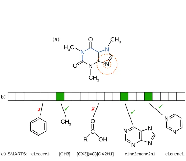
molecule. This is not a bijective relationship, meaning that different molecules can have the same fingerprint. For this reason, a molecule cannot be reconstructed from its fingerprint. Substructure properties can be described by SMARTS patterns.

One reason for the popularity of molecular fingerprints is that they allow for an efficient way to compare structures. This is of particular interest in virtual screening where one or multiple query molecules are searched against a database of millions of molecular structures [221]. The screening usually selects a small subset of candidates for further analysis. This can be either additional computational analysis, such as substructure search or the calculation of the largest common substructure shared between molecules. Especially the second task is too complex to be performed on the whole database [168]. But also additional analytical analysis, such as assays to test bioactivity, are too expensive and time-consuming to be applied to all available molecules.

The classification of molecular structures which exhibit similar biological effects or physicochemical properties, has been widely adopted in drug discovery [13]. In ligand-based screening, a structure database is searched for molecular structures similar to a molecule with known bioactivity, in order to select a set of molecules which is enriched for this desired activity [128]. This is based on the assumption of the similar properties principles: molecules with similar structures are likely to have similar properties [26, 96, 100, 219]. Quantitative structure–activity relationship (QSAR) modeling is used to directly predict biochemical properties based on the molecular structure. Early works have been reported since the 1970s [1, 222]. For an overview on QSAR modeling see Dudeket al. [59].

A widely adopted function to compare molecular fingerprints is theTanimoto coefficient

(also known as Jaccard index) [220]:

T animoto(A, B) =|A∩B|

|A∪B|,

where A and B are the sets of substructures present in the fingerprints of two molecules. Other measures are the cosine similarity and Dice coefficient, which often perform similarly in ranking tasks [7]. For comparisons of different similarity measures see Bajusz et al. [7]

(20)

Many different types of fingerprints exist, most of which are based on substructures without stereochemical information (2D fingerprints). Numerous types are implemented in popular chemistry software toolkits, such as CDK [194, 223], OpenBabel [152] and RDKit2_,

or specialized libraries [88]. There are fingerprints which consist of a fixed (sometimes hand-curated) set of structure properties. This includes PubChem CACTVS [212], MACCS and Klekota-Roth [106] fingerprints. In contrast, combinatorial fingerprints define how

to systematically generate substructure properties. The generated substructures differ based on the underlying set of molecules. The number of potential substructures of a fingerprint can be infinite. Representative combinatorial fingerprints are path and shortest path fingerprints, which enumerate all possible (shortest) paths between pairs of atoms in a molecule [88, 219]. Circular fingerprints such as the extended connectivity fingerprints (ECFP) [173] define and enumerate substructures based on atoms and their proximity. A parameter specifies the “radius”. Small substructures can be generated by considering each atom and its connected neighbors. A larger radius includes also the neighbors’ neighbors. This is an iterative approach and each iteration considers a further range of neighbors. See Fig. 2.2 for an illustration of a fingerprint. For a comparison of different fingerprint types see Benderet al. [14], Duanet al. [58], Willett and Winterman [222] and O’Boyle and Sayle

[151].

In the means of making virtual screening more efficient, “folded” fingerprints where introduced [80]. Here, the set of all molecular properties are hashed onto a fixed-size bit vector with usually 1024 or 2048 bits. As a consequence, unrelated substructures are encoded by the same position in the fingerprint vector. This may be appropriate if the workflow performance is not overly afflicted by false positive hits. But one should refrain from using these fingerprints to train machine learning models for QSAR. Folding introduces “collisions”: different molecular properties are assigned to the same fingerprint position. An “active” position in one fingerprint vector might correspond to a completely different property than in another fingerprint vector. Because of this, fingerprint positions become harder to interpret; predictive models may perform worse.

2.3 Mass Spectrometry

Mass spectrometry (MS) is one predominant technique to measure small molecules. It can measure many different molecules at the same time which enables high-throughput analysis. Furthermore, it is high-sensitive — orders of magnitude more sensitive than nuclear magnetic resonance (NMR).

In order to measure a molecule it needs to be ionized first. Mass spectrometers measure the mass-to-charge ratio (m/z) of ionized molecules. Ions can be multiple charged. A

single charged ion with a weight of 100Dahas the samem/z as a double charged ion with

a weight of 200 Da. Throughout this thesis we will assume that ions are single charged.

This is usually true for most small molecules. Hence, the m/z can be interpreted as the

mass of a molecule. Multiple charged molecules can be easily recognized by their isotope pattern (Section 4.2.1) and removed from the data. Depending on the context, we will refer to the measured ions as molecule, ion or compound. Mass spectrometry does not measure single molecules, but a signal produced by many ions of the same molecular entity.

The output of mass spectrometry is a mass spectrum: a two dimensional plot reporting ion signal intensity as a function ofm/z. The signal of a molecule is called peak. Important

2

(21)

2.3 Mass Spectrometry 11

N











CH

₃ (c) SMARTS: c1ccccc1 [CH3] [CX3](=O)[OX2H1] c1nc2cncnc2n1 c1cncnc1 (b) (a)

C

O

R

OH

O

N

O

H

₃

C

CH

₃

CH

₃

Figure 2.2: Molecular structure of caffeine and fingerprint representations. (a) Molecular structure with highlighted examples of combinatorial fingerprints. (b) Illustration of a fixed-size fingerprint with a set of substructures that are contained / not contained in caffeine. The pyrimidine ring property (rightmost illustrated structure) is a substructure of the heterocyclic purine to its left; every structure containing purine must also contain a pyrimidine ring. The SMARTS patterns in (c) can be used to match the substructures. Examples of a path (blue) and the proximity of an atom (orange circles) are indicated in (a) as representatives of all possible substructures of path fingerprints and ECFPs, respectively. Combinatorial fingerprints can be used to generate fixed-size fingerprints given a training dataset of molecules.

(22)

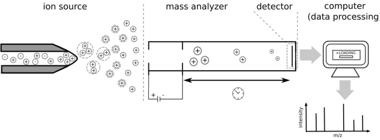
ion source mass analyzer detector computer (data processing) + -+ + + + + ++ + + + + + + + - + -+ + + + + + + + + + + + + + + ₊ + + + + + + >LOADING m/z intensity

Figure 2.3: Schematic illustration of a mass spectrometer with electrospray ionization (ESI) as ion source and a time-of-flight (TOF) mass analyzer. The mass spectrometer consists of three basic parts. From left to right: the ion source produces charged molecules. These are separated in the field-free drift region of the TOF analyzer and measured by the detector. The signal is converted into a mass spectrum. Further data processing steps may follow (Section 4.1).

instrumental parameters are mass accuracy and resolution. The mass accuracy indicates how precisely the mass of a molecule can be measured: it is the ratio ofm/z measurement

error to truem/z and is specified in parts per million (ppm). High-accuracy instruments

have mass errors below 20 ppm. The resolution specifies the ability to distinguish two peaks of highly similarm/z. One measure to specify resolution is them/z divided by the closest

distance∆m/zof two peaks of equal height that are still clearly distinguishable [138]. High resolution is important for high accuracy since it limits errors resulting from overlapping signal peaks. Signal intensity can be interpreted as a function of molecule abundance. But the relation is very complex and depends on the ionization efficiency of the molecule and also ion suppression between different molecules. Thus, it is non-trivial to infer abundance from intensity.

Functional principles Conceptionally, a mass spectrometer consists of three components

(Fig. 2.3): Theion source which ionizes the molecule, themass analyzer which separates

the molecules according to their m/z and the mass detector which detects the ions and

records signal intensity. Different types of ion sources, mass analyzers and detectors exist. Ion sources can be categorized intosoft andhard ionization sources. The first technique

only ionizes the molecule, the second additionally fragments it. A popular hard ionization technique is electron ionization (EI) [229]. Here, a beam of energetic electrons interacts

with the molecule. The fragmentation is highly-reproducible and well understood [69]. However, it is often difficult to determine them/z of the unfragmented molecular ion. EI

is frequently used in combination with a separation technique called gas chromatography (Section 2.5). A common soft ionization technique is electrospray ionization (ESI). Here,

a liquid solvent containing the analyte is pressed through a tiny capillary held at a high electric potential. The molecules form small, charged droplets. The solvent evaporates, the droplets become smaller and the charged analyte molecules repel each other to eventually break up the droplets.

(23)

2.4 Tandem Mass Spectrometry 13

A mass analyzer separates the ionized molecules according to their m/z. The mass

analyzer greatly determines the quality of the data, that is, the mass accuracy, sensitivity and resolution. In a time-of-flight (TOF) analyzer all ions are accelerated through the same electric potential by an electric field. Molecules with the same charge receive the same kinetic energy. Molecules with higher mass need more energy to accelerate, thus velocities depend on the ions’ m/z. After acceleration ions travel trough a field-free drift

region. Travel time is proportional to the square root of m/z which separates ions of

differentm/z before they reach the detector. Time-of-flight instruments are comparatively

simple in design and achieve high acquisition rates [71]. They can have high mass accuracy and resolution.

Other instruments, such as Fourier-transform ion cyclotron resonance (FTICR) MS instruments or Orbitrap, follow a quite different design principle. Here, mass analyzer and detector are not separated. Ions are trapped by an electric or magnetic field. In FTICR-MS aPenning traptraps the ions and an oscillating electric field excites them to a

larger cyclotron radius. The ions’m/z is inversely proportional to the cyclotron frequency.

The Orbitrap traps ions cycling around an electrode. Both instruments rely on the Fourier Transform to translate the ions’ frequencies into m/z values. FTICR-MS instruments

have very high mass accuracy and resolution; they can reach below1ppm mass error [24].

Orbitraps also have high resolution and mass accuracy of around 2 to 5 ppm [24]. Both instruments measure the ions in an non-destructive manner.

Ionization mode and adducts Many mass spectrometry instruments can be operated in

either positive ionization mode to produce positively charged ion species or in negative ionization mode to produce negatively charged ion species. ESI commonly produces protonated ions ([M +H]+_{) in positive ionization mode — that is, a proton is added}

to the molecule. In negative ionization mode it frequently produces deprotonated ions

([M−H]–) — that is, the molecule loses a single proton [75]. Here, “M” represents the

neutral molecule. Apart from that, different ionic species might attach to a molecule to form an adduct ion. Common adduct ions in positive ionization mode are ammonium

adduct ions ([M+NH₄]+), sodium adduct ions ([M+Na]+), and potassium adduct ions

([M+K]+_{) [110]. Common adduct ions for negative ionization mode are chlorine adduct}

ions ([M+Cl]–_{) [233]. The ratio of different adduct ions strongly depends on the used}

ionization technique and analytical setup. For example, a high salt concentration in the sample may favor [M+Na]+ _{and [M}₊_Cl]– _{ions. In the following we will call adduct ions}

“adducts” for short.

2.4 Tandem Mass Spectrometry

In tandem mass spectrometry (MS/MS) two mass analyzers are coupled together with

a fragmentation cell in between. The first mass analyzer selects ions in a certain m/z

range. Subsequently, these ions are fragmented. And finally, the fragments are recorded by the second analyzer. The resulting tandem mass spectrum (MS/MS spectrum) provides additional information about the measured molecule. This aids the discrimination of isobaric compounds (molecules with identical nominal mass) and structural isomers. While isobaric compounds might also be distinguishable by the first level of mass spectrometry (MS1), structural isomers have the same molecular formula and need MS/MS for discrimination. Stereoisomers are usually indistinguishable by mass spectrometry.

(24)

Collision induced dissociation(CID) is a common fragmentation technique coupled with

soft ionization. Here, the ions pass through a collision cell containing a collision gas. On their trajectory the ions collide with the gas which converts some kinetic energy into internal energy. This triggers a chemical reaction and the ions get fragmented into two (or more) pieces and the charge is passed on to one of the pieces. The ion that is being fragmented is called theprecursor ion; the fragmented part that carries a charge is called

product ion orfragment; and the neutral part is calledloss. Only the ionized fragments can

be measured by the subsequent mass analyzer; this produces the MS/MS spectrum. Since not only a single ion but many identical ions of the same molecular entity are fragmented at once, many fragments are recorded. Consequently, the same substructure can be both, fragment and loss. The velocity at which ions pass through the collision cell can be regulated; this changes the transferred collision energy. Higher collision energies result

in smaller fragments, whereas lower collision energies may leave ions unfragmented. To obtain a higher number of different fragments, multiple MS/MS scans may be measured at different collision energies and combined.

2.5 Chromatography

Biological samples are usually too complex to be measured directly by mass spectrometry. Highly abundant ions would interfere too much with the detection of less abundant ions. Furthermore, tandem mass spectrometry would not be able to select single ion species but mixtures for MS/MS. This makes the interpretation of MS/MS spectra challenging. Thus, mass spectrometry is often coupled to a prior separation step. Chromatography

is a technique for the separation of a mixture of different molecules based on their chemical or physical properties. The chromatography system consist of a stationary phase and amobile phase. The mobile phase carries analyte molecules through a column

containing the stationary phase. Molecules bind to the stationary phase with different affinities. Thus, different molecules pass through the column at different speeds and separate. Chromatography can be coupled with ion-mobility spectrometry to enhance separation [132].

The most prominent chromatography techniques coupled with mass spectrometry are

gas chromatography (GC) and liquid chromatography (LC). Gas chromatography-mass spectrometry (GC-MS) has been around for many decades and often uses EI as ion

source [68]. Molecules have to be — or made be — volatile. Due to the high temperatures necessary for GC, this is not applicable for larger molecules, such as peptides, which would denature. Liquid chromatography-mass spectrometry (LC-MS) based metabolomics often

uses ESI as ion source. LC can be performed with a diverse set of molecules, including many secondary metabolites [67]. Even with LC separation tens to hundred of different molecules can elute at the same time [158].

In untargeted mass spectrometry experiments, first an MS1 scan is performed to detect them/z values of all currently eluting molecules. Now, one or more high-intensity peaks

are individually selected and MS/MS scans are performed. This is done in an alternating fashion to cover the whole LC-MS/MS run with MS1 and MS/MS spectra. Still, many compounds might not be covered by MS/MS. The time at which a molecule elutes is called theretention time. This can be used as orthogonal information, in addition to a molecule’s m/z and MS/MS spectrum, to assist identification. Whereas GC retention times can

(25)

2.5 Chromatography 15

systems produce retention times with much greater variation [227]. The LC retention time of a molecule differs between setups and can even change from run to run on the very same instrument. Nevertheless, retention times can be utilized as orthogonal information to confirm the identity of a compound: A known reference compound can be spiked into the sample to check if it elutes at the same retention time as the unknown compound of interest.

(26)

(27)

3 Statistics and Graph Theory

In this chapter, we provide graph-theoretical notations and definitions. Then, we give a short introduction to Bayesian statistics and Bayesian inference. We refer readers who are less familiar with graph theory to one of the many graph theory textbooks such as Diestel [54]. For a more comprehensive view on Bayesian statistics in general see Koch [107] and Liu [120] for Monte Carlo methods in particular.

3.1 Graph Theory

Graphs are a mathematical concept to model pairwise relations between objects. Here, we introduce the basic terminology from graph theory.

A graph G = (V, E) consists of a set of nodes V and a set of edges E. Edges depict relations between nodes; each edge connects two nodes. Graphs can be either directed or undirected. In undirected graphs, edges are unordered pairs of nodesE ⊆(︁V

2

)︁

, where (︁V

2

)︁

is the set of all two-element subsets ofV. Directed edges are two-element tuples (u, v) of

nodesu, v∈V. Thus, for directed graphs the edge set is E ⊆V ×V. Two nodesu, v∈V areadjacent to each other if they are connected by an edge. Apath is a sequence of edges

such that consecutive edges share exactly one node and each edge is used at most once; in directed graphs, the ending node of one edge must be the starting node of the next edge in the sequence. A path with the same node as start and endpoint is calledcycle. A directed

graph that does not contain any cycle is calleddirected acyclic graph (DAG). For a directed

edge(u, v) ∈E in a DAG we callu theparent and v thechild. A tree T = (V, E) is an

undirected graph in which any two nodes are connected by exactly one path. A rooted tree has a designated vertex r called root. All directed edges point away from this root. A graphG′ = (V′, E′) is a subgraph of G if and only if V′ ⊆V and E′ ⊆E. A clique in

an undirected graph G is a subset of nodes S ⊆ V, such that every two nodes in S are connected by an edge inG.

Graphs can be colored and labeled to categorize nodes or edges, or to assign them a certain feature. In fragmentation graphs and fragmentation trees, which are introduced in Section 4.2.2, the nodes and edges are labeled with molecular formulas in order to explain fragments and losses in a spectrum. Colors are usually introduced to assign nodes to a common origin. Different nodes with the same color can correspond to different hypotheses assigned to the same origin. A graph is colorful if every node has an unique color. This

allows to formulate optimization problems which decide between different hypotheses by finding an optimal colorful subgraph. For example, a peak in a mass spectrum could be explained by multiple molecular formula candidates. Here, the candidates are nodes and the peak is represented by a color. When selecting a colorful subgraph, only one valid candidate may be retained.

Nodes and edges can be weighted to associate some measure of cost or importance. Edge-weighted graphs have ascoring function wE :E →R. Analogously, vertex-weighted

graphs have a scoring functionwV :V →R.

(28)

3.2 Bayesian Statistics

Bayesian statistics is a fundamental theory in the field of statistics in which probability quantifies the belief in a hypothesis or the certainty of an event. Probabilities do not have to be based solely on observations. Instead, Bayesian statistics allows to incorporate prior information and express this in form of probabilities. This prior information can be derived from many different sources. It may be expert knowledge: here, the probabilities express a measure of plausibility that a hypothesis is indeed true. It may also be a summary of prior experimental results, or a hypothesized generic distribution over events in the sample space.

Suppose we want to estimate the distribution of body heights of people in, say, Germany. The distribution of body heights of the general world population offers a good estimate of body heights in Germany. This prior knowledge tells us that adult humans rarely have heights below 1 or above 2.5 meters. If we do not have any data specifically for Germany, then this is a good estimate. We could now conduct an experiment and measure people from Germany. If we select two random German people and measure their heights, this will give a bad approximation of German body height distribution. Hence, the world-wide population is still the better estimate. However, if we measure 100,000 German people, we may end up with an even better estimate. Now, at what number do we trust our sample statistic more than the prior information? After 10 samples? Or after 100 samples? With Bayesian statistics we do not have to decide for an arbitrary threshold. Rather, it enables us to combine the prior knowledge with the data, thus making best use of all available information.

Let us define this more formally: Given are the data D (our samples), and we want to

estimate the unobserved model parametersM. Then, theprior probability is a probability

distribution P(M) over all possible model parameters. The likelihood P(D|M) is the conditional probability that our sample data was produced under the given parameter set. This enables us to calculate aposterior probability _P(M|D) using Bayes’ theorem:

P(M|D) = P(

D|M)P(M)

P(D) . (3.1)

Now, back to our example. Assume that body heights are normally distributed and we observed body heights of German people D ∈ D. The unobserved parameters of our

model are the meanµ and standard deviation σ of normal distribution N(µ, σ2). Given

a sample statistic of the world population, we can estimate prior probabilities of these parameters — this isP(M). Furthermore, we can calculate how likely specific parameters would generate the data D — this is P(D|M). When we combine all this information, we can estimate the model parameters. Finding the most probable model parameters based onP(M|D) corresponds to a maximum a posteriori (MAP) estimate. If we do not have any prior knowledge of the model parameters M, we usually assume a flat prior

— all parameter realizations are equally probable. This results in a maximum likelihood (ML) estimate: the model which most likely generates the data is the most likely model. To calculate P(D), we would need to marginalize over all possible parameter realizations ofM. However, this is not necessary in order to find the most probable parameters based

on P(M|D). The denominator in equation (3.1) is the same for all model parameters. SinceP(M|D)∝P(D|M)P(M) we can ignoreP(D) and only maximizeP(D|M)P(M).

(29)

3.3 Bayesian Inference 19

3.3 Bayesian Inference

Bayesian inference is a method to infer the probability of a hypothesis using the Bayes’ theorem. This can be as simple as weighing the hypothesis “the die is fair” against “the die is biased”. But it can also be used to assign posterior probabilities to all possible parameter realizations of a highly-dimensional model. ML or MAP estimation essentially become optimization problems that predict a single point in parameter space. However, this is not appropriate for all applications. Especially, if the posterior probability is not a regular unimodal distribution with most probability being “concentrated” in one high peak. Here, Bayesian inference can help and estimate the whole posterior probability distribution. For example, assume a game of dice is played, but the casino frequently switches between fair and biased dice. Thus, both models, “dice are fair” and “dice are biased”, are true and coexist with different probabilities. Another example is about risk assessment: based on the weather forecast, we predict if the wind will become a hurricane in the coming days. The MAP estimation might predict wind speeds of exactly39 km/h. Using Bayesian

inference we might come to the conclusion that there is still a 20 % chance that wind speeds will exceed120 km/h. Both statements are correct. However, Bayesian inference provides

the more relevant information in this example. This illustrates the inherent difference between these methods. There also exists a range of approaches in between single-point estimates and the calculation of the whole posterior probability distribution which are not covered in this thesis.

The posterior probability distribution can often not be solved analytically. Monte Carlo methods can be used to generate a representative sample of the underlying distribution. From this, the distribution can be approximated and statistics can be derived. Monte Carlo sampling was initially used to solve physics-related problems [130]. Nowadays many applications for statistical inference are based on the concept.

What does “sampling from a probability distribution” imply formally? Conducting a random experiment results in a single outcome from a set of possible outcomes. Random variables are functions that map outcomes to some measurable space. In this way they

group possible outcomes toeventsand give them some meaning. A probability distribution

assigns probabilities to the possible events of a random variable. Take for example a six-sided die. Rolling the die will result in one out of six possible outcomes of 1,2,3,4,5

and 6. A random variable X may divide outcomes into the two events x0 = “the number of pips is even” and x1 = “the number of pips is odd”. This can be defined by the mapping {2,4,6} → x0 and {1,3,5} → x1. In the discrete case the probability distribution can be described by aprobability mass function p: pX(x0) =P(X=x0) = 1/2

and pX(x1) =P(X =x1) = 1/2. We may refer to pX as p for short if it is obvious which

random variable is considered. Continuous random variables that map outcomes to an uncountable infinite number of events can be described by probability density functions

instead. Sampling a random variable X yields a realization x, that is, an event of the random variable chosen according toP(X).

Generating independent samples from a target probability distribution p(x) in such a

way to closely resemble the underlying distribution is often infeasible. This is especially the case for high-dimensional parameter spaces, where most parameter realizations have very low — close to zero — probability and do not considerably contribute to the probability distribution. Importance sampling was suggested to sample from a different

(30)

is meaningful non-zero [127]. Alternatively, Markov chain Monte Carlo (MCMC) can be

used to generate a sequence of random samples. All MCMC methods are governed by theMarkov property which states that the probability of each event only depends on the

state of its preceding event; all previous states are irrelevant. For a sequence of random variablesX(1), X(2), . . . , X(t+1)and corresponding realizationsx(1), x(2), . . . , x(t+1)this can be formalized as:

P(X(t+1)=x(t+1)|X(t) =x(t), X(t−1) =x(t−1), . . . , X(1)=x(1))

=P(X(t+1)=x(t+1)|X(t) =x(t)).

A stochastic process that satisfies this property is calledMarkov chain (or Markov process

in the continuous case). It is uniquely described by itstransition function T(x, x′) which

defines the probability of transitioning from one statexto any other statex′. A distribution p(x) is said to be invariant with respect to the Markov chain if the transition function

leavesp(x) unchanged:

p(x′) =∑︂ x

T(x, x′)p(x). (3.2) Two properties are commonly desired for a given Markov chain:

1. irreducibility: A chain is irreducible if it is possible to get from any state to any other state (not necessarily in one step).

2. aperiodicity: A state x is k-periodic if every sequence of states which starts with x and ends inx has a number of steps which is a multiple ofk. If k= 1, then the state

x is aperiodic, otherwise it is periodic. A Markov chain is aperiodic if every state is aperiodic.

If a Markov chain is irreducible and aperiodic, then the chain will becomestationary at a

unique invariant distribution. Various algorithms exist for constructing Markov chains, most notably the Metropolis-Hasting algorithm [82]. MCMC methods are frequently applied to bioinformatics problems [92]. Popular applications include sequence-based approaches such as finding DNA binding motifs [116] and phylogenetic inference [230].

3.4 Gibbs Sampling

Gibbs sampling is a suitable MCMC method if the conditional distributions of the variables are known and easy to sample from. Gibbs sampling, in its basic version, is a special case of the Metropolis-Hastings algorithm [82, 131]. Metropolis-Hastings in general defines transition probabilities based on a proposal functiong(x′|x)and an acceptance probability

A(x, x′). The proposal function generates a new state based on the current one. Then,

this new state is accepted proportional to the acceptance probability; if it is rejected, the state remains unchanged. Recall, that in order to generate samples from the target distributionp(x), the distribution needs to be invariant to the transition functionT(x, x′).

The proposal function does not ensure appropriate transition probabilities. Rather, the acceptance probabilities are chosen, such that the combination of proposal and acceptance probabilities results in the desired transition probability. Thus, the actual transition function is T(x, x′) = g(x′|x)A(x, x′). However, poorly chosen proposal functions may