Adaptive Approximations for
High-Dimensional Uncertainty
Quantification in Stochastic
Parametric Electromagnetic
Field Simulations
Zur Erlangung des akademischen Grades Doktor-Ingenieur (Dr.-Ing.) genehmigte Dissertation vonDimitrios Loukrezis aus Athen, Griechenland Tag der Einreichung: 29. October 2018, Tag der Prüfung: 04. February 2019 Darmstadt — D 17
1. Gutachten: Prof. Dr.-Ing. Herbert De Gersem 2. Gutachten: Prof. Dr.-Ing. Ulrich Römer
Fachbereich Elektrotechnik und Informationstechnik Institut für Theorie Elektromagnetischer Felder
Adaptive Approximations for High-Dimensional Uncertainty Quantification in Stochastic Parametric Electromagnetic Field Simulations
Genehmigte Dissertation vonDimitrios Loukrezis aus Athen, Griechenland 1. Gutachten: Prof. Dr.-Ing. Herbert De Gersem
2. Gutachten: Prof. Dr.-Ing. Ulrich Römer Tag der Einreichung: 29. October 2018 Tag der Prüfung: 04. February 2019 Darmstadt — D 17
Bitte zitieren Sie dieses Dokument als:
URN: urn:nbn:de:tuda-tuprints-84854
URL: http://tuprints.ulb.tu-darmstadt.de/84854
Dieses Dokument wird bereitgestellt von tuprints, E-Publishing-Service der TU Darmstadt
http://tuprints.ulb.tu-darmstadt.de [email protected]
Die Veröffentlichung steht unter folgender Creative Commons Lizenz:
Namensnennung – Keine kommerzielle Nutzung – Keine Bearbeitung 4.0 Interna-tional
Erklärung zur Dissertation
Hiermit versichere ich, die vorliegende Dissertation ohne Hilfe Dritter
nur mit den angegebenen Quellen und Hilfsmitteln angefertigt zu
haben. Alle Stellen, die aus Quellen entnommen wurden, sind als
solche kenntlich gemacht. Diese Arbeit hat in gleicher oder ähnlicher
Form noch keiner Prüfungsbehörde vorgelegen.
Darmstadt, den 04. February 2019
Contents 1 Introduction 1 1.1 Motivation . . . 1 1.2 Contribution . . . 4 1.3 Structure . . . 4 2 Preliminaries 6 2.1 Stochastic Parametric Models . . . 6
2.1.1 Model Problem: Dielectric Slab Waveguide with Random In-puts . . . 8
2.2 Uncertainty Propagation and Quantification . . . 12
2.3 Spectral Methods for Uncertainty Quantification . . . 16
2.4 Downward-Closed Multi-Index Sets . . . 17
2.5 Adaptivity . . . 18
2.6 Concluding Remarks . . . 19
3 Dimension-Adaptive Stochastic Collocation 20 3.1 Stochastic Collocation . . . 20
3.1.1 Univariate Stochastic Collocation . . . 21
3.1.2 Tensor-Product Stochastic Collocation . . . 22
3.1.3 Stochastic Collocation on Smolyak Sparse Grids . . . 23
3.2 Nested Nodes and Hierarchical Interpolation . . . 25
3.3 Dimension-Adaptive Stochastic Collocation . . . 28
3.4 Nested Collocation Points . . . 29
3.4.1 Leja . . . 29
3.4.2 Clenshaw-Curtis . . . 31
3.5 Post-processing the Approximation . . . 32
3.6 Application to the Model Problem . . . 34
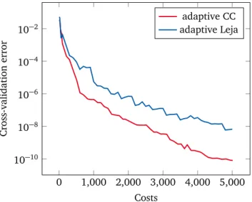
3.6.1 Leja versus Clenshaw-Curtis for Uniform Input Distributions . 36 3.6.2 Leja versus Clenshaw-Curtis for Non-Symmetric Beta Input Distributions . . . 40
3.7 Concluding Remarks . . . 41
4 Basis and Sampling-Adaptive Generalized Polynomial Chaos 43 4.1 Generalized Polynomial Chaos . . . 43
4.1.1 Univariate Polynomial Chaos Expansions . . . 44
4.1.2 Multivariate Polynomial Chaos Expansions . . . 44
4.2 Adaptive Polynomial Chaos Expansions . . . 49
4.2.1 Basis Adaptivity . . . 49
4.2.2 Sampling Adaptivity . . . 52
4.3 Post-processing the Approximation . . . 54
4.4 Application to the Model Problem . . . 56
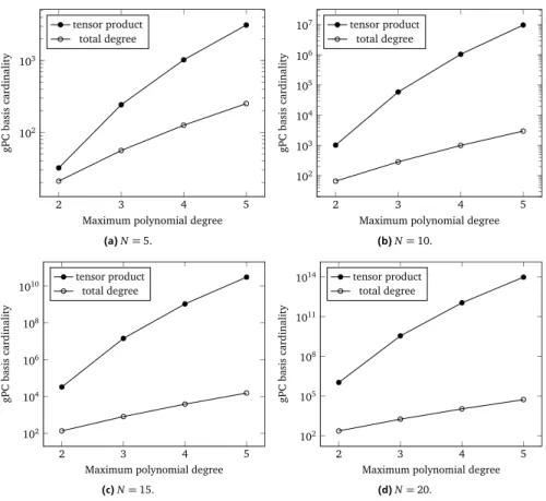
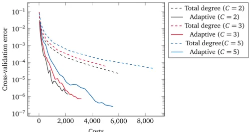
4.4.1 Adaptive versus Total Degree gPC Bases . . . 57
4.4.2 All-In versus One-to-One Basis Adaptivity . . . 60
4.4.3 Random versus Quasi-Random Experimental Designs . . . 60
4.4.4 Basis/Sampling Adaptivity versus Basis Adaptivity . . . 62
4.4.5 Basis/Sampling Adaptivity versus Least Angle Regression . . . 63
4.5 Concluding Remarks . . . 64
5 Low-Rank Tensor Decompositions 65 5.1 Basics of Multi-Linear Algebra . . . 65
5.2 Tensor Decompositions . . . 68
5.2.1 The Two-Dimensional Case . . . 68
5.2.2 Canonical Polyadic Decomposition . . . 70
5.2.3 Tucker Decomposition . . . 71
5.2.4 Tensor-Train Decomposition . . . 72
5.3 Uncertainty Quantification with Tensor Decompositions . . . 73
5.4 Application to the Model Problem . . . 74
5.5 Concluding Remarks . . . 76
6 High-Dimensional Numerical Experiments 78 6.1 Cole-Cole Permittivity . . . 78 6.1.1 Model . . . 79 6.1.2 Numerical Results . . . 80 6.2 Stern-Gerlach Magnet . . . 85 6.2.1 Model . . . 85 6.2.2 Numerical Results . . . 88
6.3 Resonant Cavity Filter . . . 91
6.3.1 Model . . . 92
6.3.2 Numerical Results . . . 95
6.4 Concluding Remarks . . . 97
7 Conclusion and Outlook 99 7.1 Conclusion . . . 99
7.2 Outlook . . . 100
Abstract
The present work addresses the problems of high-dimensional approximation and uncertainty quantification in the context of electromagnetic field simulations. Such problems are typically encountered during the design phase of electromag-netic devices, e.g. magnets or high-frequency components. Manufacturing toler-ances, material contaminations, or other types of imperfections introduce, possibly many, sources of uncertainty with respect to the device’s characteristics, e.g. ge-ometry, material properties, or operational data, which in turn affect the overall operation of the device. For the final designs to be robust and the manufactured device to operate within its specifications, this uncertainty must be accounted for in the simulation-based studies performed during the design phase.
In the presence of many parameters, one faces the so-called curse of dimensional-ity, i.e. the computational complexity increases exponentially as the number of pa-rameters, equivalently, dimensions, grows. The focus of this work lies on adaptive methods that mitigate the effect of the curse of dimensionality, and therefore en-able otherwise intracten-able uncertainty quantification studies. Its application scope includes electromagnetic field models suffering from moderately high-dimensional input uncertainty. However, the presented methods can be used in a black-box fash-ion and are therefore applicable to other types of problems as well, such as fluid dynamics or structural mechanics, provided that the underlying assumptions, e.g. smoothness, are satisfied. To that end, three different approaches are investigated. The first approach relies on a dimension-adaptive stochastic collocation scheme. Emphasis is placed on the use of the commonly employed Clenshaw-Curtis collo-cation points and the relatively recently investigated Leja collocollo-cation points, for both uniform and non-uniform input distributions. It is shown that combining the stochastic collocation method with a well-known dimension-adaptive algorithm results in significant computational savings compared to the isotropic collocation variant. For the case of uniformly distributed input parameters, the performance of Leja nodes is found to be advantageous in terms of approximation accuracy, but in-ferior for quadrature purposes, compared to Clenshaw-Curtis nodes. The reverse is observed for the case of skewed beta input distributions, where Leja nodes yield in-ferior approximation accuracies, but offer significant advantages in the quadrature context.
The second approach employs adaptively constructed generalized polynomial chaos expansions. A two-level adaptivity is considered. The first adaptivity level refers to the construction of the polynomial basis given an experimental design of fixed size. The second adaptivity level refers to the adaptive expansion of the experimental design, whenever necessary due to numerical stability requirements. We note that a drawback of this second level of adaptivity is its dependence on an
a priori set limit value κmax regarding the condition number of a system matrix, which acts as a stability indicator. Based on this two-level adaptivity approach, an in-house algorithm has been developed in the course of this work. The algorithm is presented in detail and tested against isotropic polynomial chaos expansions, showing significant computational savings. The algorithm is also compared against a state-of-the-art adaptive polynomial chaos approach and is found to be superior, even for conservative, pessimistic values ofκmax.
The third approach is based on low-rank tensor decompositions. Exploiting the underlying tensor structure of the multivariate quadrature formulas which are em-ployed for the numerical computation of statistical moments, tensor decomposi-tions are employed to reduce the complexity of the multi-dimensional arrays, i.e. tensors. First, it is shown how quadrature weight tensors may admit exact low-rank representations. Next, high-order adaptive cross approximation methods are used to compute low-rank approximations of the function-generated tensors which con-tain the model evaluations on the quadrature nodes. The resulting low-rank tensor decompositions are then used for the estimation of statistical moments at a reduced cost. The numerical results show that the approach yields tremendous complexity reductions compared to full tensor-product quadratures, however, it is significantly more expensive compared to the aforementioned collocation and polynomial chaos approaches.
The implementations of all considered approaches are documented in in-house developed Python and MATLAB scripts and software libraries. Extensive numerical tests are presented for all methods with respect to their accuracy and computational cost. The methods are tested on simulation models of both toy examples and real-world electromagnetic field applications, featuring a moderately high number of uncertain parameters.
Kurzfassung
Die vorliegende Arbeit befasst sich mit hochdimensionaler Approximation und Unsicherheitsquantifizierung im Kontext elektromagnetischer Feldsimulation. Solche Probleme treten typischerweise während der Entwurfsphase eines elektro-magnetischen Geräts auf, z.B. eines Magneten oder einer Hochfrequenzkompo-nente. Herstellungstoleranzen, Materialkontamination oder andere Mängel stellen Unsicherheitsquellen in Bezug auf die Eigenschaften des Gerätes dar, die dessen Be-dienung beeinflussen können. Um eine robuste und zuverlässige Funktionsweise, am Ende des Entwurfsprozesses sicherszustellen, müssen Unsicherheiten in simu-lationsbasierten Analysen, die während der Entwurfsphase durchgeführt werden, berücksichtigt werden.
Wenn Unsicherheiten in vielen Eingangsparametern vorliegen, tritt der sogenan-nte Fluch der Dimensionalität auf, d.h. die Komplexität steigt exponentiell mit der Anzahl von Parametern. Der Schwerpunkt dieser Arbeit liegt auf der Ver-wendung von adaptiven Methoden, die den Effekt des Fluches der Dimensional-ität abschwächen und daher aufwendige Unsicherheitsquantifizierungsstudien er-möglichen. Der Anwendungsbereich umfasst elektromagnetische Feldmodelle, die eine moderat hochdimensionale Eingangsunsicherheit aufweisen. Die vorgestell-ten Verfahren sind jedoch auch auf andere Arvorgestell-ten von Problemen anwendbar, z.B. aus den Bereichen der Fluiddynamik oder Strukturmechanik. Zu diesem Zweck werden drei verschiedene Ansätze untersucht.
Der erste Ansatz basiert auf einer dimensionsadaptiven stochastischen Kolloka-tionsmethode. Der Schwerpunkt liegt auf der Verwendung von Leja und Clenshaw-Curtis Kollokationspunkten für gleichverteilte und nicht gleichverteilte Zufallsvari-abeln. Es wird gezeigt, dass die Kombination der stochastischen Kollokations-methode mit einem bekannten dimensionsadaptiven Algorithmus zu signifikan-ten rechnerischen Einsparungen im Vergleich zur isotropen Kollokationsvariante führt. Für den Fall gleichverteilter Parameter haben sich Leja-Knoten im Ver-gleich zu Clenshaw-Curtis-Knoten, im Hinblick auf die Genauigkeit der Approx-imation, als vorteilhaft erwiesen, für Quadraturzwecke jedoch als unterlegen. Das Umgekehrte wird für den Fall von nicht-symmetrischen Betaverteilungen beobachtet, wo Leja-Knoten geringere Approximationsgenauigkeiten ergeben, je-doch signifikante Vorteile im Quadraturkontext bieten.
Der zweite Ansatz verwendet adaptive generalisierte Polynomiale-Chaos En-twicklungen. Dabei wird eine zweistufige Adaptivität verwendet. Die erste Adaptiv-itätsstufe bezieht sich auf die Konstruktion der Polynombasis bei einer Versuchspla-nung fester Größe. Die zweite Adaptivitätsstufe bezieht sich auf die adaptive Er-weiterung der Versuchsplanung, aufgrund numerischer Stabilitätsanforderungen. Basierend auf diesem zweistufigen Adaptivitätsansatz wurde im Rahmen dieser
Arbeit ein Algorithmus entwickelt. Der Algorithmus wird im Detail vorgestellt und gegen isotrope polynomiale Chaosexpansionen getestet, wobei signifikante Einsparungen bei der Rechenzeit erzielt werden. Der Algorithmus wird darüber hinaus auch mit einem state-of-the-art Polynomialen-Chaos-Ansatz verglichen, dem gegenüber er überlegen ist.
Der dritte Ansatz basiert auf Niedrigrang-Tensorzerlegungen. Dazu wird die zu-grundeliegende Tensorstruktur von multivariaten Quadraturformeln genutzt, die für die numerische Berechnung statistischer Momente verwendet werden. Ten-sorzerlegungen werden angewandt, um die Komplexität der mehrdimensionalen Arrays, d.h. Tensoren, zu reduzieren. Zuerst wird gezeigt, wie Tensoren bestehend aus Quadraturgewichten eine exakte Niedrigrang-Darstellung zulassen. Als Näch-stes werden adaptive Kreuznäherungsverfahren höherer Ordnung angewandt, um die funktionserzeugten Tensoren in einem Niedrigrang-Format zu approximieren, die die Modellauswertungen auf den Quadraturknoten enthalten. Die resultieren-den Niedrigrang-Tensorzerlegungen werresultieren-den dann für die Schätzung von statistis-chen Momenten verwendet. Es wird gezeigt, dass dieser Ansatz im Vergleich zu vollständigen Tensor-Produkt-Quadraturen zu enormen Komplexitätsreduktionen führt. Der Ansatz ist jedoch im Vergleich zu den oben genannten Kollokations- und Polynomialen-Chaos-Ansätzen deutlich teurer.
Die Implementierungen aller Ansätze sind in selbstentwickelten Python- und MATLAB-Skripten sowie Software-Bibliotheken dokumentiert. Umfangreiche nu-merische Tests werden für alle Methoden hinsichtlich ihrer Genauigkeit und ihres Rechenaufwandes präsentiert. Die Methoden werden an Simulationsmodellen von sowohl stark vereinfachten Simulationsmodellen als auch an realen elektromag-netischen Feldproblemen getestet, die eine moderat hohe Anzahl von unsicheren Parametern aufweisen.
1 Introduction
In this introductory chapter we present general information about the present thesis. The chapter begins with the motivation that led to this particular thesis topic. Next, we discuss the contributions of the present work withing this research field. The structure of the thesis is presented at the end of the chapter.
1.1 Motivation
Various engineering branches employ nowadays “in silico” models [68], i.e. com-puter programs or softwares which simulate physical phenomena by solving the underlying mathematical problems on a computer. Simulation-based parameter studies, such as optimization, sensitivity, or uncertainty analyses, allow for thor-ough examinations of the relations between a model’s input parameters and its output quantities. The results of such studies are often used to improve the de-signs of actual physical systems and devices, such as magnets, electrical machines, waveguides or antennas, to name a few indicative examples.
The relatively young field of uncertainty quantification (UQ) has emerged among the computational sciences to address the need of taking uncertainty into account when performing simulation-based studies. Although state-of-the-art models be-come increasingly accurate thanks to sophisticated computational methods and powerful computer hardware and software, uncertainties with respect to the model parameters gives rise to uncertainties regarding the model output quantities as well. Let us for example consider the case of designing and eventually producing an electromagnetic device. While parameter values which result in the expected operation of the device can be identified during the design phase, manufacturing or other tolerances may cause the actual values of said parameters to deviate from the desired ones. As a consequence, a suboptimal operation or, in extreme cases, even a failure of the device are possible outcomes. Therefore, uncertainty must be taken into consideration in order to minimize the risk of such events.
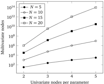
A common bottleneck in multi-parameter studies is the so-called “curse of di-mensionality”. The term is attributed to R. E. Bellman [18] and refers to a variety of difficulties which arise in computational tasks performed in high-dimensional spaces. Most commonly, the curse of dimensionality manifests in the form of paralyzing complexities which render the computational costs of standard meth-ods unaffordable. High-dimensional UQ is no stranger to such problems. For example, estimating a statistical moment of a model output typically reduces to computing a multivariate integral. As illustrated in Figure 1.1, a numerical integra-tion scheme based on tensor-product combinaintegra-tions of univariate quadrature rules becomes quickly intractable for an increasing number of parameters. Since the strength of modern simulation models lies, to a large extent, in their capability to
2 3 4 5 102 104 106 108 1010 1012 1014
Univariate nodes per parameter
Multivariate nodes N=5 N=10 N=15 N=20
Figure 1.1:Exponential complexity growth of a simple quadrature scheme withN dimensions/parameters.
incorporate a large number of parameter dependencies, the development of meth-ods which allow to mitigate or even break the curse of dimensionality is currently a very active field of research1.
Methods such as active subspaces [43] and model order reduction [35, 74] at-tempt a dimensionality reduction before proceeding to the actual parameter study. In the context of stochastic electromagnetic field (EMF) simulations, such methods have been successfully applied in [19, 79, 134], among other works. However, dimensionality reduction is not always possible and in many cases a large number of parameters must be considered as not to compromise the accuracy. The clas-sic Monte Carlo (MC) sampling approach [31, 90] is not affected by the number of parameters, however, its slow convergence rate makes the method unattractive when a high accuracy is required. An improved convergence can be achieved with quasi-MC [31, 90] and multilevel MC [62] methods, under certain assumptions.
Assuming some regularity in the model’s input-to-output map, a high-order alge-braic, or even exponential convergence can be achieved with the use of UQ meth-ods based on spectral approximations [61, 87, 162]. Spectral UQ methmeth-ods have 1 There is a certain irony here, also pointed out in [43], in the sense that increased model
com-plexity is supposed to be a means to reduce uncertainty. Instead, it often becomes a gateway to further uncertainty sources.
been applied to problems from fluid dynamics [87, 147], structural mechanics [22] and microwave engineering [5], to mention just a few application domains. The stochastic Galerkin method [8, 61, 101] is considered to be the optimal one in terms of the accuracy-cost ratio, however, the method requires a dedicated solver for each considered problem. This requirement is usually regarded as a major drawback, es-pecially in the case of complex simulation models where access “under the hood” is not provided, e.g. when a commercial software is used as a black-box. In most prac-tical applications, scientists and engineers turn to the stochastic collocation method [6], or to generalized polynomial chaos (gPC) [164] approximations based on re-gression [24, 106] or pseudo-spectral projection [49, 88]. Those approaches are preferred because they achieve accuracy-cost ratios which are comparable to the stochastic Galerkin ones, while at the same time being non-intrusive, i.e. they al-low a black-box use of the simulation model. We note that there is no universally agreed definition regarding the “intrusiveness” of a method [63], however, here we use the usual distinction.
In high dimensions, adaptive approximations are used to circumvent the curse of dimensionality. Adaptive stochastic collocation approaches have been consid-ered in [37, 60, 83, 96, 110, 117, 139]. Methods and algorithms for adaptive gPC can be found in [2, 22, 24, 102, 113]. More recently, on the basis of the observa-tion that the multivariate polynomial bases employed in spectral approximaobserva-tions have an underlying tensor structure, methods based on tensor decompositions [69, 70, 84] and low-rank tensor approximations [11, 12, 124, 137, 138, 167] have gained increasing interest. The main idea behind all adaptive methods is that, in most practical cases, the output of a model is rarely affected equally by variations from all model parameters, i.e. some parameters are more significant than others. Assuming that such a parameter anisotropy exists, adaptive methods and the corresponding algorithms are employed to separate the significant param-eter contributions from the negligible ones. The consequent anisotropic investment of computational resources results in computational savings without compromising the desired accuracy.
The focal point of the present work is to enable high-dimensional UQ in the context of EMF simulations, exactly by exploiting the aforementioned parame-ter anisotropy. We note that we focus on uncertainty propagation problems only. Other types of UQ studies, such as Bayesian parameter estimation [140] or model-form uncertainty [131], while definitely interesting, are not pursued in this work. We consider adaptive approaches for UQ purposes in the contexts of stochastic collocation, gPC and tensor decompositions. Both established methods and new algorithms, developed as part of this work, are applied to EMF simulation mod-els suffering from moderate to high-dimensional input uncertainty. While we only
consider here applications related to EMF problems, we note that the application scope of all considered approaches is vastly broader.
1.2 Contribution
As indicated by the number of already cited works, the methods which are ex-amined in the present thesis have been extensively analyzed and used in various fields and applications. We consider the main contributions of this work to be the following:
1. The implementation of a dimension-adaptive stochastic collocation algorithm and its application for uniform and fairly “exotic” input probability density functions (PDFs), in particular skewed beta ones. The latter case has not been considered in the literature so far. Moreover, the method has hardly been applied to concrete engineering applications. We have contributed in this direction with our works [57, 96].
2. The development of an algorithm for the adaptive construction of gPC ap-proximations. The adaptive expansion of both the gPC polynomial basis and the experimental design is considered. To the author’s knowledge, the pro-posed adaptive scheme is new and distinctly different from other adaptive gPC algorithms available in the literature, see e.g. [2, 22, 24, 102, 113]. 3. The application of tensor decompositions for statistical moment estimations
and their comparison against isotropic and adaptive stochastic collocation and gPC methods with respect to accuracy and computational effort. As in the collocation case, complicated engineering examples have barely been con-sidered in the literature. In the context of EMF simulations, we are aware of the work of Zhang et al. [167] and our own contribution [97].
4. The application of all aforementioned approaches to a number of EMF appli-cations, ranging from low- to high-frequency electromagnetics. Both simple toy examples and real-world models have been used for verification purposes. 5. The development of Python and MATLAB software libraries for all of the
aforementioned methods and algorithms. 1.3 Structure
The present thesis is organized as follows. Chapter 2 discusses some necessary preliminary notions which will be used throughout the thesis. The next three chap-ters present the methods and approaches which are examined in this work. In Chapter 3 we recall the basics of the stochastic collocation method and present a
hierarchical collocation scheme based on nested collocation points. Chapter 4 first presents the theory behind gPC approximations and then discusses a number of algorithms for its adaptive construction, in terms of both basis and experimental design expansion. Chapter 5 presents the notion of tensors and tensor decom-positions in the context of multi-linear algebra. Common tensor decomdecom-positions are presented, along with a discussion on their strengths and weaknesses. Em-phasis is placed on available black-box methods and algorithms for the adaptive cross approximation of tensors and their use in the context of UQ. In all three methodology-related chapters, an academic waveguide model with random input data is used to verify the advantages of the proposed adaptive methods. The penul-timate Chapter 6 presents the application of all aforementioned approaches to moderately high-dimensional stochastic parametric models. Both analytical and discretized models with 11−14uncertain parameters are considered, the latter based on the finite element method (FEM) or on isogeometric analysis (IGA). The thesis ends with a conclusion on the findings of the presented work and with a discussion on possible extensions, both available in Chapter 7.
2 Preliminaries
In this chapter, we discuss some necessary preliminaries which will be used throughout this thesis. The chapter starts by providing brief explanations of the terms “parametric” and “stochastic parametric”, which characterize the here-considered problems and models. For further clarification, a stochastic parametric EMF problem and its mathematical model are presented, namely a dielectric slab waveguide with random inputs. We proceed with the description of the objectives of uncertainty propagation and quantification. In the same section we provide the definitions of the error metrics which will be used in subsequent chapters. Next, we offer a short introduction to spectral UQ methods. The chapter continues with definitions related to the downward-closedness property of a set, which is often re-called in subsequent chapters. Finally, general notions on adaptivity are introduced, with emphasis on a posteriori error indicators.
2.1 Stochastic Parametric Models
We start by defining a mathematical model as the collection of variables and the relations among them, which are used in order to describe a phenomenon in the form of equations [68, 119]. In the context of this work, a mathematical model shall always describe a physical phenomenon, in particular related to EMFs. How-ever, the use of mathematical models extends well beyond the natural sciences. The digital form of a mathematical model, enabling the study of the underlying physical problem on a computer, will be referred to as the computational, or com-puterized, or in-silico, or simulation model [68, 119]. We distinguish between a simulation model and a simulation, such that the latter refers to a model evaluation for a specific model configuration, e.g. regarding its solver settings or input values. Evaluating a model is often encountered in the literature as “running” a simulation or “calling” a model.
In this work we employ parametrized simulation models, the predictions of which depend on a set of input parameters. We only consider parameters which affect the underlying mathematical model, e.g. the size and shape of the computa-tional domain or certain material properties. Parameters related to discretization, tolerances or other solver-specific settings of the simulation model are assumed to be chosen accurately enough for the considered application and are not considered as model input parameters. The goal of parameter studies is to use the afore-mentioned parametrized models in order to examine the relation between their input parameters and one or several model outputs, commonly referred to as the quantities of interest (QoIs).
Table 2.1:Notation summary for parametric problems.
Symbol Explanation
y∈RN N-dimensional parameter vector g:RN→R map from the input parameters to the QoI G(u(y)) =g(y) parameter-dependent QoI
Let us attempt a first formalization of the parametric problem setting. We as-sume that the physical problem at hand is tackled by solving numerically a set of parametric partial differential equations (PDEs), given in the general form
D(u,y) =0, (2.1)
whereD=D(u,y)is a differential operator,u=u(y)is the solution of (2.1) and
y∈RN is anN-dimensional parameter vector. The QoI is typically given as a func-tional of the solution, here denoted withG(u(y)). For simplicity, we assume that G(u(y)) ∈R, however, complex and/or vector-valued QoIs may also be consid-ered. We denote the map from the input parameters to the QoI withg:y7→g(y), where g(y) =G(u(y)). A summary of the notation is presented in Table 2.1. The model itself is assumed to be deterministic; the exact same resultg(y)is produced each and every time a simulation is run for the same parameter vectory.
Stochasticity enters the problem setting in the form of uncertain (random) input parameters, the values of which are not exactly known a priori and vary randomly in a defined range. The random input parameters are typically modeled as anN -dimensional multivariate random variable (RV)Y= (Y1,Y2, . . . ,YN), also called a
random vector. The random vector Yis defined on a complete probability space
(Θ,Σ,P), whereΘdenotes the sample (outcome) space, Σtheσ-algebra (set of
events) andP the probability measure, i.e. a map P :Σ→ [0, 1]from events to probabilities. The single RVsYn,n=1, 2, . . . ,N, are functions from the correspond-ing outcome spaces to the measurable spacesΞn⊆R, called the image spaces, and are characterized by the univariate PDFs%n(yn), such that%n:Ξn→R≥0. Denot-ing the multidimensional image space withΞ⊆RN, the random vectorYcan be similarly defined as the mapY:Θ→Ξand is characterized by the joint PDF%(y), such that%:Ξ→R≥0. Then, the parameter vector represents a realization of the random vector, such thaty=Y(θ)∈Ξ,θ ∈Θ. Assuming that the random vector
Table 2.2:Notation summary for stochastic parametric problems.
Symbol Explanation
(Θ,Σ,P) complete probability space
Θ sample/outcome space
Σ σ-algebra/set of events
P:Σ→[0, 1] probability measure
Ξ image set
Y:Θ→Ξ N-dimensional random vector
%:Ξ→R≥0 probability density function (PDF) y=Y(θ) random realization
consists of mutually independent RVs, the multidimensional image setΞand the
joint PDF%(y)are given as
Ξ=Ξ1×Ξ2× · · · ×ΞN, (2.2) %(y) = N Y n=1 %n(yn). (2.3)
Table 2.2 offers a summary of the notation.
The deterministic map gof the now random input parameters results in a ran-dom output g(Y). In other words, the input uncertainty propagates through the deterministic model and renders the QoI uncertain as well2. Problems of this type fall into the category of forward UQ or uncertainty propagation, which is the topic of Section 2.2. Before proceeding to the presentation of the related UQ concepts, we first clarify the here-presented stochastic parametric setting with a model prob-lem from the field of high frequency (HF) electromagnetics.
2.1.1 Model Problem: Dielectric Slab Waveguide with Random Inputs The content of this section is partially based on our contribution [96, Section 4.1]. We consider a three-dimensional, rectangular dielectric slab waveguide, as the one illustrated in Figure 2.1. As can be seen from Figure 2.1a, the computa-tional domain has a dielectric material with permittivity"="0"rand permeability µ =µ0µr in its middle (yellow area), while the rest is filled with vacuum (blue areas). The subscripts “0” and “r” refer to the absolute value of the material prop-erty in vacuum and its relative value for the given dielectric material, respectively. The red planes denote the waveguide’s input and output ports, respectively port 1 2 Uncertainty propagation assumes that the Doob–Dynkin lemma [130, Proposition 3] is satisfied.
",µ "0,µ0 "0,µ0 h l d w
(a)Geometrical and material parame-ters, denoted with the red script.
(b)Finite element tetrahedral mesh.
Figure 2.1:3D dielectric slab waveguide model, generated with CST Microwave Stu-dio [44]. The dielectric filling is shown in yellow. The blue areas are vacuum. The red plane with the writing “1” is the input port. The out-put port “2” lies on the opposite side.
and port 2. Simple waveguide models as this one are typically used to study wave confinement mechanisms [120].
The geometry of the waveguide is defined by its width w, height h, dielectric slab lengthl and vacuum offset d. All4geometrical parameters are depicted in Figure 2.1a. With the exception of the 2 ports, the walls of the waveguide are considered to be perfect electric conductors (PECs). The computational domain
Ω and its boundary ∂Ω = ΓPEC∪Γin∪Γout are formally defined in the Cartesian coordinate system as
Ω= [0,w]×[0,h]×[0, 2d+l], (2.4a) ΓPEC={(x,y,z)∈∂Ω : z6=0∧z6=2d+l}, (2.4b)
Γin={(x,y,z)∈∂Ω : z=0}, (2.4c)
Γout={(x,y,z)∈∂Ω : z=2d+l}. (2.4d)
Assuming that the waveguide is excited at port 1 by an incoming wave Uinc, the mathematical model is given by the formulation of Maxwell’s source problem for the electric field E. In the following, we will assume that the incoming field coincides with the fundamental transverse electric (TE) mode TE10and that higher
order modes are quickly attenuated in the structure. In this case, Maxwell’s source problem reads
curl µ−1curlE−ω2"E=0, inΩ, (2.5a)
E×n=0, onΓPEC, (2.5b)
n×curlE+γn×(n×E) =Uinc, onΓin, (2.5c) n×curlE+γn×(n×E) =0, onΓout, (2.5d) wherenis the outwards-pointing normal vector, γ= kinc, andkinc refers to the wavenumber of the incoming waveUinc, as in [82].
Typical QoIs for waveguide devices and models are the so-called scattering pa-rameters, S-parameters for short. The S-parameters quantify the reflection and transmission of the incoming field at the ports of the waveguide. For example, the S11parameter, also referred to as the reflection coefficient, quantifies the reflection at port 1 and is given by
S11=Cinc
Z
Γin
E·e10dx, (2.6)
whereCincis a normalization constant ande
10=eysinπwx [82], withey:= (0, 1, 0)
being the unit vector in the Cartesian y-direction. The S11 parameter can take complex values. The QoI is usually chosen to be either g(y) =S11(y)∈ C, or g(y) =|S11(y)| ∈[0, 1].
For most waveguide devices and structures, the unknown electric fieldEin prob-lem (2.5) is computed numerically, e.g. the computational domain is approximated by a tetrahedral mesh as in Figure 2.1b, and an approximationEh≈Eis computed with the finite element method (FEM). Then, the scattering parameterS11 is ob-tained by post-processing the discrete solution Eh. However, for this particular,
simple waveguide model, an analytical solution for theS11 parameter exists and can be used to avoid the consideration of discretization errors. The analytical solution for the dielectric slab waveguide is presented in Appendix A. The FEM formulation for Maxwell’s source problem can be found in Section 6.3.1, with re-spect to a waveguide filter model, for which no analytical solution exists.
We now assume that the geometrical parameters w,h, l, andd, as well as the material parameters"randµrare independent RVs defined on the probability space
Table 2.3:Nominal parameter values for the dielectric slab waveguide.
Parameter Symbol Nominal Value Units
width w 30 mm height h 3 mm filling length l 7 mm vacuum offset d 5 mm relative permittivity "r 2.0 – relative permeability µr 2.4 –
realizationy=Y(θ), the parametric counterpart of the mathematical model (2.5) reads
curl µ(y)−1curlE−ω2"(y)E=0, inΩ(y), (2.7a)
E×n=0, onΓPEC(y), (2.7b) n×curlE+γn×(n×E) =Uinc, onΓin(y), (2.7c) n×curlE+γn×(n×E) =0, onΓout(y). (2.7d) The solution of (2.7) is also parameter-dependent, i.e.E=E(y), and the parametric QoI is given by
S11(y) =Cinc
Z
Γin(y)
E(y)·e10dx. (2.8) A common approach in the context of UQ with random geometries is to pull back the parametric equations to a fixed reference domain. This approach ensures the tensor-product structure of the solution space. However, since in this example we do not approximate the solution itself, but only a scalar QoI, this transformation is not required.
The stochastic parametric waveguide model presented here will be used in Sec-tions 3, 4 and 5 to verify the advantages of the considered adaptive methods over their non-adaptive counterparts. Since the model is a low-dimensional one with N = 6 parameters, standard UQ approaches can still be applied and compared against adaptive methods. On the contrary, the use of non-adaptive methods will not be possible in Section 6, where moderately high-dimensional models are exam-ined. Whenever the present waveguide model is revisited, the operating frequency is set to 6 GHz. The QoI of interest is chosen to be the absolute value of the reflection coefficient,|S11|.
2.2 Uncertainty Propagation and Quantification
As briefly explained in Section 2.1, we consider forward UQ, i.e. uncertainty propagation, which deals with the quantification of the impact of input uncer-tainties upon the considered QoIs. In contrast, backward or inverse UQ refers to problems where available results regarding the QoI, e.g. measurement values, are used to model, correct, or calibrate input uncertainty. In the following, we focus on uncertainty propagation only.
Following [87, 119], we classify the objectives of uncertainty propagation into four main categories.
1. Accuracy assessment refers to the quantification of confidence regarding
the predictions of the computational model. The term “validation” is typi-cally used when computational results are tested against measurement data. The term “verification” refers to determining whether the accuracy of a sim-ulation model is sufficient to represent the underlying mathematical model. The same term is also employed for comparisons among different models. Since measurements or experimental data are not available in the context of the present work, we focus on verification tasks. A typical verification task will be measuring the accuracy of a surrogate modeleg≈g, compared to the original model g. Moreover, estimations regarding statistical measures of a QoI, e.g. its expected value, its variance, or a sensitivity index, will be verified against reference values, if available.
The accuracy of the surrogate model is measured with an appropriate vector norm, e.g. `1,`2, or `∞. Given a cross-validation set of input-output pairs Zcv=
yq,g yq Qq=1, the corresponding errors are given as
ε`1= Q X q=1 g yq−eg yq, (2.9) ε`2= Q X q=1 g yq −eg yq 2 , (2.10) ε`∞=qmax =1,2,...,Q g yq−eg yq. (2.11)
The accuracy regarding statistical measure estimations is measured using ab-solute or relative errors
εabs= eφ−φref , (2.12) εrel= eφ−φref |φref| , (2.13)
whereφref is the reference value of a statistical measureφand φeis an es-timate, i.e. an approximate value. The reference values will be typically computed with high-order integration schemes. In the case of a MC integra-tion withQMCsamples, the root-mean-square deviation (RMSD)
RMSD[g] = v u
tVMC[g]
QMC , (2.14)
estimates the accuracy of the MC-based expected valueEMC[g]compared to the “true” expected value, on average [31, 90]. The RMSD is also known as the root-mean-square error (RMSE). Then, the mean relative error given in (2.13) is expected to stagnate at a value close to the normalized root-mean-square deviation (NRMSD)
NRMSD[g] = RMSD
|EMC[g]|, (2.15)
which is also referred to as the coefficient of variation (CoV) of the RMSD. 2. Variance analysistries to characterize the model-based predictions regarding
the random QoI in terms of robustness. This characterization is typically based on computing statistical moments of the QoI. In many cases, e.g. for distributions close to the normal one, the first two moments, i.e. the expected valueE[g]and the varianceV[g], are sufficient for this task. The first two moments are given by
E[g] = Z Ξ g(y)%(y)dy, (2.16) V[g] = Z Ξ (g(y)−E[g])2%(y)dy (2.17) =E (g−E[g])2 =E g2− (E[g])2.
3. Risk analysisrefers to computing the probabilities of events where the QoI
exceeds some critical value. Typical examples are failure or rare-event prob-abilities. Specialized risk analysis techniques are available, see e.g. [81] for an overview, but are not considered in this work. Instead, we assume that risk analysis can be performed with sampling-based approaches, where a sur-rogate modelegreplaces the original modelgto reduce computational costs. For that use, the approximation accuracy of the surrogate model is a criti-cal factor, therefore we focus on careful examinations of the error metrics (2.9), (2.10), and (2.11). We note that estimating failure probabilities with surrogate-based sampling approaches might be problematic in some cases [91].
4. Uncertainty managementrelates the variability of the random QoI to the
various sources of uncertainty, with the goal of prioritizing those sources and possibly reducing their number. Sensitivity analyses [136] are com-monly employed for that purpose. In this work, we use a variance-based, global sensitivity analysis, known as the Sobol method [146]. The Sobol method decomposes the variance V[g]into partial variances attributed to the individual parameters or to certain parameter combinations. The related sensitivity metrics, known as Sobol indices, are computed simply as the frac-tions of the partial variances over the total variance.
The method starts with a finite-term decomposition of the random output g(Y), such that g(Y) =g0+ N X n=1 gn(Yn) + N X n<m gnm(Yn,Ym) +· · ·+g1,2,...,N(Y1,Y2, . . . ,YN), (2.18) where g0is a constant function, gnis a function of the RVYnonly, gnm is a
function of the combination of RVsYn and Ym, and so forth. The terms of
(2.18) are proven to be orthogonal, therefore, g0=E[g]. Accordingly, the varianceV[g]is decomposed to V[g] = N X n=1 V[gn] + N X n<m V[gnm] +· · ·+V g1,2,...,N (2.19) = N X n=1 Vn+ N X n<m Vnm+· · ·+V1,2,...,N
whereVnis a partial variance attributed only to RVYn,Vmnis a partial
“First-order” or “main-effect” indices measure the influence of the RVYnalone, i.e. with all other parameters regarded as constant, and are given as
SFO n = Vn V[g]. (2.20) We note that N X n=1 SFO n ≤1. (2.21)
“Total-order” or “total-effect” indices measure the influence of the RVYnin combination with any number of the remaining parametersYm,m6=n, and are given as STO n = 1 V[g] Vn+ N X m=1 m6=n Vmn+· · ·+V1,2,...,n...,N , (2.22)
where now holds that
N
X
n=1 STO
n ≥1. (2.23)
Typically, one is interested in first and total-order Sobol indices only, how-ever, indices accounting for contributions of specific parameter combinations can be computed in a similar way. The estimation of Sobol indices can be based on sampling approaches, as in [135, 136]. However, the correspond-ing algorithms are computationally expensive, e.g. given a set ofQSArandom inputs, the algorithm from [135] would require(2N+2)QSA model evalua-tions. Hence, computationally inexpensive surrogate models typically replace the original ones for such tasks. Alternatively, Sobol sensitivity information can be directly derived by model approximations with orthogonal terms, see e.g. [23, 149] or Section 4.3.
A wide variety of methods is available to conduct uncertainty propagation stud-ies. Sampling-based methods, such as Monte Carlo (MC) [31, 90], latin hypercube [94], or importance sampling [3], remain the “workhorse” methods in most fields. Methods based on local expansions are also available, such as the perturbation methods considered in [92, 93, 132]. In this work, we focus on approximation methods based on global polynomials, commonly referred to as spectral UQ meth-ods [87, 162]. Spectral methmeth-ods are the topic of the next section.
2.3 Spectral Methods for Uncertainty Quantification
The fundamental idea behind spectral methods lies in the approximation a PDE solution by a finite series of orthogonal functions, such as orthogonal polynomials or complex exponentials [85]. Spectral UQ methods [87, 162], in particular, aim at approximating the functional dependence of the QoI on the input random pa-rameters. This approximation takes the form of anM-term polynomial series, such that g(y)≈eg(y) = M X j=1 sjΨj(y), (2.24)
wheresj∈C(sj∈Rifg:Ξ→R) are series coefficients andΨj:Ξ→Rare global multivariate polynomials given as
Ψj(y) =
N
Y
n=1
ψjn(yn). (2.25)
Postponing specific issues to Chapters 3 and 4, it suffices for now to say that the uni-variate polynomialsψjnare chosen in agreement with the univariate PDFs%n(yn).
A necessary prerequisite for the successful application of spectral UQ methods is that the input-to-output mapgis sufficiently smooth with respect to the parameter vectory.
The global index jcan be associated with a vector of indices(j1,j2, . . . ,jN)in a
unique way, e.g. as in [6, 108]. In particular, we may define an invertible bijective mapV, such that
V :{j1}Jj11=1× {j2}Jj22=1× · · · × {jN}JjNN=17→ {j}Mj=1, (2.26) where jn = 1, 2, . . . ,Jn and M = J1J2· · ·JN. More commonly, a multi-indexj = (j1,j2, . . . ,jN)∈NN is employed. Collecting all multi-indices which participate in the approximation in a multi-index set Λwith cardinality #Λ = M, the spectral
approximation (2.24) can be equivalently written as g(y)≈eg(y) =X
j∈Λ
sjΨj(y). (2.27)
We denote with PΛ the polynomial space associated with the multi-index set Λ, such that
PΛ:=span
In essence, we are looking for a polynomial approximationegsuch that
e
g=arg min π∈PΛ
kg−πk, (2.29)
in some proper norm. The approximation problem can be formally defined as follows.
Definition 2.1 (Spectral approximation problem). Let g(y) be a function of the multivariate variabley= (y1,y2, . . . ,yN)∈Ξ⊆RN andPΛ a space of multivariate
polynomials ofydefined as in(2.28)by the multi-index setΛwith cardinality#Λ=
M. Then, find a polynomial approximationeg∈PΛsuch thatkeg−gk →0asM→ ∞,
in a proper norm defined onΞ.
The approximationegis often encountered in the literature as the “response sur-face” or the “surrogate model”. Once available, an inexpensive polynomial surro-gate model can replace the original model in sampling-based studies. While the low convergence rate of sampling approaches remains, the low cost of the surro-gate enables model evaluations on a large set of random realizations of the input parameters. We note that for such a use, the approximation’s accuracy is a critical factor.
Sampling is however not always necessary. Statistical information with respect to the QoI is encoded in the expansion terms of (2.24) and certain statistical measures can be provided by directly post-processing the approximation series. More details on that latter approach will be given in Sections 3.5 and 4.3. Finally, we note that, in multiple dimensions, the employed polynomial spaces (2.28) exhibit a tensor-product structure. This structure can be exploited for in the aforementioned post-processing step, as will be discussed in Section 5.3.
2.4 Downward-Closed Multi-Index Sets
Throughout this work we will often request a multi-index setΛto be
downward-closed (also, monotone or lower). Therefore, we provide here a number of defini-tions related to the downward-closedness property, to be recalled whenever needed in this work.
Definition 2.2(Forward neighbors of a multi-index setΛ). Given a multi-index set Λ, we define the set of forward neighborsΛ+as
Λ+:={j+en,∀j∈Λ,∀n=1, 2, . . . ,N}. (2.30) Definition 2.3 (Backward neighbors of a multi-index setΛ). Given a multi-index setΛ, we define the set of backward neighborsΛ−as
Definition 2.4(Downward-closed multi-index setΛ). A multi-index setΛis said to be downward-closed if and only ifΛ−⊂Λ.
Definition 2.5 (Admissible neighbors of a downward-closed multi-index set Λ). Given a downward-closed multi-index setΛ, we define the set of admissible neighbors Λadmas
Λadm:=j∈Λ+ :j∈/Λ,{j}−⊂Λ . (2.32)
In (2.30) and (2.31),en= (δmn)1≤m≤Nis then-th unit vector, withδmndenoting the Kronecker delta. In (2.32),{j}− denotes the backward neighbors of a multi-index set which contains a single multi-multi-indexj, as defined in (2.31), equivalently, the backward neighbors of the multi-indexj.
2.5 Adaptivity
As already mentioned in Chapter 1, in this work we employ adaptive approxima-tions which take advantage of parameter anisotropies with respect to their impact upon a QoI. As a result, the discretization of the parameter space will be more refined in certain regions and less refined in others. Adaptive methods of similar nature have been explored since many years in the context of finite element (FE) analysis for anisotropic spatial discretization, see e.g. [1, 158] and the references therein.
Assuming an already available approximation, the main question is how to iden-tify the regions in need of further refinement, as to invest computational resources in an anisotropic, yet meaningful way. A priori error analyses are often employed for that purpose, see e.g. [10, 114] for such approaches in the contexts of stochastic Galerkin and collocation. However, a priori error estimation methods are typically based on strict theoretical assumptions, which rarely hold in most settings. For that reason, the need arises for error estimates which can be computed using already available approximations and then employed to guide adaptivity. Such a posteriori error estimates were first suggested in the FEM context in [7]. Nowadays, a poste-riori error estimation has become a field in itself and has been employed for a wide variety of applications, e.g. for quadrature [60] and UQ [29].
The adaptive approximation methods used in this work are based exactly on this idea. In particular, using a readily available approximation of an input-to output map g, we identify possible refinement “candidates”, i.e. directions in the param-eter space in which the approximation could be further refined, e.g. by adding polynomials of higher order. Each candidate is associated with a local error indi-cator which measures its contribution to the approximation. The natural choice is to refine the approximation in the direction corresponding to the maximum con-tribution. A typical example of this procedure is the dimension-adaptive algorithm introduced in [60].
Algorithm 2.1:General adaptive algorithm. Data:mapg, toleranceε, budgetB Result:approximationeg
1 Construct initial approximationeg. 2 repeat
3 Find refinement candidates.
4 Compute local error indicators for all candidates.
5 Refineegusing the candidate with the maximum contribution. 6 untilTERMINATION[ε,B];
This procedure is depicted in Algorithm 2.1. The adaptive refinement stops ei-ther if a computational budget is reached or if furei-ther refinements do not yield any accuracy improvement. Obviously, this is a greedy procedure. As such, its conver-gence cannot be guaranteed in all cases. However, similar greedy algorithms have been found to perform well in many applications. In this work, similar greedy al-gorithms are presented in Sections 3.3 and 4.2. The adaptive cross approximation methods discussed in Section 5.2 also fall into the same category.
2.6 Concluding Remarks
In this chapter we have introduced a number of preliminaries which are used throughout this work. We explained the general setting of stochastic paramet-ric problems and models, and we presented a relevant example related to EMF simulations. This model problem will be used in subsequent sections for verifi-cation purposes. We further introduced the concept of uncertainty propagation and the main objectives of UQ in this context, providing the necessary definitions and error metrics. Spectral approximations, which constitute the basis of the UQ methods considered in the present work, were discussed next. We then defined the downward-closedness property for multi-index sets, which is often revisited throughout this thesis. Related properties and definitions were also presented. Fi-nally, we introduced a general adaptive refinement approach which constitutes the basis of the methods proposed in subsequent chapters.
3 Dimension-Adaptive Stochastic Collocation
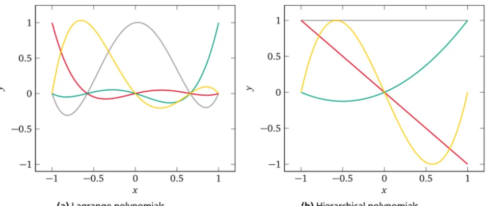
In this chapter we present a dimension-adaptive stochastic collocation algorithm based on nested collocation points. We first recall the basic concepts of the stochas-tic collocation method, both in the univariate and multivariate case. Next we show how hierarchical collocation schemes can be constructed when nested grids of col-location points are used. We then present the general form of an algorithm for the adaptive construction of hierarchical approximations. The nested collocation points of choice, i.e. Leja and Clenshaw-Curtis (CC), as well as their weighted versions, are discussed next. We proceed with the computation of statistical mo-ments, simply by post-processing the collocation-based approximation. Finally, we compare weighted and unweighted Leja and Clenshaw-Curtis (CC)-based stochas-tic collocation schemes using the stochasstochas-tic parametric waveguide model presented in Section 2.1.1.
3.1 Stochastic Collocation
In the context of the stochastic collocation method, the spectral approximation (2.24) is constructed by means of interpolation. We denote the interpolation-based approximation of the input-to-output map gwithI[g], such thatg(y)≈eg(y) = I[g] (y). The multivariate approximation I[g] is formed by combinations of univariate interpolation rules. For a sufficiently smooth mapg, the interpolation is typically based on Lagrange polynomials3.
The method employs a set of collocation pointsyj M
j=1which belong to the im-age space Ξ. We denote the set of collocation points with Z = yj Mj
=1 and its cardinality with#Z=M. There is an1−1relation between the number of collo-cation points and the number of polynomials employed in the approximation, i.e. each collocation point defines a corresponding Lagrange polynomial. The model is evaluated on all collocation points and the valuesg yj
are interpolated, resulting in the approximation I[g]. It holds that g yj
= I[g] yj
, ∀yj ∈Z, i.e. the
approximation is exact on the collocation points. Assuming that computing the model evaluationsg yj
outweighs any other op-erations in the construction of the approximation, the computational cost of the stochastic collocation method depends predominantly on#Z. The accuracy of the approximation in between the collocation points depends on the choice of interpo-lation nodes. The stochastic collocation problem based on Lagrange interpointerpo-lation can be formally defined as follows [162, Chapter 7].
3 According to L. Trefethen [154], E. Waring was the first to present Lagrange interpolation in
Definition 3.1(Stochastic collocation based on Lagrange interpolation). Let Z= {yj}Mj=1 ⊂ Ξ be a set of nodes with cardinality #Z = M and
g yj M
j=1 the set
of the corresponding model evaluations. LetP :=spanLj,j=1, 2, . . . ,M be the polynomial space of Lagrange polynomials defined byZ, where Li yj=δi j,i,j= 1, 2, . . . ,M. Then, find a polynomial approximationeg∈Psuch that
1. eg yj=g yj,∀yj∈Z, and
2. keg−gk →0asM→ ∞, in a proper norm defined onΞ.
3.1.1 Univariate Stochastic Collocation
Univariate interpolation rules are used as building blocks for the stochastic col-location method in multiple dimensions. Therefore, let us first consider the case of a single RVY. In the stochastic collocation context, any given univariate interpola-tion rule is typically defined by:
• a non-negative integeri∈N0called the interpolation level,
• a monotonically increasing “level-to-nodes” function m:N0→N which de-fines the relation between the interpolation level and the number of interpo-lation nodesmi:=m(i), wherem0=m(0) =1, and
• a grid ofmiinterpolation nodes, denoted byZi=
yi,j mi
j=1.
Denoting the univariate interpolation operator withIi, a univariate mapg(y)can
be approximated as g(y)≈eg(y) =Ii[g] (y) = mi X j=1 g yi,j li,j(y), (3.1)
whereli,jare univariate nodal Lagrange polynomials of degreepi=mi−1, defined on the gridZias li,j(y):= mi Y k=1,k6=j y−yi,k yi,j−yi,k, i6=0, 1, i=0. (3.2) We denote the corresponding univariate polynomial space withPi, such that
Pi=span
li,j,j=1, 2, . . . ,mi . (3.3)
As already mentioned, the quality of the approximation depends crucially on the interpolation nodes, which are chosen according to the univariate PDF. For exam-ple, Gauss-Legendre and Gauss-Hermite quadrature nodes are common choices for uniform and normal distributions, respectively.
3.1.2 Tensor-Product Stochastic Collocation
Moving to multiple parameters/dimensions, the simplest form of multivariate collocation consists of tensor product (TP) combinations of univariate interpolation gridsZn
inand operatorsI
n
in,n=1, 2, . . . ,N. For the ease of presentation and lighter
notation, we shall assume that all RVs are identically distributed, such thatZn in=Zin
andIn
in=Iin. The extension to the more general case is straightforward.
We introduce the multi-indexi = (i1,i2, . . . ,iN)∈NN0 which contains the inter-polation levels of all parameters. Generally, the single indicesin,n=1, 2, . . . ,N,
can have different values from one another. The special case where i1 = i2 =
· · · = iN = i is called “isotropic” TP collocation. The multivariate nodes yi,j =
yi1,j1,yi2,j2, . . . ,yiN,jN
form the tensor grid Zi:=
×
N n=1 Zin =Zi1×Zi2× · · · ×ZiN (3.4) =yi1,j1 mi1 j1=1× yi2,j2 mi2 j2=1× · · · × yiN,jN miN jN=1,with cardinality#Zi = mi1mi2· · ·miN. Denoting the corresponding multivariate Lagrange interpolation operator withIi, the TP approximation reads
g(y)≈eg(y) =Ii[g] (y) = Ii1⊗ Ii2⊗ · · · ⊗ IiN [q] (y) (3.5) = mi1 X j1=1 mi2 X j2=1 · · · miN X jN=1 g yi1,j1,yi2,j2, . . . ,yiN,jN YN n=1 lin,jn(yn) = X yi,j∈Zi g yi,j Li,j(y),
where⊗denotes a tensor product and the multivariate Lagrange polynomials are defined as Li,j(y):= N Y n=1 lin,jn(yn). (3.6)
The corresponding TP polynomial spacePiis given by
Pi=
N
O
n=1
While simple in its conception and construction, the TP stochastic collocation method has a complexity of O mN
`
, where m` = maxnmin, and therefore
be-comes intractable even for a relatively small number of parameters. The curse of dimensionality is particularly evident in the isotropic TP case, where the number of collocation points and corresponding model evaluations is exactly equal tomN
i.
3.1.3 Stochastic Collocation on Smolyak Sparse Grids Mitigating the complexity toO m`(logm`)N−1
while only mildly compromising the approximation’s accuracy is possible by employing sparse grids [27]. Sparse grids were first introduced by S. A. Smolyak in [145] for multivariate integration and interpolation purposes and have been further analyzed in the context of the stochastic collocation method in a large number of works, see e.g [6, 13, 108, 116, 163].
We introduce the non-negative integer`∈N0, called the approximation level, and the corresponding Smolyak multi-index setΛSM` , such that
ΛSM` :={i :|i|:=i1+i2+· · ·+iN≤`}. (3.8) Further introducing the difference operators
∆i:=Ii− Ii−1, (3.9)
∆i:=∆i1⊗∆i2⊗ · · · ⊗∆iN, (3.10)
whereI−1is the null operator, the Smolyak approximation formula reads g(y)≈eg(y) =ISM
` [g] (y) = X
|i|≤`
∆i[g] (y). (3.11)
The Smolyak sparse grid of multivariate interpolation nodesZSM
` is given as a
com-bination of tensor grids, such that ZSM
` = [ `−N+1≤|i|≤`
Zi. (3.12)
In its core, the Smolyak approximation formula (3.11) is nothing more than a linear combination of TP collocation formulas (3.5), where the corresponding tensor grids have a relatively small cardinality.
The original Smolyak sparse grids are of isotropic nature due to (3.8). It is easy to observe that this constraint includes equal contributions from all parameters, that is, equal maximum interpolation levels and number of univariate nodes. As illus-trated in Figure 3.1, the complexity reduction fromO mN
`
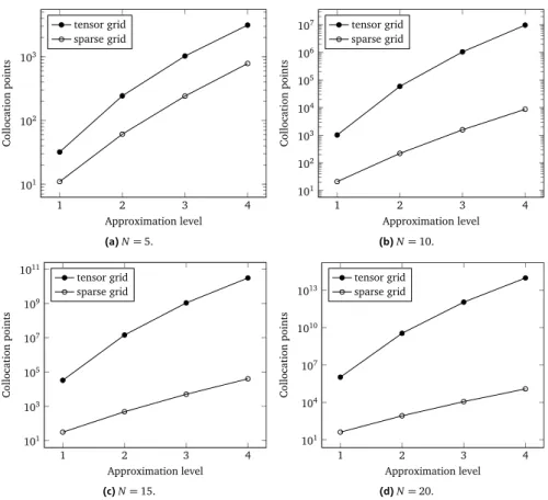
1 2 3 4 101 102 103 Approximation level Collocation points tensor grid sparse grid (a)N=5. 1 2 3 4 101 102 103 104 105 106 107 Approximation level Collocation points tensor grid sparse grid (b)N=10. 1 2 3 4 101 103 105 107 109 1011 Approximation level Collocation points tensor grid sparse grid (c)N=15. 1 2 3 4 101 104 107 1010 1013 Approximation level Collocation points tensor grid sparse grid (d)N=20.
Figure 3.1:Comparison of the complexity growth between tensor grids and sparse grids. In all 4 cases, both grids are isotropic and based on Gauss-Legendre nodes.
due to isotropic sparse grids is tremendous, however, the method is not free of the curse of dimensionality.
In practice, a QoI is rarely equally sensitive to variations from all considered parameters. This anisotropy can be exploited to construct anisotropic sparse grids [117] of reduced sizes, also referred to as “generalized Smolyak” sparse grids [6, 117, 139], as will be shown in Section 3.3.
![Figure 3.2: Nested and non-nested univariare interpolation nodes for a uniformly distributed parameter in the range [−1, 1] and interpolation levels i = 1,](https://thumb-us.123doks.com/thumbv2/123dok_us/10053296.2905024/36.629.81.576.98.324/figure-nested-univariare-interpolation-uniformly-distributed-parameter-interpolation.webp)