An Application of Master Schedule Smoothing and
Planned Lead Time Control
Chee-Chong Teo
School of Civil & Environmental Engineering, Nanyang Technological University, Nanyang Avenue, Singapore 639798, [email protected]
Rohit Bhatnagar
Nanyang Business School, Nanyang Technological University, Nanyang Avenue, Singapore 639798, [email protected]
Stephen C. Graves
Sloan School of Management, Massachusetts Institute of Technology, Cambridge, Massachusetts 02139-4307, USA, [email protected]
M
ake-to-order (MTO) manufacturers must ensure concurrent availability of all parts required for production, as anyunavailability may cause a delay in completion time. A major challenge for MTO manufacturers operating under high demand variability is to produce customized parts in time to meet internal production schedules. We present a case study of a producer of MTO offshore oil rigs that highlights the key aspects of the problem. The producer was faced with an increase in both demand and demand variability. Consequently, it had to rely heavily on subcontracting to handle pro-duction requirements that were in excess of its capacity. We focused on the manufacture of customized steel panels, which represent the main sub-assemblies for building an oil rig. We considered two key tactical parameters: the planning window of the master production schedule and the planned lead time of each workstation. Under the constraint of a fixed internal delivery lead time, we determined the optimal planning parameters. This improvement effort reduced the sub-contracting cost by implementing several actions: the creation of a master schedule for each sub-assembly family of the steel panels, the smoothing of the master schedule over its planning window, and the controlling of production at each workstation by its planned lead time. We report our experience in applying the analytical model, the managerial insights gained, and how the application benefits the oil-rig producer.
Key words: make-to-order; production smoothing; master production schedule; planned lead times; oil-rig building History: Received: April 2009; Accepted: February 2011, after 2 revisions
1. Introduction
An important competitive factor for a make-to-order (MTO) manufacturer is its ability to meet its promised delivery lead time. To achieve lead time reliability, a MTO manufacturer must have a reliable production plan for determining the procurement of raw materi-als, the production of parts, and the final assembly and testing of the end item. Typically, this production planning is based on material requirements planning (MRP) logic to coordinate the various decisions. For instance, the requirements schedule for the parts in the first tier of the bill of material is determined by offsetting the end-item assembly schedule by the planned lead time for assembly. The generation of part requirements continues for all subsequent levels of the bill of material in a similar fashion, including the procurement of raw materials.
Thus, for manufactured parts, we can view their planned lead times as an internal delivery lead time1
(IDLT) to downstream internal customers. Violations of the IDLT for any part would result in a delay in the completion time of the end item. Increasing the IDLT can buffer against uncertainties in the parts’s deliver-ies, but will result in a longer delivery lead time of the end item, which is detrimental to customer service. Ensuring availability of customized parts (for which the manufacturer cannot keep inventories) is a major challenge to most MTO manufacturers. The manufac-turer must produce these customized parts within the IDLT to meet the production schedule. In the pres-ence of a highly fluctuating demand, the MTO manu-facturer must be able to flex its production capability in periods of high demand, e.g., by overtime or sub-contracting, to meet the IDLT.
This article reports an application that addresses the aforementioned problem, wherein we propose an improved production planning framework for a pro-ducer of MTO offshore oil rigs. At the time of the application, the company had experienced a sudden 211
surge in demand due to the global increase in demand for energy. However, given the cyclical nat-ure of the industry, the firm was hesitant to invest heavily in expanding its capacity because this could result in over-capacity during the trough of the cycle. Historically, the firm’s strategy had been to use sub-contracting to handle upswings in its production requirements. This project was part of an initiative to improve the company’s production planning to reduce its subcontracting cost. We focus herein on the production planning of customized steel panels, as these represent the key sub-assemblies of an oil rig and their production is on the critical path of oil-rig building. The panel production had experienced a highly variable loading on its capacity, resulting in high subcontracting costs that were incurred to expe-dite production to meet the IDLT for the steel panels. In this article, we report our effort to improve the pro-duction planning of panel propro-duction with the objec-tive of minimizing subcontracting costs. We apply the model in Teo et al. (2011) in this case study.
We focus on how best to smooth production in the multi-station steel panel production. We consider two key planning parameters, namely the planned lead time at each workstation and the planning window. The planned lead time at a workstation projects the planned amount of time each job spends at the sta-tion. A longer planned lead time implies more time at a station, resulting in more work-in-process (WIP) at the station, but allowing for smoothing of the work-load. The planning window is the slack that reflects how much longer the IDLT is than the total planned lead time for a job. A longer planning window allows more smoothing of the master production schedule (MPS), which results in a less variable work release. In this project, we first recommended the tactics of MPS smoothing and the use of planned lead time con-trol for the individual workstations. Subsequently, we determined the optimal planning windows and planned lead times that minimize the subcontracting cost.
There is substantial literature on production smoothing in make-to-stock production, most of which focuses on the benefits of a stable capacity loading. However, there is not much work on produc-tion smoothing in the MTO context. Cruickshanks et al. (1984) consider production smoothing in a sin-gle-stage, MTO facility and introduce the concept of the planning window. Teo et al. (2011) also consider the planning window in smoothing the MPS, as well as planned lead time control in a multi-product, multi-station system. Furthermore, the article consid-ers a production system that quotes a fixed delivery lead time, which is analogous to the fixed IDLT of the customized steel panels in this case study. Indeed, the model employed in this application comes from our
work in Teo et al. The current article complements Teo et al. in that we show here with a real-life exam-ple that MPS smoothing and planned lead time control are effective tactics to improve production planning. Furthermore, we discuss the issues of implementing such tactics and develop managerial insights on the relationship between the key planning parameters. We believe this case study is representa-tive of many MTO manufacturers and thus, we expect the insights derived to be useful for practitioners. This is especially true in the light of the current trend toward mass customization, as firms increasingly need to respond to customer pressure for greater product variety. This case study is also related to work on MTO production that quotes a fixed delivery lead time. So and Song (1998) and Rao et al. (2005) determine the fixed quoted delivery lead time to max-imize profits for a single-stage system that produces an aggregate product. This article differs from both these works in that our paper is practice-based and our analysis encompasses decisions associated with the MPS and internal lead times in a multi-station, multi-product environment.
This article is organized as follows. In the next sec-tion, we review the model in Teo et al. (2011) that was applied in this case study. In section 3, we describe the process flow and the problems of planning in the panel production. We then describe in section 4 the initial study and the plans for improvement. In section 5, we present the optimization model from Teo et al. and describe how we validate the under-lying model assumptions and parameterize the model inputs. In section 6, we explain the recommendations and managerial insights based on the optimization solution. Subsequently, we validate the model output in section 7. We conclude in section 8 with a dis-cussion on how the application had influenced the company.
2. Review of Model
For completeness, we provide a high-level review of the model in Teo et al. (2011). Teo et al. consider a MTO, multi-station production system. The system produces multiple product families, each with a stochastic demand process and a fixed, guaranteed delivery lead time. The production schedule is con-trolled by the MRP-based logic, where the planned lead time at each workstation controls the production quantities. We will present the review in the context of this article, i.e., production planning to meet inter-nal orders. The “fixed guaranteed delivery lead times” and “product families” in Teo et al. corre-spond to the IDLT and sub-assembly families, respec-tively. Note that we will present only the aspects of the model that are useful to the case discussion.
2.1. Product Planned Lead Time
We begin by defining the product planned lead time PPLTk as the total planned duration that a job from sub-assembly family k takes to be completed by the
shopafter it is released into the shop. In addition, for
each workstation, we define the station planned lead
time SPLTias the planned lead time at workstationi; it
is theintendedamount of time to complete processing of each job at the workstation, including both process-ing and waitprocess-ing time. We assume each workstation has the same planned lead time for all sub-assembly families. We can expressPPLTkby:
PPLTk¼
X
i
x
ikSPLTi; ð1Þwhere xik is the number of times that each job from sub-assembly family kvisits workstation i, assuming that each sub-assembly family has a pre-determined job routing.
2.2. MPS Smoothing
The model assumes that orders arrive in each period according to a random process, with delivery dates specified by the IDLT. In addition, the MPS dictates how these orders are met. More specifically, we equate theMPSwith the release schedule to meet the orders.
Nominally, MRP logic would dictate that an order with due date t + IDLTk is released at time t +
IDLTkPPLTk. We deviate from this logic to allow the smoothing of the MPS, and hence, less variable job releases into the shop. Smoothing of the MPS for each sub-assembly familykis possible only if its inter-nal delivery lead timeIDLTkis longer than itsPPLTk. We define the resulting slack as the planning window
Wk:
Wk¼IDLTkPPLTkþ1: ð2Þ
For orders received at timet, the planning window spans fromt + PPLTktot + IDLTk. The MPS over the planning window (i.e., the production quantities to be completed over t + PPLTk to t + IDLTk) can be lev-eled, where the extent of leveling depends on Wk; a larger planning window allows for a more even spread of the MPS. We note that if IDLTk= PPLTk, then Wk= 1; this corresponds to no smoothing of the MPS since the releases in each period t must corre-spond exactly to the quantities to be completed in
t + PPLTk.
2.3. Workstation Control
Besides the variable MPS, the effective workload at the workstations fluctuates over time due to varying job arrivals and production noise, e.g., setups, yields,
and variable processing times. A longerSPLTipermits a smoother production at the workstation as it has greater flexibility to level out the variation in work-load arrivals over theSPLTi. However, with a longer
SPLTi, jobs stay longer at the workstation, which leads to a higher WIP inventory.
2.4. Optimization Model
Given that theIDLTk is fixed, the decision variables are the SPLTi, which would determine the PPLTk and Wk according to (1) and (2). Increasing the
PPLTk, i.e., allowing for longerSPLTi at the worksta-tions, leads to more smoothing for both job arrivals and production noise at the stations, but it would lead to a higher WIP inventory level. A longer
PPLTkalso implies a smallerWk, which causes a less stable job release and consequently more variable job arrival at the workstations. In addition, a longer
SPLTi not only smoothes the workload at the work-station, but also smoothes the arrivals to down-stream stations.
We now consider how the aforementioned deci-sion variables can affect the relevant production costs. We letPitbe the random variable denoting the production requirements in workhours at worksta-tion i in time period t. We interpret Pit as the pro-duction quantities required at station i in period
t that assure the work-in-queue meets the SPLTi. Furthermore, we definePitas theeffectiveproduction output as we assume it includes both scheduled workload and (unscheduled) production noise. We let ci be the penalty cost per workhour of capacity shortfall, which may represent, e.g., subcontracting cost and overtime cost; mi denotes the nominal capacity for workstation i in workhours per period;
hik represents the unit WIP inventory holding cost (per workhour per period) at workstationifor prod-uct family k; Qikt denotes the queue length in work-hours at start of t for product family k at station i. We express the expected total cost across all work-stations as: X i ciE P½ itmiþþ X k hikE Q½ ikt " # ð3Þ where x+ =max (x, 0). The term c
iE[Pit mi]+is the expected penalty cost at workstationiresulting from capacity shortfall, i.e., if Pit> mi. We assume that wheneverPit> mi, the station is always able to com-plete Pit but it incurs ci per hour for all production in excess ofmi. A more variablePitleads to a higher expected penalty cost with its variability controlled by Wk, PPLTk, and SPLTi. The termhiE[Qit] signifies the expected WIP inventory holding cost at work-station i, where a larger SPLTi yields a higher WIP inventory level.
Equation (3) forms the objective function of the optimization program that determines the optimal
SPLTiandWk. (To achieve a better flow of this article, we will defer the presentation of the optimization model to Section 5.) We compute
R
iciE P½ itmiþ bythe linear loss integral, assuming thatPitis normally distributed. In the rest of this section, we present the characterization of the first two moments of Pit required for the computation.
2.5. CharacterizingPitfor a Single Sub-Assembly Family
We first consider a single sub-assembly family and we drop the subscript k for notational convenience. We assume that the demand for each sub-assembly family is independent and identically distributed over time. For tractability, we introduce a dummy work-station to model the MPS smoothing and work release. We regard the unreleased orders as a demand queue at this dummy station, waiting to be released into the shop. The job arrival to the dummy station (station 0) in period t is the demand in t and the production output corresponds to the job release. We model the MPS smoothing by:
P0t ¼
Q0t
W ; ð4Þ
where P0t is the production output (job release) in periodt,Q0tis the queue of work at the start of per-iodtand Wis the planning window (W1). In (4), the shop releases 1/W of the on-hand orders in each period to approximate the requirement that every order does not wait more than W periods. Equation (4) models the smoothing of the release by spread-ing the on-hand orders evenly over the plannspread-ing window.
The model permits the linkage between discrete time planning and intra-period workflow. In particu-lar, it models the MPS in discrete time buckets and the arrivals and production at the station are assumed to occur over smaller time grids to permit multiple arrivals and production within each time bucket. Spe-cifically, each time periodtat stationiis sub-divided into pi equal sub-intervals, each with size Di = 1/pi. The main assumption here is that the workstation produces a fixed fraction Di/SPLTi of the work-in-queue at the start of each sub-period. The resulting production rule is similar to (4) albeit it is a function of the time grid. Effectively, the workstation i must not allow work to wait for more than SPLTi periods and thus it must process close to Di/SPLTi of the work-in-queue in each sub-period. In addition, to achieve tractability, the work arrival at the worksta-tion in periodt, which we denote asAit, is assumed to be uniform within each period t; that is, the arrival
amount at the start of each sub-period is equal to
Ait/p.
Teo et al. derive an expression for Pit, which is given by:
Pit¼biðiÞQitþ
c
iðiÞAit; ð5Þwhere the coefficients b(Di) and c(Di) are expressed as: biðiÞ ¼1½1ði=SPLTiÞpi and
c
ið Þ ¼i 1biðiÞ 1ði=SPLTiÞ 1=SPLTi ð Þ : ð6ÞEquation (5) expresses the production in each time period as a linear function of both the work queue at the start of the period and the arrivals during the per-iod. The sub-intervalDireflects the size of underlying time interval for job movements at workstation i, where Di is set on the order of the average inter-arrival time. If the workflow is of a high enough frequency, the workflow can be approximated as a fluid-like workflow by considering the continuous time limits for bi(Di) and ci(Di) as Di goes to zero. The continuous time limits of bi(Di) and ci(Di) are given by:
bið!0Þ ¼1e1=SPLTi and
c
ið!0Þ ¼1SPLTibi:ð7Þ Teo et al. show by a simulation study that accurate model output can be achieved if the appropriate co-efficients are employed.
2.6. Workflow Model
The workflow model links the MPS smoothing and the network of workstations so as to capture their in-terdependencies. We assume that each workhour of production at station j generates uij workhours of input to station i on average. We model the work arrivals to stationiby
Ait¼
X
j
u
ijPjt: ð8ÞFor the dummy station (station 0), we note thatui0
is the average amount of work that starts at worksta-tioni for each new job. Furthermore, we express the balance equation at workstationias:
Qit¼Qi;t1Pi;t1þAi;t1þfit; ð9Þ
where fit denotes the random production noise at
workstationi. By expressing (5), (8), and (9) in matrix-vector form, Teo et al. then obtain the matrix-vector of expec-tation ofPitandQit, and covariance matrix ofPitfor all stations, namelyE[P],E[Q],andVar(P),respectively.
To extend the single-family model to accommodate multiple assembly families, we model each sub-assembly family the same way as in the single-family model, i.e., each product family k has an MPS and each family has its own demand process, routings, and production noise. The single-family model char-acterizes the production requirements and WIP inventory for sub-assembly family k, i.e., E[Pk], Var (Pk), and E[Qk]. We can obtain the expectation of the total production requirements and WIP inven-tory by aggregating across all sub-assembly families: E½Ptotal ¼
P
kE½ Pk and E½Qtotal ¼
P
kE½ Qk. If
demand is independent between the sub-assembly families, we can obtain the variance of the total pro-duction requirements:
VarðPtotalÞ ¼ X
k
VarðPkÞ: ð10Þ
We can relax the assumption of independent demand by incorporating demand correlations between the sub-assemblies into (10) (refer to Teo [2006] for details).
3. Panel Production: Process Flow and
Challenges
The company is a producer of customized jack-up oil rigs. Jack-up oil rigs are offshore rigs that are mobile in water, and can anchor themselves by deploying jack-like legs. The fundamental structure of the oil rig is the hull, which is the platform on which most facili-ties of the rig are built. A typical hull consists of steel blocks; each steel block is constructed by joining steel structures called panels. A block commonly consists of 10 to more than 60 panels. The steel panel repre-sents the most elementary sub-assembly in the hull construction. A panel is built using one or more steel
plates, with outfitting components welded onto it to strengthen the structure.
There are three sub-assembly families in the panel production: Big Panels,Small Panels, and Outfits. Big
Panels are panels built by joining two or more steel
plates, while theSmall Panelsare built using a single steel plate. The size of the panels varies widely with the weight of a panel ranging from 0.5 to 10 tons. The
Outfits are the outfitting components welded onto
the panels. Figure 1 shows the process flow map for the panel production.
At theBlaststation, raw plates are “blasted” by ball grids to remove surface impurities, followed by the application of a corrosion preventive coating. The typ-ical raw steel plate is 1.5 m wide, 8 m long, and has a thickness of¼–¾inch. The blasted plates are sent to
theNC Gas CutorNC Plasma Cutstations to be cut to
the required dimensions. The NC Gas Cut station is capable of cutting both thin and thick plates, while
the NC Plasma Cut station can only cut thin plates.
TheBig Panels require thick plates and are therefore
sent to the NC Gas Cut station. The Small Panels
require thin steel plates but are processed at the NC
Gas Cutstation to balance the workload between the
two stations. For the same reason, although theOutfits
also require thin plates, a fraction of theOutfitsare cut in theNC Gas Cutstation while the rest are processed at theNC Plasma Cutstation. After cutting, the parts remain joined to the steel plate by connectors called “bridges,” and these are manually cut at the Bridge Cutstation.
Subsequently, the plates for each sub-assembly family follow different process routes. The thick plates for the Big Panels are beveled at the Bevel
station, and then go through a series of welding processes at the Tack and Join stations to join the plates to form the basic panel structure. The panels are then paint-marked at theMark station to indicate
Big Panels: Blast NC Gas Bridge Cut Bevel Tack Join Mark Outfitting (Big Panels)
Small Panels: Blast NC Gas Bridge Cut Mark Outfitting (Small Panels)
Outfits: Blast NC Plasma or NC Gas Bridge Cut Profile Shop Outfits (both Big and Small Panels)
Blast
NC Gas Cut
Bevel Tack Mark
Outfitting (Small Panels) Outfitting (Big Panels) Bridge Cut NC Plasma Cut Outfits SmallPanels Join Raw steel plates Profile Blasting Shop Shop NC Panel Shop
the positions of theOutfitsto be fitted. Eventually, the
Big Panelsare moved to theOutfitting(Big Panels)
sta-tion to weld theOutfits. Since theSmall Panelsare built using a single plate, no welding is needed and they are moved directly to the Mark station and sub-sequently to the Outfitting(Small Panels) station. The
Outfitsare sent to theProfile Shopfrom theBridge Cut,
where the cut steel parts undergo some simple metal forming operations to produce the outfitting compo-nents. Finally, theOutfitsare transferred to either the
Outfitting (Big Panels) or the Outfitting (Small Panels)
to be fitted onto their corresponding panels. The com-pleted panels are then ready for quality checks before moving downstream to construct the steel blocks.
The panel production shown in Figure 1 occurs in three separate shops, namely the Blasting Shop, NC
Shop, and Panel Shop, which are physically located
next to each other. The Blasting Shop consists of the
Blast station, the NC Shop has the two NC cutting
stations, and the Panel Shop includes the rest of the processing stations. Production control for the panel production had been based on the planned lead times at the shop level. The planned lead times for the
Blast-ing Shop, NC Shop, and Panel Shop were 5, 8, and
13 days, respectively, resulting in an IDLT of 26 days for the panel production; that is, the panel production facilities need to deliver each internal order of panels exactly 26 days after receipt of the order.
Any delay in delivering the panels hinders the downstream assembly for the steel blocks, which might in turn affect the meeting of the promised oil rig delivery dates. The progress of jobs is monitored against the shops’ planned lead times to approximate whether or not jobs are able to meet the delivery sche-dule. In times of high capacity loading, jobs are sub-contracted to vendors to keep them from falling behind their planned lead times. Most of these ven-dors are located close by or within the panel produc-tion facility itself. While the producproduc-tion schedule of
the Panel Shop is monitored based on the shop’s
planned lead time, work can be outsourced at each of its individual workstations. Production planning relies on a single MPS for all sub-assembly families. In addition, there is no regulation of the MPS and the job release, whereby jobs are released once the orders are received from the downstream internal customers. With the surge in demand, most workstations in the production shop experience a heavier and more vari-able workload, which results in rising subcontracting costs. The company sought to increase its utilization of in-house capacity and to reduce subcontracting costs.
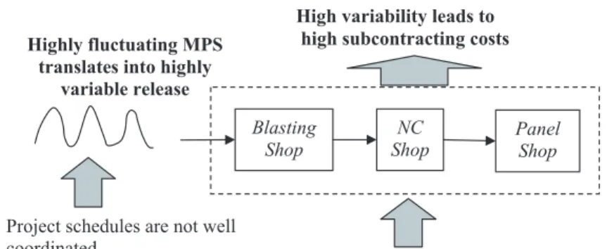
The management identified that one cause of the variable workload was the highly fluctuating MPS. The MPS was highly variable for three reasons. First, the production schedules of panels for the different oil-rig projects were not well coordinated. As a result, the total internal demand for panels was quite vari-able and resulted in varivari-able work release. Second, raw steel plates of required thickness and grades were frequently unavailable, and this delayed the release of some panels. Third, the raw steel plates were stacked to conserve space and therefore, finding the required plate often took substantial time; this added consider-able variability to the picking time of the raw plates. In addition to the varying MPS, another cause for the large workload variability was the diverse processing requirements at the workstations, due to the different sizes of plates as well as the different number of plates and outfitting components required for each panel. The challenges in the panel production are illustrated in Figure 2.
The management recognized that addressing these causes could lead to a reduction in production vari-ability. However, they believed that this would require a long-term effort and would depend on fac-tors external to the company. Coordination of the project schedules would involve coordination
Blasting Shop
NC
Shop Panel Shop
• Project schedules are not well
coordinated
• Raw steel plates are often unavailable
• Much time needed in locating plates
Diverse processing requirements
Many different cut dimensions of plates, as well as variable number of plates and outfitting components for each panel
High variability leads to high subcontracting costs Highly fluctuating MPS
translates into highly variable release
between the company’s various departments as well as with its customers on delivery schedules. Improv-ing availability of raw steel plates would need better coordination with suppliers and more accurate fore-cast of global steel supply. Shorter picking times for steel plates would require considerable capital investment and time to devise new ways or equip-ment for material handling. Reducing the diverse processing requirements would need standardization of panel types, which would involve setting restric-tions on oil-rig customization that might be detri-mental to customer satisfaction. The management decided that to reduce subcontracting cost within the short term, they should focus on tactical improve-ments.
The panel production highlights the problems faced by many MTO manufacturers in producing custom-ized parts to meet a production schedule. The charac-teristics of the panel production encompass various operational aspects that can be found in many pro-duction systems: a highly variable MPS, multiple product families and process routes, dissimilar pro-cessing requirements, and expediting actions taken to meet delivery schedules.
4. Initial Study and Recommendations
The company learned about the concepts of MPS smoothing and lead time control from our work in Teo et al. (2011) and wished to explore if the tactics would be of help to improve the company’s perfor-mance. A team was formed, consisting of the authors and personnel from the production department. After a careful study of the model, the production person-nel were particularly interested in two potential improvement areas as follows.
4.1. Smoothing of MPS
The production personnel recognized that a smoother MPS results in a less variable release and conse-quently fewer occurrences of “spikes” in capacity loading. The company became interested in finding out how the MPS can be smoothed in the panel pro-duction. The team recognized that the MPS can be smoothed over the planning window for each sub-assembly family if itsIDLTkto its internal customer is longer than itsPPLTk.
One seemingly obvious solution was to increase the
IDLTkto allow a longer planning window andPPLTk. However, the management did not wish to change the current internal lead time for panel production of 26 days, as the panel production is on the critical path of oil-rig building and they did not want to affect the delivery schedule of the oil rigs. Therefore, the team had to find other ways to smooth production given the fixedIDLTk.
Initial recommendation 1. Upon studying the process flow, the team identified that the Small Panels and Outfits require fewer processing steps than the Big Panels. Thus, if each sub-assembly family has its own MPS and is planned separately, each of the Small Panels and Outfits would have
a much shorter PPLTk. Hence, given that the IDLTkis the
same for each family, the planning window Wkwould be
considerably large for both sub-assembly families to perform substantial MPS smoothing. Thus, it was recommended that an MPS is created for each sub-assembly family.
4.2. Smoothing at Stations
The team recognized that the production control in
thePanel Shophad been based on the shop’s planned
lead time, rather than for its individual workstations. As a result, subcontracting decisions were often “guesswork” of predicting if a job could be completed in time to meet its due date. Furthermore, the planned lead times for the three shops were set based upon the experience of the production planners without any analytical basis.
Initial recommendation 2. The team recommended a
station planned lead time SPLTifor each workstation in the
Panel Shop, whereby the progress of jobs could be tracked more precisely. The team also identified an opportunity to achieve a smoother workflow by determining the optimal values of SPLTi.
4.3. Planning Decisions
The team then looked into the planning parameters and trade-offs in the panel production. We found that we could omit the holding cost of the WIP inventories from our analysis. We note that the exclusion of WIP inventory holding cost differs from Teo et al. and other earlier work on setting planning lead times, which consider the trade-off between capacity requirements and WIP inventory. The pri-mary reason for excluding the WIP inventory is that the total inventory held by the firm is insensitive to the planning decisions under consideration. The majority of raw steel plates required for the entire oil rig are purchased before the start of each project, so the material cost of the steel plates represents a sunk cost, i.e., it is incurred regardless of how we release work into the production shop. Furthermore, since the IDLT is fixed, the raw plates stay in the production system for approximately the same dura-tion no matter how the plates are scheduled. In addi-tion, the team found that the value added to the jobs through processing (and hence the incremental hold-ing cost) is significantly less than the subcontracthold-ing cost.
The team re-evaluated the key trade-offs and iden-tified the following planning considerations for the panel production:
•
The team needed to set the planning windowWk and the SPLTi of each workstation (which determines PPLTk). The planning window smoothes the MPS (and release) and the PPLTk (i.e., the sum ofSPLTi) smoothes both the arriv-als and the noise due to the variable processing times at the workstations.
•
Without considering the WIP inventory, the decision is to allocateSPLTi among the worksta-tions solely to minimize the total subcontracting cost. The subcontracting cost incurred at each workstation depends on its unit subcontracting cost, nominal capacity level, and variability in job arrival, and processing times.•
In this multi-station, multiple-family setting, the team needed to take into account the interde-pendence of workflow among the stations as well as among the sub-assembly families.The team recognized that the main features of the panel production could be modeled by Teo et al.: production control using planned lead times, influence of MPS smoothing on production work-flow, variability at the workstations as well as subcontracting production to meet the capacity shortfall. However, before applying the analytical model, we also considered other simpler alter-natives. For example, the team considered setting
the SPLTi of all stations to be proportional to each
station’s utilization rate while satisfying the IDLT constraints. The rationale behind this method was that the more heavily utilized stations would need longer station planned lead times. However, this method would not be able to account for many important aspects of the scenario, e.g., the variabil-ity of demand and processing requirements, the dif-ference in subcontracting cost between stations and the interdependencies of workflow between sta-tions. The team also considered the alternative of using a discrete-event simulation. However, they found that simulation was not suitable for the extensive “what-if” analysis they would like to per-form, as it would be slow to make the numerous simulation runs, especially the runs requiring opti-mization. Furthermore, the management preferred a method that did not require an extensive learning process for its personnel. As our model was formu-lated and solved in MATLAB, the management thought that the planners and engineers could read-ily learn how to use it. In addition, the model parameters, e.g., unit subcontracting cost, workflow, and capacity levels, could be easily altered accord-ing to actual changes. Moreover, MATLAB pro-vided an optimization toolbox that could be used to find the optimal planning windows and station planned lead times.
5. Model Application
5.1. Optimization ModelWe present the optimization model from Teo et al. (2011) but our objective in this application differs in that we minimize just the expected total penalty cost in (3) (i.e., we exclude the WIP inventory holding cost). The decision variables are the SPLTi of each workstation and planning windowsWk of each sub-assembly family k. The discrete time period tof the model is one day, which is the time bucket used in the existing planning system.
MinX i ciE½Pitmiþ s:t:X i SPLTiþWk1¼IDLTk;8k ð11Þ Wkak;8k ð12Þ SPLTibi;8i ð13Þ
To evaluate the objective function, we need to determine the variances of the random variablesPit; these depend on the workstation’s SPLTi (5 and 6), theSPLTi of its upstream workstations and the plan-ning windows Wk. Constraint (11) combines (1) and (2), which defines the relationship betweenWk,SPLTi, and IDLTk, where IDLTk are fixed at 26 days for all sub-assembly families. We note that in (11), xik = 1 for alli andksince every job visits each workstation once. Constraints (12) and (13) assure a lower bound of at leastakand bi on theWkand the SPLTi, respec-tively. Lower bounds ofSPLTiand planning windows are needed to avoid excessively frequent monitoring to track the job progress and the MPS. We set bothak and bi to be 1 day, as the planning time bucket of 1 day was the minimum duration that the manage-ment perceived to be suitable for planning within this highly dynamic system. The decision variables were not restricted to be integers, as non-integer values were acceptable for production control. The team set theSPLTis of theProfile Shopwhich produces the
Out-fits, to be fixed at 2 days, as the station’s processing time is relatively stable and reasonably independent of the workload.
As reported in Teo et al., we have not been able to determine whether or not the objective function is convex. Therefore, we cannot assert that the solutions are global optimal. In this exercise, we solved each test problem using many different starting points. We attained the same solution for each test problem, which increased our confidence that we had obtained a global optimum.
5.2. Validation of Model Assumptions
The team validated the following assumptions in Teo et al. for the current study.
5.2.1. Capacity Assumptions. Equation (3) assumes that every workstation is always able to meet the production requirements, although it incurs addi-tional cost per workhour of capacity shortfall. In the panel production, subcontracting is routinely used to expedite work to meet the production require-ments. Since the subcontracting is performed in nearby shops and by on-site contract workers, rela-tively little time is wasted in transporting the jobs. Furthermore, from the management’s experience, there are very few occurrences where the subcon-tractors failed to produce the outsourced demand within the SPLTi. The team also examined the assumptions for the nominal capacity mi. To apply (3), mi must be measurable and its value assumed to be constant. It is straightforward to measure mi for
NC Gas Cut and NC Plasma Cut stations as both are
machine constrained. We observed that the other stations operate with skilled workers, some of whom are cross trained to work at more than one station. Thus, there is some flexibility in allocating workers to the heavily loaded stations, which somehow dis-agrees with the assumption of constant nominal capacity. However, the team found that such re-deployment of workers was infrequent after the company experienced the high capacity loading due to the demand increase. This is because the stations with cross-trained workers become heavily loaded at the same time, thus preventing labor re-allocation.
5.2.2. Workflow Assumption. In deriving (5), the arrival to the workstation is assumed to be uniform within each time period t. However, in the panel production, jobs start to move to the next station upon completion and therefore the arrival at the downstream station is not exactly uniform within each period. Teo et al. validate this assumption via a simulation model wherein jobs move to the next station immediately after completion. The study shows that the simulation results are close to the model output despite relaxing the uniform flow assumption; the errors are small provided that the appropriate production function (i.e., either the sub-interval function (6) or the continuous-time function (7)) is chosen at each workstation according to the average flow rate. The average percentage differ-ence between the simulation results and the model output is 2.3% for all test problems and the maxi-mum error is 6.5%. The study also establishes the range of average flow rates that (6) or (7) should be
selected. The team observed that the arrival rates are low at Join, Mark and both the Outfitting
stations, as these stations assemble or process pan-els rather than plates and Outfits. As a result, the arrival rates at these stations fall within the range of flow rates found in the simulation study that necessitates the use of the sub-interval function (6). Thus, we employed the sub-interval function for these stations. The other stations have sufficiently high flow rate to justify the continuous-time assumption and hence the continuous-time function (6) was utilized.
5.2.3. Production Assumption. The development of (5) assumes that the workstation is regulated to produce a fixed fraction of the work-in-queue to sat-isfy itsSPLTi, even if capacity is available to produce the entire work-in-queue. In the panel production, the job start times at NC Plasma, NC Gas,Tack, and Join
stations are scheduled to coordinate with the receipts of engineering drawings for cutting and welding (which is similar to the synchronization of part requirements in MRP logic). Furthermore, due to the large physical size of the jobs and the space con-straints in the facilities, the stations usually produce just to meet the SPLTi, so as to avoid taking up the downstream shop space unnecessarily. To compute the total penalty cost in (3) (that forms the objective function) using the normal linear loss integral, Pitis assumed to be normally distributed. To validate this assumption, we constructed normal probability plots for the daily production output from a 2-month data and the plots showed that this assumption is reason-able.
5.2.4. Demand Assumption. In contrast to the assumption of stationary demand, the observed demand for each sub-assembly family is generally non-stationary. However, if the time horizon is considered as successive time segments, with each segment representing a constant number of oil rigs in production in their respective stable project phase, we observed that the demand is stationary within each time segment. Each time segment typically ranges from about 15 to 45 days. In addition, the daily demand data showed a fairly constant coefficient of variation (standard deviation mean) of demand within each segment. We show the demand data for
theBig Panelsover a 3-month period in Figure 3.
To test the sensitivity of our solution to the non-stationary demand, the mean demand for each
sub-assembly family was set to be either 100% or 125% of the original mean demand while keeping the demand coefficient of variation constant. The analysis showed that for all eight test scenarios, the subcon-tracting cost resulting from the original demand’s
optimal station planned lead times is no more than 4% higher than the test scenarios’ minimum subcon-tracting cost.
5.3. Data Collection
We discuss the data required for the model inputs, and how we obtain and parameterize the relevant data.
5.3.1. Capacity. To measure the nominal capacity levelsmi, we observed the throughput rate in periods of high demand, when most stations were operating at full capacity. We approximate mi by the mean throughput (in hours) per day observed in these periods.
5.3.2. Subcontracting Cost. The vendors quote the subcontracting costs in terms of cost per metric ton. Since workload in our model is measured in hours, we had to convert the subcontracting cost at each station into average subcontracting cost per workhour ci. We approximated the average subcon-tracting cost based on the average weight of the jobs at the station (in metric tons) and the mean processing time of the jobs (in hours).
5.3.3. Demand. We obtained the mean and stan-dard deviation of the internal demand for each sub-assembly family from an 8-month demand record. We found a low correlation coefficient of 0.13 between the demands ofBig PanelsandSmall Panels. However, the correlations betweenBig PanelsandOutfitsas well as between Small Panels and Outfits, are high with
correlation coefficients at more than 0.70. We modeled correlated demands between product families for (10) by incorporating the demand correlations.
5.3.4. Effective Processing Times. We acquired the mean and variance of the effective processing times (in hours) at each station from data collected in a 2-month period. We needed the mean processing times to define the workflow matrix consisting ofuij, which defines the average amount of work that each unit of production at a station generated for each downstream station. The variance of the processing time at each station is required to calculate the zero-mean noise termnitat each station. We computed the
noise due to the variability of processing time by: VarðnitÞ ¼Expected number of jobs at stationi
Variance of processing time
6. Results and Insights
We report the optimization results as well as the cor-responding expected subcontracting work and costs in Table 1. The subcontracting costs presented herein have been scaled to protect the company’s confiden-tial data, but the insights drawn are identical to the conclusions based on the actual data.
With a separate MPS for each sub-assembly fam-ily, there is a greater flexibility to adjust the planning windows of each sub-assembly family for a smoother release. The solution suggests that there should be substantial smoothing for the release of
Small Panels and Outfits, with planning windows equal to 10.8 and 9.8 days, respectively. The plan-ning window for Big Panel is 1 day, meaning no smoothing of its MPS.
The solution suggests that theSPLTiofBlastshould be reduced from 5.0 to 1.0 day, and NC Gas Cutand
NC Plasma Cut from 8.0 to 4.4 days. A proportion of
the originalSPLTiat these stations acts as safety time to buffer against the uncertainties of unavailable steel plates and the long picking times. For the Small
Pan-els and Outfits, most of the excess days from this
reduction are reallocated to their planning windows. Here, the planning windows would not just smooth the MPS but also act as the safety times for acquiring steel plates. For the Big Panels,theSPLTiof the Blast station is mainly reallocated to the other work-stations.
The optimal SPLTi at theJoinstation is the largest among the workstations at 7.8 days. We observed that the utilization rate at the Join station is more than 90%; its processing time is also highly variable, with a coefficient of variation of 0.76. The optimalSPLTis of
Outfitting (Big Panels)andOutfitting (Small Panels)are
also high at 6.6 days, but still lower thanJoin, despite both stations having higher utilization rates and co-efficient of variation for their processing time. The reason is that the larger SPLTi at the Join station would smooth the production output, which in turn would lead to smoother arrival at the downstream
Outfitting (Big Panels) and Outfitting (Small Panels).
The solution also suggests that Bevel,Tack, and Mark
stations have the shortest station planned lead times of 1.0 day due to their comparatively lower utiliza-tion. Even with a station planned lead times of 1.0 day, the expected subcontracting costs are low at these stations.
By exercising the model for different what-if sce-narios, the team developed the following insights for
setting the planning windows and station planned lead times:
•
The team gained insights on the interaction between the planning windows and the station planned lead times. A longer planning window is preferred if a sub-assembly family faces a highly variable demand and relatively lower workload variability at the stations. On the other hand, if the variability of processing time at the stations is relatively larger, longer station planned lead times are preferred to smooth pro-duction at the workstations.•
A workstation would require a longerSPLTiif it faces greater variability in processing require-ments, has higher utilization rate and/or unit subcontracting cost. The management had previ-ously thought that the SPLTi should be based only on the utilization rate.•
Smoothing at an upstream station has the added advantage of smoothing the arrivals to down-stream stations. The management learned that looking at each individual station in isolation is suboptimal.We note that in situations where the WIP holding cost is significant, one also has to consider that longer
SPLTis lead to higher WIP inventory levels. The above insights are useful for understanding the trade-offs among capacity, lead time, and production smooth-ness.
7. Validation
The team attempted to validate the predictive capa-bility of the model, i.e., the accuracy of the model in characterizing the panel production. The most useful validation would be to compare the actual amount of work subcontracted out with that predicted by the
Table 1 Optimization Results
Station Original Wkor SPLTi Optimal Wkor SPLTi
Expected subcontracting work (hours/day)
Expected subcontracting cost ($/day)
Planning window for Big Panels 1.0 1.0 – –
Planning window for Small Panels 1.0 10.8 – –
Planning window for Outfits 1.0 9.8 – –
Blast 5.0 1.0 0.13 73 NC Gas Cut 8.0 4.4 0.37 155 NC Plasma Cut 8.0 4.4 0.12 60 Bridge Panel Sho p 13 : 0 3.1 0.12 143 Bevel 1.0 <0.01 <1 Tack 1.0 <0.01 <1 Join 7.8 5.96 775 Mark 1.0 <0.01 <1
Outfitting (Big Panels) 6.6 5.83 874
Outfitting (Small Panels) 6.6 4.39 351
m
model. However, the subcontracting decisions in the
Panel Shopwere based on the aggregate planned lead
time of the shop. In our model, production control is set based on the SPLTi of individual stations. Thus, the above comparison could not be made for the
Panel Shop and unfortunately, this is where most of
the workstations are located. For the Blasting Shop
and NC Shop, we found that the amount of
subcon-tracted work predicted by the model is about 26% and 21%, respectively, lesser than the actual data for the two stations. The team viewed this as a reason-able validation given the presence of high variability in the system and the somewhat incomplete subcon-tracting data, since the company did not keep an organized record of subcontracting cost incurred at
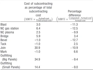
each workstation. After the recommendation to assign the SPLTi to individual stations was imple-mented, new and more comprehensive data on sub-contracting costs became available. We re-validated the predictive capability of the model and found that the model output is about 9% lower than the actual costs; this error is significantly lower than the initial limited validation using data only from the Blasting
Shop and NC Shop. The corresponding percentage
difference at each workstation is shown in Table 2. In the same table, we also present the actual cost at each workstation as a percentage of the total actual cost to show the relative significance in cost at each workstation.
Before implementing the recommendations, the management needed to gain confidence in the results. Given the incomplete subcontracting data at the time, the team first attempted to determine rough-cut potential savings that would result from these changes. The team attempted to compare the actual subcontracting cost with that computed by the model. To accommodate the model’s predictive error, we adjusted the computed subcontracting costs for the Blasting Shop and NC Shop. Specifically, we modified the computed subcontracting cost by the percentage error determined through our validation of the model’s predictive capability (i.e., the aforementioned errors of 26% and 21%, respectively) by:
As stated earlier, we could not determine the computation error at thePanel Shop. We use the per-centage errors at the Blasting Shop and NC Shopas a guide and set the Panel Shop’s percentage errors to be in the range 18–30%. Comparing the resulting adjusted optimal total subcontracting costs with the actual average historical cost, we estimated that the recommendations would result in a 20–30% cost reduction, which is acceptable to the management.
In another effort to estimate the potential cost sav-ings, the team input the currentSPLTis into the model and compared the resulting total subcontracting cost with the optimal cost. However, the individual sta-tions in thePanel Shophad not been assignedSPLTi. To overcome this, the current cost was estimated by setting theSPLTiof the stations in thePanel Shop pro-portional to the station’s utilization rate while satisfy-ing thePanel Shop’s planned lead time of 13 days. The results from this comparison showed that the optimal solution would reduce the cost by about 21.8%. We also compared the optimal cost with that of another alternative in which theSPLTis ofallstations were set proportional to each station’s utilization rate while satisfying the IDLT constraint. By inputting theSPLTi based on this alternative into the MATLAB program, we found that the total expected subcontracting cost for this alternative is 14.4% higher than that of the optimal expected cost. We regard the abovemen-tioned comparisons as conservative estimates of the true savings. This is because the actual production control of the Panel Shop was based on the shop’s planned lead time, rather than the more accurate con-trol using the SPLTis of individual stations as assumed in the comparison.
Table 2 Percentage Differences Between Actual Cost and Computed Cost Per Day (After AdoptingSPLTiat Individual Workstations)
Cost of subcontracting as percentage of total
subcontracting cost
100% Actual cost Total actual cost
Percentage difference
100%ComputedActual costActual cost
Blast 3.0 11.3 NC gas station 6.4 12.5 NC plasma 2.5 9.9 Bridge 5.9 3.4 Bevel <1.0 12.7 Tack <1.0 2.5 Join 30.9 10.9 Mark <1.0 6.6 Outfitting (Big Panels) 34.9 9.4 Outfitting (Small Panels) 14.4 9.0
Adjusted subcontracting cost¼ 100%
100%þPercentage error
The major limitation of our model is that it does not account for rush orders of urgent panels. These panels are crucial components for the downstream steel blocks and their late completion would lead to serious delays in the steel block production. These orders are processed immediately upon arrival and are fre-quently subcontracted to expedite their completion. Typically, each order is subcontracted at some selected stations depending on the order’s processing requirement; therefore the rush orders do not have distinct flow paths but have numerous processing routes. Hence, even though we had explored over-coming this limitation by defining the rush orders as separate product families, we faced difficulties in accurately capturing the rush orders with our existing shop data. Nevertheless, the management concluded that the collected data, model assumptions, and results were reasonable and that our model serves well for tactical planning since it is able to capture the core features of the problem.
8. Influences on Company
The company adopted the recommendations of creat-ing a MPS for each sub-assembly family and individ-ual planned lead times for each station. In particular, each MPS is smoothed over the planning window with the job releases leveled, and the company uses the station planned lead time to monitor the progress of jobs at each workstation to determine whether or not a job should be subcontracted. More specifically, the shop managers monitor the job progress by approximating completion time of newly arrived jobs at each workstation based on estimation of total pro-cessing times of the jobs in queue.
Before implementing the recommendations for the values of the planning windows andSPLTis, the com-pany decided to add production capacity as it observed a continuous growth in oil-rig demand and projected that the growth was sustainable. However, the company did not acquire excessive amount of capacity to buffer against demand variability but chose to maintain the strategy of subcontracting. Therefore, instead of implementing the precise recom-mendations for the values of planning windows and
SPLTis as a static solution, the company utilized the model to support the monthly updating of the values in response to the continual changes in production capacity. Furthermore, since the model requires large amounts of data as inputs, the use of the model is helped by the company’s new initiative to regularly update shop data.
The company also employs the model for what-if analysis to support planning; for instance, the model
is used by the company to determine how capacity addition affects subcontracting cost. In addition, the model is also used as a guide for focusing improve-ment efforts. The model helped to identify steel avail-ability and production scheduling as two potential areas in which subcontracting cost could be reduced; consequently, there were projects carried out to address these issues (see Huang [2006] and Tan [2006] for details of these projects). Another significant result is that the project has led to greater awareness of the importance of considering the interrelationship among lead time, capacity, and production smooth-ness. Furthermore, there is now a greater emphasis on reducing variability of production. However, we were not able to quantify the resulting savings in subcon-tracting cost because of the ongoing changes in the production shop and oil-rig demand, as well as fluc-tuations in global steel supply, and subcontracting charges.
Acknowledgments
This research has been supported by the Singapore-MIT Alliance (SMA) program. The authors thank the Depart-mental Editor, Senior Editor, and two anonymous referees for their valuable comments, which greatly improved the article.
Note 1
Note that we use the term internal delivery lead time (IDLT) to represent the total planned lead time of producing a part or sub-assembly needed for downstream processes. References
Cruickshanks, A. B., R. D. Drescher, S. C. Graves. 1984. A study of production smoothing in a job shop environment.Manage. Sci.30(3): 36–42.
Huang, F. 2006. Production Scheduling in a Make-To-Order Job Shop under Job Arrival Uncertainty. Unpublished Master’s Dissertation, Department of Mechanical Engineering, MIT, Cambridge, MA.
Rao, U. S., J. M. Swaminathan, J. Zhang. 2005. Demand and pro-duction with uniform guaranteed lead time. Prod. Oper. Manag.14(4): 400–412.
So, K. C., J.-S. Song. 1998. Price, delivery time guarantees and capacity selection.Eur. J. Oper. Res.111(1): 28–49.
Tan, C. Y. 2006. Inventory Management of Steel Plates at an Oil Rig Construction Company. Unpublished Master’s Disserta-tion, Department of Mechanical Engineering, MIT, Cam-bridge, MA.
Teo, C. C. 2006. A Tactical Planning Model for Make-To-Order Environment under Demand Uncertainty. Unpublished Doctoral Dissertation, Singapore-MIT Alliance, Nanyang Technological University, Singapore.
Teo, C. C., R. Bhatnagar, S. C. Graves. 2011. Setting planned lead times for a make-to-order production system with master schedule smoothing.IIE Trans.4(6): 399–414.