SFB
823
Power of change-point tests
for long-range dependent
data
Discussion Paper
Herold Dehling, Aeneas Rooch,
Murad S. Taqqu
POWER OF CHANGE-POINT TESTS FOR LONG-RANGE DEPENDENT DATA
HEROLD DEHLING, AENEAS ROOCH, AND MURAD S. TAQQU
Abstract. We investigate the power of the CUSUM test and the Wilcoxon change-point tests for a shift in the mean of a process with long-range dependent noise. We derive analytic formulas for the power of these tests under local alternatives. These results enable us to calculate the asymptotic relative efficiency (ARE) of the CUSUM test and the Wilcoxon change point test. We obtain the surprising result that for Gaussian data, the ARE of these two tests equals 1, in contrast to the case of i.i.d. noise when the ARE is known to be 3/π.
Contents
1. Introduction 1
2. Power of the CUSUM Test under Local Alternatives 3 3. Power of the Wilcoxon Change-Point Test under Local Alternatives 6 4. ARE of the Wilcoxon Change-Point Test and the CUSUM Test for LRD Data 12 5. ARE of the Wilcoxon Change-Point Test and the CUSUM Test for IID Data 16
6. Simulation Results 22
6.1. Gaussian data 22
6.2. Heavy tailed data 23
References 25
1. Introduction
Statistical tests for the presence of changes in the structure of time series are of great importance in a wide range of scientific discussions, e.g. regarding economic, technological and climate data. Many procedures for detecting changes and for estimating change-points have been proposed in the literature; see e.g. Cs¨org˝o and Horvath (1997) for a detailed exposition. In the case of independent data, the theory is quite satisfactory. For various types of change-point models, statistical procedures have been proposed and their properties investigated. In constrast, the situation is different for dependent data, such as encountered in time series models. For dependent data, most research has focused on linear procedures, such as cumulative sum (CUSUM) tests, and there are many open problems when it comes to other types of test procedures, e.g. those used in robust statistics.
In the present paper, we study the change-point problem for long-range dependent data. Specifically, we will test the hypothesis that the process is stationary against the alternative that there is a change in the mean. The classical test statistic for this problem is the CUSUM
Key words and phrases. Change-point problems, nonparametric change-point tests, Wilcoxon two-sample rank test, power of test, local alternatives, asymptotic relative efficiency of tests, long-range dependent data, long memory, functional limit theorem.
Herold Dehling and Aeneas Rooch were supported in part by the Collaborative Research Grant 823, Project C3 Analysis of Structural Change in Dynamic Processes, of the German Research Foundation. Murad S. Taqqu was supported in part by NSF grant DMS-1007616 at Boston University.
statistic, (1) max 1≤k≤n−1 k X i=1 Xi − k n n X i=1 Xi .
When the test statistic is large, one infers that there is a change in the mean. The CUSUM test has good properties when the underlying process is Gaussian. However, this test is not robust against possible outliers in the data and against heavy-tailed distributions. Recently, Dehling, Rooch and Taqqu (2013) have proposed a robust alternative to the CUSUM test, which is based on the Wilcoxon two-sample rank statistic. The corresponding ”Wilcoxon change-point test” uses the test statistic
(2) max 1≤k≤n−1 k X i=1 n X j=k+1 1{Xi≤Xj}− 1 2 .
One rejects the null hypothesis when this test statistic is large. In their paper, Dehling, Rooch and Taqqu (2013) investigated the asymptotic distribution of the Wilcoxon change-point test under the null hypothesis of no change. Moreover, they performed a simulation study to compare the finite sample performance and the power of the CUSUM test based on (1) and the Wilcoxon change-point test based on (2).1
In the present paper, we study the power of the CUSUM test and the Wilcoxon change-point test for a shift in the mean of a long-range dependent process. We will calculate the power under local alternatives, where the height of the shift decreases with the sample size
n in such a way that the tests have non-trivial limit power as n→ ∞. These results enable us to compute the asymptotic relative efficiency (ARE) of the CUSUM and the Wilcoxon change-point tests, which is defined as the limit of the ratio of the sample sizes required to obtain a given power. We obtain the surprising result that the ARE of these two tests equals 1 in the case of long-range dependent Gaussian data. This is in contrast with the case of i.i.d. and short-range dependent data, where the ARE of the Wilcoxon change-point test with respect to the CUSUM test is 3/π.
We consider a model where the observations are generated by a stochastic process (Xi)i≥1
of the type
(3) Xi =µi+i,
where (i)i≥1 is a long-range dependent stationary process with mean zero, finite variance and
where (µi)i≥1 are the unknown means. We focus on the case when (i)i≥1 is an instantaneous
functional of a stationary Gaussian process (ξi)i≥1 with non-summable covariances, i.e.
i =G(ξi), i≥1.
We assume that (ξi)i≥1 is a long-range dependent (LRD), mean-zero Gaussian process with
variance E(ξ2
i) = 1 and autocovariance function
(4) ρ(k) =k−DL(k), k ≥1,
where 0 < D < 1, and where L(k) is a slowly varying function. Moreover, G: R → R is a measurable function satisfying E(G(ξi)) = 0.
Based on observations X1, . . . , Xn, we wish to test the hypothesis
H : µ1 =. . .=µn
1Dehling et al. (2013) called the CUSUM test, the ”difference of means test”, and called the Wilcoxon
that there is no change in the means of the data against the alternative
(5) A: µ1 =. . .=µk 6=µk+1 =. . .=µn, for some k ∈ {1, . . . , n−1}.
We shall refer to this test problem as (H, A).
Dehling, Rooch and Taqqu (2013) have studied two tests for this change-point problem, namely the Wilcoxon change-point test which is based on the test statistic
(6) Wn= 1 n dn max 1≤k≤n−1 k X i=1 n X j=k+1 1{Xi≤Xj}− 1 2 .
and the CUSUM test which uses the test statistic
(7) Dn:= 1 n dn max 1≤k≤n−1 k X i=1 n X j=k+1 (Xj −Xi) .
Observe that the normalizationdn, which will be specified below, is the same for both tests.
These tests are similar in spirit. They compare the first part of the sample to the second part. The Wilcoxon change-point test (6) involves the rank of the data whereas the CUSUM test (7) involves their values. One rejects the null hypothesis of no change when these test statistics are large.
Dehling, Rooch and Taqqu (2013) investigated the asymptotic distribution of these test statistics under the null hypothesisH of no change in the means. In addition, they calculated the power of these tests numerically via a Monte-Carlo simulation. In this paper, we will compute the power of the above test statistics under a local alternative. More specifically, we shall consider the following sequence of alternatives
(8) Aτ,hn(n) : µi =
µ for i= 1, . . . ,[nτ]
µ+hn for i= [nτ] + 1, . . . , n,
where 0≤τ ≤1. Observe that the level shift hn depends on the sample size n.
2. Power of the CUSUM Test under Local Alternatives
We will first investigate the asymptotic distribution of the process (9) Dn(λ) := 1 n dn [nλ] X i=1 n X j=[nλ]+1 (Xj−Xi), 0≤λ≤1.
To do so, we consider the Hermite expansion ofG(ξi), namely
G(ξi) = ∞ X q=1 aq q!Hq(ξi),
whereHq is the q-th order Hermite polynomial. We define the Hermite rank of the function
G as
m= min{q≥1 : aq 6= 0}
and introduce the normalization constants
(10) d2n = Var n X j=1 Hm(ξi) ! .
We suppose 0< D < m1, in which case
whereκm = 2(m!)/(1−Dm)(2−Dm). Here we use the symbolan∼bn to denotean/bn→0
as n→ ∞.
Under the null hypothesisH of no level shift, we get that the process (Dn(λ))0≤λ≤1 in (9)
converges in distribution towards the process
(12) am
m!(λZm(1)−Zm(λ))0≤λ≤1, where m denotes the Hermite rank of G and where
(13) am =E(Hm(ξ)G(ξ));
see Dehling, Rooch and Taqqu (2013), proof of Theorem 3. The process (Zm(λ))λ≥0 denotes
the m-th order Hermite process with Hurst parameter H = 1− Dm
2 ∈( 1
2,1). It is Gaussian
(namely fractional Brownian motion) whenm = 1, but it is non-Gaussian whenm≥2. For various representations of the Hermite process (Zm(λ))λ≥0, see Pipiras and Taqqu (2010).
In view of (3), under the alternativeA in (5), we need to consider (14) Dn(λ) = 1 n dn [nλ] X i=1 n X j=[nλ]+1 (G(ξj)−G(ξi)) + 1 n dn [nλ] X i=1 n X j=[nλ]+1 (µj −µi).
Observe that the statistic Dn(λ) presumes that the jump occurs at time [nλ] + 1, whereas
the local alternativeAτ,hn(n) involves a jump at [nτ] + 1. There will therefore be an interplay between λ and τ. In fact, under the local alternativeAτ,hn(n) in (8), we get
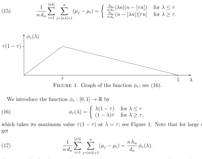
(15) 1 n dn [nλ] X i=1 n X j=[nλ]+1 (µj −µi) = hn n dn[λn](n−[τ n]) for λ≤τ hn n dn(n−[λn])[τ n] for λ≥τ. -6 XX XX XX XX XX XX XX XX XX XX XX XX XX τ(1−τ) τ 1 λ φτ(λ)
Figure 1. Graph of the function φτ; see (16).
We introduce the function φτ : [0,1]→R by
(16) φτ(λ) =
λ(1−τ) for λ≤τ
(1−λ)τ for λ≥τ,
which takes its maximum value τ(1−τ) at λ =τ; see Figure 1. Note that for large n, we get (17) 1 n dn [nλ] X i=1 n X j=[nλ]+1 (µj−µi)∼ n hn dn φτ(λ).
Thus, in order for the second term in (14) to converge as n → ∞, we have to choose the level shift hn ∼c dn/n. When n is large, this is exactly the order of the level shift that can
Theorem 2.1. Let (ξi)i≥1 be a stationary Gaussian process with mean zero, variance 1
and autocovariance function as in (4) with 0 < D < m1. Moreover, let G : R → R be a measurable function satisfying E(G2(ξ))< ∞ and define X
i = µi +G(ξi). Then under the
local alternative Aτ,hn(n) with
(18) hn∼
dn
n c,
for an arbitrary constantc, the process (Dn(λ))0≤λ≤1 in (14) converges in distribution to the
process (19) am m!(λZm(1)−Zm(λ)) +c φτ(λ) 0≤λ≤1 ,
where (Zm(λ))λ≥0 denotes the m-th order Hermite process with Hurst parameter H = 1−
Dm
2 ∈( 1
2,1), where am is given by (13) and φτ(λ) by (16).
Proof. We use the decomposition (14). The first term on the right hand side has the same distribution as Dn(λ) under the hypothesis, and thus converges in distribution to
am
m!(λZm(1)−Zm(λ)). Regarding the second term, we observe that by (18) and (15) we get
1 n dn [nλ] X i=1 n X j=[nλ]+1 (µj −µi) ∼ c n2[λn](n−[τ n]) for λ≤τ c n2(n−[λn])[τ n] for λ≥τ. → c φτ(λ), uniformly inλ ∈[0,1], as n → ∞.
Remark 2.2. (i) Observe that for c = 0 we recover the limit distribution under the null hypothesis. Thus, Theorem 2.1 is a generalization of the results obtained previously under the null hypothesis. The limit process is a fractional bridge process. When m = 1, this process is a fractional Gaussian bridge. For m >1, the process is non-Gaussian.
(ii) Under the local alternative, i.e. when c6= 0, the limit process is the sum of a fractional bridge process and the deterministic functionc φτ.
As an application of the continuous mapping theorem, we obtain the following corollary.
Corollary 2.3. Under the alternativeAτ,hn(n)withhn ∼
dn nc, Dn as defined in (7) converges in distribution to (20) sup 0≤λ≤1 am m!(λZm(1)−Zm(λ)) +c φτ(λ) .
Remark 2.4. (i) The limit distribution (20) depends on the constant c. For c = 0, we obtain the limit distribution under the null hypthesis. Quantiles of this limit distribution were calculated numerically via a Monte-Carlo simulation by Dehling, Rooch and Taqqu (2013), Table 1. Increasing the value of |c| leads to a shift of the distribution to the right. If c = ∞, that is, if hn tends slower to zero than dnnc for any c > 0, then the correct
normalization for Dn(λ) should go to ∞at a higher rate which would kill the random part
(λZm(1)−Zm(λ)) in (19), and hence the level shift could be detected precisely. The power
of the asymptotic test would be equal to 1 in this case.
(ii) For a given τ ∈ [0,1], the function φτ(λ) takes its maximum value in λ = τ, and this
maximum value equals τ(1−τ). Thus, for values of τ close to 0 and close to 1, τ(1−τ) is close to 0, and thus the effect of adding the term cφτ(λ) is rather small. As a result, the
power of the test is small at level shifts that occur very early or very late in the process. (iii) The higher the level shift and the closerλis to τ, the easier it is to detect the level shift.
(iv) If the observations are short-range dependent, one can typically detect level shifts hn of size √ n n = 1 √
n, but here, because of long-range dependence, the level shifts that can be
detected are of smaller order dn
n ∼
cn1−Dm/2L(n)
n =cn
−Dm/2L(n); note that Dm <1.
We will now apply Corollary 2.3 in order to make power calculations for the change-point test that rejects for large values of Dn. Under the null hypothesis of no level shift,
Dn D −→ sup 0≤λ≤1 |am| m! |λZm(1)−Zm(λ)|.
If we denote by qα the upper α-quantile of the distribution of sup0≤λ≤1|λZm(1)−Zm(λ)|,
we obtain lim n→∞PH Dn≥ |am| m! qα =P sup 0≤λ≤1 |am| m! |λZm(1)−Zm(λ)| ≥ |am| m! qα =α,
where PH indicates the probability under the null hypothesisH. Thus, the test that rejects
the null hypothesis H when Dn ≥
|am|
m! qα has asymptotic level α. If hn is chosen as in (18),
we obtain under the alternative Aτ,hn(n) (21) lim n→∞PAτ,hn(n) Dn≥ |am| m! qα =P sup 0≤λ≤1 am m!(λZm(1)−Zm(λ)) +c φτ(λ) ≥ |am| m! qα .
Thus, for large n, the power of our test at the alternative Aτ,hn(n) is approximately given by the right-hand side of (21).
We may also apply Corollary 2.3 in order to determine the size of a level shift at time [τ n] that can be detected with a given probability β. First, we calculate c=c(α, β) such that
(22) P sup 0≤λ≤1 am m!(λZm(1)−Zm(λ)) +c φτ(λ) ≥ |am| m! qα =β.
Thus, by (21), we get that the asymptotic power of the test at the alternative Aτ,hn(n) is equal toβ. Thus, given a sample size n, we can detect a level shift of size hn= dnnc(α, β) at
time [τ n] with probabilityβ with a level α test based on the test statisticDn.
3. Power of the Wilcoxon Change-Point Test under Local Alternatives
In the context of the Wilcoxon change-point test, the Hermite rank is not that of the function G, but of the class of functions
(23) 1{G(ξi)≤x}−F(x), x∈R,
where F(x) = E(1{G(ξi)≤x}) = P(G(ξi)≤ x). We define the Hermite expansion of the class of functions (23) as 1{G(ξi)≤x} −F(x) = ∞ X q=1 Jq(x) q! Hq(ξi),
where Hq is again the q-th order Hermite polynomial and where the coefficients are
(24) Jq(x) = E Hq(ξi)1{G(ξi)≤x}
.
We define the Hermite rank of the class of functions (23) as
Theorem 3.1. Suppose that (ξi)i≥1 is a stationary Gaussian process with mean zero,
vari-ance 1 and autocovariance function as in (4) with 0 ≤ D < m1. Moreover, let G : R → R
be a measurable function, and assume that G(ξk) has continuous distribution function F(x).
Let m denote the Hermite rank of the class of functions (23), let dn be as in (11), and let
the level shift hn be as in (18). Then, under the sequence of alternatives Aτ,hn, defined in (8), if hn →0 as n→ ∞, the process (25) 1 n dn [nλ] X i=1 n X j=[nλ]+1 1{Xi≤Xj}− 1 2 − n dn φτ(λ) Z R (F(x+hn)−F(x))dF(x) 0≤λ≤1
converges in distribution towards the process (26) R RJm(x)dF(x) m! Zm(λ)−λZm(1) 0≤λ≤1 ,
where (Zm(λ))λ≥0 denotes the m-th order Hermite process with Hurst parameter H = 1−
Dm
2 ∈( 1
2,1) and where Jm(x) is defined as in (24).
Remark 3.2. (i) The normalization dn and the processes (Zm(λ))λ≥0 in Theorem 2.1 and
Theorem 3.1 are the same.
(ii) Since, by assumption, the distributionF(x) ofG(ξk) is continuous, it follows from
integra-tion by parts thatR
RF(x)dF(x) = 1
2. This explains the 1/2 in (25) because
R
RF(x)dF(x) =
E(1{X1≤X10}), where X
0
1 is an independent copy of X1. The independence assumption is
rea-sonable as the dependence between Xi and Xj vanishes asymptotically when |i−j| → ∞.
(iii) As noted at the beginning of the proof, the first part of (25) converges to (26) under the null hypothesis. We show in the proof that the second part of (25) compensates for the presence of the alternatives Aτ,hn.
(iv) We make no assumption about the exact order of the sequence (hn)n≥1. Theorem 3.1
holds under the very general assumption that hn→0, as n → ∞.
(v) If we choose (hn)n≥1 as in (18), the centering constants in (25) converge, provided some
technical assumptions are satisfied. To see this, observe that
n dn φτ(λ) Z R (F(x+hn)−F(x))dF(x) ∼ n hn dn φτ(λ) Z R F(x+hn)−F(x) hn dF(x) → c φτ(λ) Z R f(x)dF(x) = c φτ(λ) Z R f2(x)dx.
The convergence in the next to last step requires some justification – this holds, e.g. if F is differentiable with bounded derivative f(x).
Corollary 3.3. Suppose that (ξi)i≥1 is a stationary Gaussian process with mean zero,
vari-ance 1 and autocovariance function as in (4) with0≤D < m1. Moreover, let G:R→R be a measurable function, and assume thatG(ξk) has a distribution functionF(x)with bounded
density f(x). Let m denote the Hermite rank of the class of functions 1{G(ξi)≤x} −F(x),
x ∈ R. Then, under the sequence of alternatives Aτ,hn, defined in (8), with hn ∼ c
dn n we obtain that (27) 1 n dn [nλ] X i=1 n X j=[nλ]+1 1{Xi≤Xj}− 1 2 0≤λ≤1
converges in distribution to the process R RJm(x)dF(x) m! (Zm(λ)−λZm(1)) +cφτ(λ) Z R f2(x)dx 0≤λ≤1 .
Proof of Theorem 3.1. In our proof, we will make use of the limit theorem that was derived in Dehling, Rooch and Taqqu (2013) under the null hypothesis. They showed (see Theorem 1) that (28) 1 n dn [nλ] X i=1 n X j=[nλ]+1 1{G(ξi)≤G(ξj)}− 1 2 → R RJm(x)dF(x) m! (Zm(λ)−λZm(1)).
In order to make use of this result, we will decompose the test statistic into a term whose distribution is the same both under the null hypothesis as well as under the alternative, and a second term which, after proper centering converges to zero. As in Dehling, Rooch and Taqqu (2013), we will express the test statistic as a functional of the empirical distribution function of the G(ξi), namely
Fk(x) = 1 k k X i=1 1{G(ξi)≤x}.
Given integersk, l withk ≤l we denote by Fk,l(x) the empirical distribution function based
onG(ξk), . . . , G(ξl), i.e. (29) Fk,l(x) = 1 l−k+ 1 l X i=k 1{G(ξi)≤x}. Recall that under the local alternative, we have
Xi =
G(ξi) +µ for i= 1, . . . ,[nτ]
G(ξi) +µ+hn for i= [nτ] + 1, . . . , n.
Thus, we obtain for λ≤τ,
[nλ] X i=1 n X j=[nλ]+1 1{Xi≤Xj} = [nλ] X i=1 [nτ] X j=[nλ]+1 1{G(ξi)+µ≤G(ξj)+µ}+ [nλ] X i=1 n X j=[nτ]+1 1{G(ξi)+µ≤G(ξj)+µ+hn} = [nλ] X i=1 [nτ] X j=[nλ]+1 1{G(ξi)≤G(ξj)} + [nλ] X i=1 n X j=[nτ]+1 1{G(ξi)≤G(ξj)+hn} = [nλ] X i=1 n X j=[nλ]+1 1{G(ξi)≤G(ξj)} + [nλ] X i=1 n X j=[nτ]+1 1{G(ξi)≤G(ξj)+hn}−1{G(ξi)≤G(ξj)} = [nλ] X i=1 n X j=[nλ]+1 1{G(ξi)≤G(ξj)} + [nλ] X i=1 n X j=[nτ]+1 1{G(ξj)<G(ξi)≤G(ξj)+hn}. (30)
In the same way, we obtain for λ≥τ, [nλ] X i=1 n X j=[nλ]+1 1{Xi≤Xj} = [nτ] X i=1 n X j=[nλ]+1 1{G(ξi)+µ≤G(ξj)+µ+hn}+ [nλ] X i=[nτ]+1 n X j=[nλ]+1 1{G(ξi)+µ+hn≤G(ξj)+µ+hn} = [nτ] X i=1 n X j=[nλ]+1 1{G(ξi)≤G(ξj)+hn}+ [nλ] X i=[nτ]+1 n X j=[nλ]+1 1{G(ξi)≤G(ξj)} = [nλ] X i=1 n X j=[nλ]+1 1{G(ξi)≤G(ξj)}+ [nτ] X i=1 n X j=[nλ]+1 1{G(ξi)≤G(ξj)+hn}−1{G(ξi)≤G(ξj)} = [nλ] X i=1 n X j=[nλ]+1 1{G(ξi)≤G(ξj)}+ [nτ] X i=1 n X j=[nλ]+1 1{G(ξj)<G(ξi)≤G(ξj)+hn} (31)
Thus, in order to prove Theorem 3.1, it suffices to show that the following two terms, (32) 1 n dn sup 0≤λ≤τ [nλ] X i=1 n X j=[nτ]+1 1{G(ξj)<G(ξi)≤G(ξj)+hn} −n 2λ(1−τ) Z R (F(x+hn)−F(x))dF(x) and (33) 1 n dn sup τ≤λ≤1 [nτ] X i=1 n X j=[nλ]+1 1{G(ξj)<G(ξi)≤G(ξj)+hn}−n 2τ(1−λ) Z R (F(x+hn)−F(x))dF(x)
both converge to zero in probability. We first show this for (32). Observe that
[nλ] X i=1 n X j=[nτ]+1 1{G(ξj)<G(ξi)≤G(ξj)+hn}−n 2λ(1−τ) Z R (F(x+hn)−F(x))dF(x) = [nλ] n X j=[nτ]+1 F[nλ](G(ξi) +hn)−F[nλ](G(ξi)) −n2λ(1−τ) Z R (F(x+hn)−F(x))dF(x) = [nλ](n−[nτ]) Z R F[nλ](x+hn)−F[nλ](x) dF[nτ]+1,n(x) −n2λ(1−τ) Z R (F(x+hn)−F(x))dF(x) = [nλ](n−[nτ]) Z R (F[nλ](x+hn)−F[nλ](x))dF[nτ]+1,n(x)− Z R (F(x+hn)−F(x))dF(x) + [nλ](n−[nτ])−n2λ(1−τ) Z R (F(x+hn)−F(x))dF(x)
Note that|[nλ](n−[nτ])−n2λ(1−τ)| ≤n and |R
R(F(x+hn)−F(x))dF(x)| ≤1. Thus 1 n dn [nλ](n−[nτ])−n2λ(1−τ) Z R (F(x+hn)−F(x))dF(x)≤ 1 dn →0,
as n → ∞. Hence, in order to show that (32) converges to zero in probability, it suffices to show that (34) 1 n dn [nλ](n−[nτ]) Z R (F[nλ](x+hn)−F[nλ](x))dF[nτ]+1,n(x)− Z R (F(x+hn)−F(x))dF(x)
converges to zero, in probability. In order to prove this, we rewrite the difference of the integrals in (34) as Z R F[nλ](x+hn)−F[nλ](x) dF[nτ]+1,n(x)− Z R (F(x+hn)−F(x))dF(x) (35) = Z R F[nλ](x+hn)−F[nλ](x) −(F(x+hn)−F(x))dF[nτ]+1,n(x) + Z R (F(x+hn)−F(x))d(F[nτ]+1,n−F)(x) = Z R F[nλ](x+hn)−F[nλ](x) −(F(x+hn)−F(x))dF[nτ]+1,n(x) − Z R F[nτ]+1,n(x)−F(x) d(F(x+hn)−F(x)),
where we have used integration by parts in the final step. Thus, in order to prove that (34) converges to zero, it suffices to show that the following two terms converge in probability, as
n→0, 1 dn [nλ] Z R (F[nλ](x+hn)−F[nλ](x))−(F(x+hn)−F(x)) dF[nτ]+1,n(x)→0 (36) 1 dn (n−[nτ]) Z R F[nτ]+1,n(x)−F(x) d(F(x+hn)−F(x))→0. (37)
In order to prove (36) and (37), we now apply the empirical process non-central limit theorem of Dehling and Taqqu (1989) which states that
d−n1[nλ](F[nλ](x)−F(x)) x∈[−∞,∞],λ∈[0,1] D −→(J(x)Z(λ))x∈[−∞,∞],λ∈[0,1], where J(x) =Jm(x) =E 1{G(ξi)≤x}Hm(ξi) and Z(λ) = Zm(λ) m! .
By the Dudley-Wichura version of Skorohod’s representation theorem (see Shorack and Well-ner (1986), Theorem 2.3.4) we may assume without loss of geWell-nerality that convergence holds almost surely with respect to the supremum norm on the function spaceD([0,1]×[−∞,∞]), i.e. (38) sup λ∈[0,1],x∈R d−n1[nλ](F[nλ](x)−F(x))−J(x)Z(λ) −→0 a.s.
Note that by definition, for any λ≤τ
([nτ]−[nλ])(F[nλ]+1,[nτ](x)−F(x)) = [nτ](F[nτ](x)−F(x))−[nλ](F[nλ](x)−F(x)).
Hence, we may deduce from (38) the following limit theorem for the empirical distribution of the observationsX[nλ]+1, . . . , X[nτ], (39) sup 0≤λ≤τ,x∈R d−n1([nτ]−[nλ])(F[nλ]+1,[nτ](x)−F(x))−J(x)(Z(τ)−Z(λ)) →0,
almost surely. In the same way, we obtain (40) sup 0≤λ≤1,x∈R d−n1(n−[nλ])(F[nλ]+1,n−F(x))−J(x)(Z(1)−Z(λ)) →0,
almost surely. Now we return to (36) and write
Z R 1 dn [nλ] (F[nλ](x+hn)−F[nλ](x))−(F(x+hn)−F(x)) dF[nτ]+1,n(x) (41) ≤ Z R (J(x+hn)−J(x))Z(λ)dF[nτ]+1,n(x) + sup x∈R,0≤λ≤1 1 dn [nλ] (F[nλ](x+hn)−F[nλ](x))−(F(x+hn)−F(x)) −(J(x+hn)−J(x))Z(λ) ≤ Z R (J(x+hn)−J(x))dF[nτ]+1,n(x) sup 0≤λ≤1 |Z(λ)| + sup x∈R,0≤λ≤1 1 dn [nλ] (F[nλ](x+hn)−F[nλ](x))−(F(x+hn)−F(x)) −(J(x+hn)−J(x))Z(λ) .
The second term on the right-hand side converges to zero by (38). Concerning the first term, note that (42) J(x) = Z R 1{G(y)≤x}Hm(y)φ(y)dy =− Z R 1{x≤G(y)}Hm(y)φ(y)dy, where φ(y) = √1 2πe −y2/2
denotes the standard normal density function. For the second identity, we have used the fact thatG(ξ), by assumption, has a continuous distribution, and that R
RHm(y)φ(y)dy= 0, for m≥1. Using (42) we thus obtain
Z R J(x)dF[nτ]+1,n(x) = − Z R Z R 1{x≤G(y)}Hm(y)φ(y)dydF[nτ]+1,n(x) (43) = − Z R Z R 1{x≤G(y)}dF[nτ]+1,n(x)Hm(y)φ(y)dy = − Z R F[nτ]+1,n(G(y))Hm(y)φ(y)dy,
and, using analogous arguments, (44) Z R J(x+hn)dF[nτ]+1,n(x) =− Z R F[nτ]+1,n(G(y)−hn)Hm(y)φ(y)dy.
By the Glivenko-Cantelli theorem, applied to the stationary, ergodic process (G(ξi))i≥1, we
get supx∈R|Fn(x)−F(x)| →0, almost surely. Since
F[nτ]+1,n(x) =
n
n−[nτ]Fn(x)−
[nτ]
n−[nτ]F[nτ](x), we get that, almost surely,
(45) sup x∈R F[nτ]+1,n(x)−F(x) →0.
Returning to the first term on the right-hand side of (41), we obtain, using (43) and (44), Z R (J(x+hn)−J(x))dF[nτ]+1,n(x) = Z R F[nτ]+1,n(G(y)−hn)−F[nτ]+1,n(G(y)) Hm(y)φ(y)dy ≤ Z R |F(G(y)−hn)−F(G(y))| |Hm(y)|φ(y)dy +2 sup x F[nτ]+1,n(x)−F(x) Z R |Hm(y)|φ(y)dy.
Both terms on the right-hand-side converge to zero; the second one by (45), the first one by continuity of F, the fact that hn → 0, and Lebesgue’s dominated convergence theorem. In
both cases, we have made use of the fact that R |Hm(y)|φ(y)dy <∞. Thus we have finally
established (36). In order to prove (37), we observe that 1 dn (n−[nτ]) Z R F[nτ]+1,n(x)−F(x) d(F(x+hn)−F(x)) ≤ Z R J(x)(Z(τ)−Z(1))d(F(x+hn)−F(x)) + sup x∈R 1 dn (n−[nτ])(F[nτ]+1,n(x)−F(x))−J(x)(Z(τ)−Z(1)) ≤ Z R J(x)d(F(x+hn)−F(x)) |Z(τ)−Z(1)| + sup x∈R 1 dn (n−[nτ])(F[nτ]+1,n(x)−F(x))−J(x)(Z(τ)−Z(1)) .
The second term on the right-hand side converges to zero, by (40). Concerning the first term, note that
Z
R
J(x)d(F(x+hn)−F(x)) = E(J(G(ξi)−hn)−J(G(ξi))).
Applying Lebesgue’s dominated convergence theorem and making use of the fact that, by assumption, J is continuous, we obtain that R
RJ(x)d(F(x+hn)−F(x))→0. In this way,
we have finally proved that (32) converges to zero, in probability. By similar arguments, we can prove this for (33), which finally ends the proof of Theorem 3.1.
4. ARE of the Wilcoxon Change-Point Test and the CUSUM Test for LRD
Data
In this section, we calculate the asymptotic relative efficiency (ARE) of the Wilcoxon change-point test with respect to the CUSUM test. To do so, we calculate the number of observations needed to detect a small level shift h at time [τ n] with a test of given level
α and given power β, both for the Wilcoxon change-point test and the CUSUM test, and denote these numbers by nW and nC, respectively. We then define the asymptotic relative
efficiency of the Wilcoxon change-point test with respect to the CUSUM test by
(46) ARE(W, C) = lim
h→0
nC
nW
.
It will turn out that the limit (46) exists and that the asymptotic relative efficiency does not depend on the choice of τ, α, β. If this limit is larger than 1, then the CUSUM test requires
a larger sample size to detect the level shift, and hence the Wilcoxon change-point test is (asymptotically) more efficient.
In the remaining part of this section, we will focus on the case when m = 1 both for the CUSUM as well as the Wilcoxon change-point test, i.e. when the Hermite rank ofG(ξ1) and
of the class of functions 1{G(ξ1)≤x} −F(x), x ∈ R, are both equal to 1. This is the case, for example, whenG is a strictly monotone function. In this case
Z
R
J1(x)dF(x) =−
1 2√π,
see Relation (20) in Dehling, Rooch and Taqqu (2013), showing that the Hermite rank of the class of functions 1{G(ξ1)≤x} −F(x), x ∈ R equals 1. Focusing now on G(ξ1) and using integration by parts, we get that the first order Hermite coefficient a1 of G equals
a1 =E(G(ξ1)ξ1) = Z R G(x)xφ(x)dx=− Z R G(x)φ0(x)dx = Z R φ(x)dG(x)>0, where φ(x) = √1 2πe −x2/2
denotes the standard normal density function. Thus, the Hermite rank ofG(ξi) equals 1, as well.
In this case, i.e. when m = 1, the Hermite process arising as limit in Theorem 2.1, Theorem 3.1 and Corollary 3.3 is fractional Brownian motion (BH(λ))0≤λ≤1. Note that
fractional Brownian motion is symmetric, i.e. (−BH(λ))0≤λ≤1 has the same distribution as
(BH(λ))0≤λ≤1. Thus the limit processes in Theorem 2.1 and Corollary 3.1 can also be written
as (47) (|a1|(BH(λ)−λBH(1)) +c φτ(λ))0≤λ≤1, (48) Z R J1(x)dF(x) (BH(λ)−λBH(1)) +c φτ(λ) Z R f2(x)dx 0≤λ≤1 .
As preparation, we first calculate a quantity that is related to the asymptotic relative efficiency, namely the ratio of the sizes of level shifts that can be detected by the two tests, based on the same number of observationsn, again for given values ofτ, α, β. We denote the corresponding level shifts by hW(n) and hC(n), respectively, assuming that these numbers
depend on n in the following way:
hW(n) = cW dn n (49) hC(n) = cC dn n. (50)
In order to simplify the following considerations, we take a one-sided change-point test, thus rejecting the hypothesis of no change-point for large values of
max 1≤k≤n−1 k X i=1 n X j=k+1 (Xj −Xi) or max 1≤k≤n−1 k X i=1 n X j=k+1 1{Xi≤Xj},
respectively. These are the appropriate tests when testing against the alternative of a non-negative level shift. In order to obtain tests that have asymptotically level α, the CUSUM
test and the Wilcoxon change-point test reject the null-hypothesis when 1 n dn|a1| max 1≤k≤n−1 k X i=1 n X j=k+1 (Xj −Xi)≥qα, (51) 1 n dn| R RJ1(x)dF(x)| max k=1,...,n−1 k X i=1 n X j=k+1 1{Xi≤Xj}− 1 2 ≥qα, (52)
where qα denotes the upper α quantile of the distribution of sup0≤λ≤1(BH(λ)−λBH(1)).
This follows from Theorem 2.1 and Corollary 3.3 after applying the continuous mapping theorem. The constantsa1 and the functionsJ1(x) are defined in (13) and (24), respectively,
and have just been computed. Under the sequence of alternatives Aτ,hC(n), the asymptotic distribution of the test statistic in (51) is given by
sup 0≤λ≤1 BH(λ)−λBH(1) + cC |a1| φτ(λ) ;
see Theorem 2.1. Under the sequence of alternatives Aτ,hW(n), the asymptotic distribution of the test statistic in (52) is given by
sup 0≤λ≤1 BH(λ)−λBH(1) + cW R Rf 2(x)dx |R RJ1(x)dF(x)| φτ(λ) ;
see Corollary 3.3. Thus, the asymptotic power of the CUSUM test is given by lim n→∞PAτ,hC(n) 1 n dn|a1| max 1≤k≤n−1 k X i=1 n X j=k+1 (Xj−Xi)≥qα ! =P sup 0≤λ≤1 BH(λ)−λBH(1) + cC |a1| φτ(λ) ≥qα . (53)
In the same way, we obtain the power of the Wilcoxon change-point test lim n→∞PAτ,hW(n) 1 n dn| R RJ1(x)dF(x)| max 1≤k≤n−1 k X i=1 n X j=k+1 1{Xi≤Xj}− 1 2 ≥qα ! =P sup 0≤λ≤1 BH(λ)−λBH(1) + cW R Rf 2(x)dx |R RJ1(x)dF(x)| φτ(λ) ≥qα . (54)
Thus, if we want the two tests to have identical power, we have to choose cC and cW in such
a way that cC |a1| φτ(λ) = cW R Rf 2(x)dx |R RJ1(x)dF(x)| φτ(λ),
which again yields by (49) and (50),
(55) hC(n) hW(n) = cC cW = |a1| R Rf 2(x)dx |R RJ1(x)dF(x)| .
This quantity gives the ratio of the height of a level shift that can be detected by a CUSUM test over the height that can be detected by a Wilcoxon change-point test, when both tests are assumed to have the same level α, the same power β and the shifts are taking place at the same time [nτ]. In addition, we assume that the tests are based on the same number of observations n, which is supposed to be large.
Example 4.1. In the case of Gaussian data, i.e. when G(ξ) = ξ, we have m = 1, a1 = E(ξ1H1(ξ1)) =E(ξ12) = 1, R Rf 2(x)dx =R R 1 2πe −x2 dx = 2√1 π and R RJ1(x)dF(x) =− 1 2√π; see
Dehling, Rooch and Taqqu (2013), Relation (20). Thus we obtain
(56) cC cW = 1/2 √ π 1/2√π = 1.
Hence, both tests can asymptotically, as n→ ∞, detect level shifts of the same height. The level shifts can be expressed in terms of
ψ(t) := P sup 0≤λ≤1 (BH(λ)−λBH(1) +t φτ(λ))≥qα ,
viewed as a function of t, for fixed values of τ and α. The function ψ is monotonically increasing. We define the generalized inverse,
ψ−(β) := inf{t≥0 :ψ(t)≥β}. Thus, we get (57) P sup 0≤λ≤1 BH(λ)−λBH(1) +ψ−(β)φτ(λ) ≥qα ≥β,
and, in fact, for given τ, α and β, ψ−(β) is the smallest number having this property. We can now apply Theorem 2.1 and Theorem 3.1. By comparing (53) and (57), we can detect a level shift of size h at time [nτ] with a CUSUM test of level α and power β based on n observations, if hC(n) ∼ dnncC, where cC satisfies |caC1| =ψ−(β). Hence we obtain that
hC(n) has to satisfy hC(n) = dn n |a1|ψ − (β) = n−D/2L(n)|a1|ψ−(β).
Similarly, by comparing (54) and (57), we get for the Wilcoxon change-point test that n has to satisfy hW(n) = n−D/2L(n) |R RJ1(x)dF(x)| R Rf 2(x)dx ψ −(β).
In the following theorem, we compute the asymptotic relative efficiency of the Wilcoxon change point test with respect to the CUSUM test.
Theorem 4.2. Let (ξi)i≥1 be a stationary Gaussian process with mean zero, variance 1
and autocovariance function as in (4). Moreover, let G : R → R be a measurable function satisfyingE(G2(ξ
1))<∞, and such thatG(ξ1)has a distribution functionF(x)with bounded
densityf(x). Assume that the Hermite rank ofG(ξ1)as well as the Hermite rank of the class
of functions (1{G(ξ1)≤x} −F(x)), x ∈ R are equal to 1. Moreover assume that 0 < D < 1. Then (58) ARE(TW, TC) = |a 1| R Rf 2(x)dx |R RJ1(x)dF(x)| 2/D ,
where TC and TW denote the CUSUM test and the Wilcoxon change-point test, respectively.
Proof. For abbreviation, we define
(59) b= |R RJ1(x)dF(x)| |a1| R Rf 2(x)dx 2/D .
We will show that the Wilcoxon change-point test based on b n observations has asymptot-ically the same power as the CUSUM test based on n observations. We will consider the local alternative
(60) ACn =Aτ,hC
n =Aτ,cdnn (n) for the CUSUM test, and the local alternative
(61) AWn =Aτ,hW
n =Aτ,cnbdn/b(n)
for the Wilcoxon change-point test. Note that under AWbn the level shift is the same as under
ACn. Further observe that, by (11),
hWn ∼c b ndn/b = c b nκ 1/2 1 (n/b)1 −D/2L1/2(n/b) = c b nκ 1/2 1 n 1−D/2 L1/2(n)bD/2−1L 1/2(n/b) L1/2(n) = cdn nb D/2 L(n/b) L(n) 1/2 ∼ cdn nb D/2 , (62)
where we have used the fact that L(n) is a slowly varying function.
For the CUSUM test, we can apply Corollary 2.3 and we obtain under the local alternative
AC n, that 1 |a1| Dn D −→ sup 0≤λ≤1 {(BH(λ)−λBH(1)) + 1 |a1| cφτ(λ)}.
For the Wilcoxon change-point test, we apply Corollary 3.3 with c replaced by c bD/2, in
view of (62). We thus obtain under the local alternative AW n , 1 |R RJ1(x)dF(x)| Wn D −→ sup 0≤λ≤1 (BH(λ)−λBH(1)) + R Rf 2(x)dx |R RJ1(x)dF(x)| c bD/2φτ(λ) = sup 0≤λ≤1 (BH(λ)−λBH(1)) + 1 |a1| c φτ(λ) ,
by (62). Letqαdenote the upperα-quantile of the distribution of sup0≤λ≤1{BH(λ)−λBH(1)};
then the test that rejects the null hypothesis when |a1
1|Dn ≥qαor when
1
|R
RJ1(x)dF(x)|
Wn ≥qα,
respectively, have asymptotically level α. The power of these tests at the alternatives AC n and AW n , respectively, converges to P sup 0≤λ≤1 (BH(λ)−λBH(1)) + 1 |a1| c φτ(λ) ≥qα .
Note that this also holds for the power along any other sequence, such asbn. Since the level shift at the alternative AC
n equals the level shift at the alternative AWbn, we have shown that
the Wilcoxon change-point test requires b n observations to yield the same performance as the CUSUM test with n observations. ThusARE(TW, TC) = 1/b, proving the theorem.
5. ARE of the Wilcoxon Change-Point Test and the CUSUM Test for IID
Data
We have shown in Example 4.1 that in the case of LRD data, the ARE of the Wilcoxon change-point test and the CUSUM test is 1 for Gaussian data. In this section, we will
compare this surprising result with the case of i.i.d. Gaussian data. We will find that in this case, the ARE is π3, i.e. the Wilcoxon change-point test is less efficient than the CUSUM test.
We consider i.i.d. observations X1, . . . , Xn with Xi ∼ N(0,1) and the U-statistic
Uk = k X i=1 n X j=k+1 h(Xi, Xj).
As kernel we will choose hC(x, y) = y−x and hW(x, y) = I{x≤y} − 12, in other words we
consider Uk(C) = k X i=1 n X j=k+1 hC(Xi, Xj) = k X i=1 n X j=k+1 (Xj−Xi), Uk(W) = k X i=1 n X j=k+1 hW(Xi, Xj) = k X i=1 n X j=k+1 I{Xi≤Xj}− 1 2 .
Both kernels hC, hW are antisymmetric, i.e. they satisfy h(x, y) = −h(y, x), so in order to
determine the limit behaviour ofUk(C) and Uk(W), we can apply the limit theorems of Cs¨org˝o and Horv´ath (1988).
Theorem 5.1. Let X1, . . . , Xn be i.i.d. random variables withXi ∼ N(0,1). Under the null
hypothesis of no change in the mean, one has sup 0≤λ≤1 1 n3/2U (C) [λn]−BB1,n(λ) =oP(1) (63) and sup 0≤λ≤1 1 n3/2q1 12 U[(λnW])−BB2,n(λ) =oP(1), (64)
where(BBi,n(λ))0≤λ≤1, i= 1,2, is a sequence of Brownian bridges with meanE[BBi,n(λ)] = 0
and auto-covariance E[BBi,n(s)BBi,n(t)] = min(s, t)−st.
Proof. By Theorem 4.1 of Cs¨org˝o and Horv´ath (1988), it holds under the null hypothesisH
that sup 0≤λ≤1 1 n3/2σU[λn]−BBn(λ) =oP(1)
where (BBn(λ))0≤λ≤1 is a sequence of Brownian bridges likeBB1,nandBB2,n above and where
σ2 =E[˜h2(X
1)] with ˜h(t) = E[h(t, X1)]. The kernelhhas to fulfillE[h2(X1, X2)]<∞which
is the case for hC(x, y) =y−x and hW(x, y) =I{x≤y}− 12 and GaussianXi.
Theorem 5.2. Let X1, . . . , Xn be i.i.d. random variables with Xi ∼ N(0,1). Under the
sequence of alternatives Aτ,hn(n) and with hn=
1
√
nc, where c is a constant, one has
1 n3/2U (C) [λn] 0≤λ≤1 →(BB1(λ) +cφτ(λ))0≤λ≤1 (65) and 1 n3/2q1 12 U[(λnW]) 0≤λ≤1 → BB2(λ) + c 2√π·q1 12 φτ(λ) 0≤λ≤1 (66)
in distribution, where (BBi(λ))0≤λ≤1 is a Brownian bridge, i= 1,2.
Proof. First, we prove (65). Like for the case of LRD observations, we decompose the statistic, so that we obtain under the sequence of alternatives Aτ,hn(n)
1 n3/2U (C) [λn] = 1 n3/2 [λn] X i=1 n X j=[λn]+1 (j −i) + 1 n3/2 [λn] X i=1 n X j=[λn]+1 (µj −µi).
By Theorem 5.1, the first term on the right-hand side converges to a Brownian bridgeBB(λ). For the second term we have like in the proof for LRD observations
1 n3/2 [λn] X i=1 n X j=[λn]+1 (µj−µi)∼ √ nhnφτ(λ),
and in order for the right-hand side to converge, we have to choose
(67) hn =
1
√
nc.
Now let us prove (66). Again like for LRD observations, we decompose the statistic into one term that converges like under the null hypothesis and one term which converges to a con-stant. Under the sequence of alternativesAτ,hn(n) and for the caseλ≤τ, this decomposition is (68) 1 n3/2U (W) [λn] = 1 n3/2 [λn] X i=1 n X j=[λn]+1 I{i≤j}− 1 2 + 1 n3/2 [λn] X i=1 n X j=[τ n]+1 I{j<i≤j+hn}. The first term converges uniformly to a Brownian Bridge, like under the null hypothesis. We will show that, if the observations i =G(ξi) are i.i.d. with c.d.f. F which has two bounded
derivatives F0 = f and F00, the second term converges uniformly to cλ(1−τ)R
Rf
2(x)dx,
which is cφτ(λ)
R
Rf
2(x)dx for the case λ≤τ. In the case of standard normally distributed
G(ξi), i.e. for F = Φ and f = ϕ, this function is c(2
√
π)−1φ
τ(λ). To this end, we consider
the following sequence of Hoeffding decompositions for the sequence of kernels hn(x, y) =
I{y<x≤y+hn}:
(69) hn(x, y) =ϑn+h1,n(x) +h2,n(y) +h3,n(x, y)
LetX, Y ∼F be i.i.d. random variables. Then we define
ϑn :=E[hn(X, Y)] = P(Y ≤X ≤Y +hn) = Z R Z y+hn y f(x)dx f(y)dy = Z R (F(y+hn)−F(y))f(y)dy = hn Z R F(y+hn)−F(y) hn f(y)dy ∼ hn Z R f2(y)dy, (70)
where in the last step we have used that (F(y+hn)−F(y))/hn→f(y) and the dominated
convergence theorem. Moreover, we set
h1,n(x) :=E[hn(x, Y)]−ϑn = E[I{Y <x≤Y+hn}]−ϑn = F(x)−F(x−hn)−ϑn
and h2,n(y) := E[hn(X, y)]−ϑn = E[I{y<X≤y+hn}]−ϑn = F(y+hn)−F(y)−ϑn and h3,n(x, y) := hn(x, y)−h1,n(x)−h2,n(y)−ϑn = I{y<x≤y+hn}−F(x) +F(x−hn) +ϑn−F(y+hn) +F(y). We will now show that
(72) sup 0≤λ≤τ 1 n3/2 [λn] X i=1 n X j=[τ n]+1 (h1,n(i) +h2,n(j) +h3,n(i, j)) →0
in probability, and from this it follows by the sequence of Hoeffding decompositions (69) that
sup 0≤λ≤τ 1 n3/2 [λn] X i=1 n X j=[τ n]+1 (hn(i, j)−ϑn) →0
i.e. that the second term in (68) converges uniformly to lim n→∞ 1 n3/2 [λn] X i=1 n X j=[τ n]+1 θn= lim n→∞ 1 n3/2[λn](n−[τ n])ϑn =λ(1−τ)c Z R f2(x)dx by (70) and (67).
We use the triangle inequality and show the uniform convergence to 0 for each of the three terms in (72) seperately. Since the parameter λ occurs only in the floor function value [λn], the supremum is in fact a maximum, and the h1,n(i) are i.i.d. random variables, so we can
use Kolmogorov’s inequality. We obtain for the first term in (72)
(73) P sup 0≤λ≤τ n−[τ n] n3/2 [λn] X i=1 h1,n(i) > s ≤ 1 s2 n2(1−τ)2 n3 [τ n] X i=1 Var[h1,n(i)].
Now consider an independent copy of the i and the Taylor expansion of F around the
value of, F(+hn) =F() +F0()hn+ F00(+δ) 2 h 2 n,
where the last term is the Lagrange remainder and thus+δ is between and +hn. Then
we obtain 1 h2 n Var[h1,n()] = Var F()−F(−hn) hn = Var f() +F00(+δ)hn 2 = Var [f()] + Var F00(+δ)hn 2 + 2 (E[f()F00(+δ)hn]−E[f()]E[F00(+δ)hn]),
and since f = F0 and F00 are bounded by assumption, we get Var[h1,n()] = O(h2n). Since
In the same manner, we obtain (74) P sup 0≤λ≤τ [λn] n3/2 n X j=[τ n]+1 h2,n(j) > s ≤ 1 s2 n2λ2 n3 n X j=1 Var[h2,n(j)]→0.
Finally, we have to show that
(75) sup 0≤λ≤τ 1 n3/2 [λn] X i=1 n X j=[τ n]+1 h3,n(i, j) →0
in probability. We set temporarily l := [λn] and T := [τ n] and obtain from Markov’s inequality P max 0≤l≤T 1 n3/2 l X i=1 n X j=T+1 h3,n(i, j) > s ! ≤ 1 s2E " max 0≤l≤T 1 n3/2 l X i=1 n X j=T+1 h3,n(i, j) #2 .
Now for any collection of random variablesY1, . . . , Yk, one hasE[max{Y12, . . . Yk2}]≤
Pk i=1EY 2 i , so that 1 s2E " max 0≤l≤T 1 n3/2 l X i=1 n X j=T+1 h3,n(i, j) #2 ≤ 1 s2 1 n3 T X l=1 E " l X i=1 n X j=T+1 h3,n(i, j) #2 = 1 s2 1 n3 T X l=1 l X i=1 n X j=T+1 Var [h3,n(i, j)],
where in the last step we have used that h3,n(i, j) are uncorrelated by Hoeffding’s
decom-position. Now for two i.i.d. random variables , η, we have, like above with the Taylor expansion of F: Var [h3,n(, η)] = Var I{η<≤η+hn}−F() +F(−hn) +ϑn−F(η+hn) +F(η) = VarI{η<≤η+hn}−hn(f() +OP(hn)) +hn(f(η) +OP(hn)) = VarI{η<≤η+hn} + Var [hn(f() +f(η) +OP(hn))] + 2CovI{η<≤η+hn}, hn(f() +f(η) +OP(hn)) ≤(ϑn−ϑ2n) +h 2 nO(1) + 2 p (ϑn−ϑ2n)·h2nO(1) =O(hn),
using (70). We have just shown that
P max 0≤l≤T 1 n3/2 l X i=1 n X j=T+1 h3,n(i, j) > s ! ≤ 1 s2O(hn),
which proves (75). So we have proven (68) for the case λ ≤ τ. The proof for λ > τ is
similar.
Now the stage is set to calculate the ARE of the Wilcoxon test based on U[(λnW]) and the CUSUM test based on U[(λnC)], as defined in the section about the ARE in the LRD case. Let
qα denote the upper α-quantile of the distribution of sup0≤λ≤1BB(λ). By Theorem 5.2, the
power of the tests is given respectively by
(76) P sup 0≤λ≤1 (BB(λ) +cCφτ(λ))≥qα
and (77) P sup 0≤λ≤1 BB(λ) +cW 1 σ·2√πφτ(λ) ≥qα
where σ2 = 1/12 and we assume that
hW(n) = cW √ n, hC(n) = cC √ n.
Thus if we want both tests to have identical power, we must ensure thatcC =cW/(σ·2
√ π), in other words hC(n) hW(n) = cC cW = 1 σ·2√π.
Now we define, as in the proof for LRD observations, the probability
ψ(t) :=P sup 0≤λ≤1 (BB(λ) +t φτ(λ))≥qα ,
for whose generalized inverseψ− holds
(78) P sup 0≤λ≤1 BB(λ) +ψ−(β)φτ(λ) ≥qα ≥β.
Now, comparing (78) and (76), we conclude that we can detect a level shift of sizeh at time [nτ] with the CUSUM test of (asymptotic) level α and powerβ based on n observations, if
hC(n) = √cCn and where cC satisfies cC =ψ−(β); hence we obtain that hC(n) has to satisfy
hC(n) = 1 √ nψ − (β).
In the same manner, we get for the Wilcoxon test the conditionshW(n) = √cWn andcW/(σ2
√ π) = ψ−(β) and thus hW(n) = σ2√π √ n ψ − (β).
Solving these two equations for n again and denoting the resulting numbers of observations bynC and nW, respectively, we obtain
nC = 1 hC ψ−(β) 2 nW = 2σ√π hW ψ−(β) 2 .
To obtainARE(TW, TC), we equatehW and hC. We then obtain the following theorem.
Theorem 5.3. Let X1, . . . , Xn be i.i.d. random variables with Xi ∼ N(0,1). Then
ARE(TW, TC) = lim h→0 nC nW = (2σ√π)−2 = 3 π, (79)
where TC, TW denote the one-sided CUSUM-test, respectively the one-sided Wilcoxon test,
6. Simulation Results
We have proven that for Gaussian data, the CUSUM test and the Wilcoxon change-point test show asymptotically the same performance, i.e. that their ARE is 1. For Pareto(3,1) distributed data, we obtain, using (58) and numerical integration, an ARE of approximately (2.68)2/D. Now we will illustrate these findings by a simulation study.
6.1. Gaussian data. We consider realizations ξ1, . . . , ξn of a fGn process with Hurst
pa-rameterH = 0.7 (D= 0.6), using the fArma package in R, and create observations
Xi =
(
G(ξi) for i= 1, . . . ,[nλ]
G(ξi) +h for i= [nλ] + 1, . . . , n
,
by applying a transformation G which is (with respect to the standard normal measure) normalized and square-integrable: E[G(ξ)] = 0, E[G2(ξ)] = 1 for ξ ∼ N(0,1). As a first
step, we choose G(t) = t in order to obtain Gaussian observations X1, . . . , Xn (later we
will choose a function G such that we obtain Pareto distributed data). In other words, we consider data which follow the local alternative
Aλ,h :
(
µ=E[Xi] = 0 fori= 1, . . . ,[nτ]
µ=E[Xi] =h fori= [nτ] + 1, . . . , n,
as in (8). In contrast to the simulations by Dehling, Rooch and Taqqu (2013), we choose a sample sizen= 2,000 instead ofn= 500. We let both the break point k= [τ n] and the level shift h:=µk+1−µk vary; specifically, we choose k = 100,200,600,1000 (which corresponds
to τ = 0.05,0.1,0.3,0,5) and we let h = 0.5,1,2. For each of these situations, we will compare the power of the CUSUM test and the power of the Wilcoxon change-point test in the test problem (H, Aλ,h): We have repeated each simulation 10,000 times and counted,
how often the respective test (correctly) rejected the null hypothesis.
Since our theoretical considerations yield an ARE of 1, we expect that both tests detect jumps equally well – that means that both tests, set on the same level, detect jumps of the same height and at the same position in the same number of observations with the same relative frequency. And indeed, we can clearly see in Table 1 that the power of both tests approximately coincides at many points; differences can be spotted only when the break occurs early in the data.
relative jump position τ
0.05 0.1 0.3 0.5
h=0.5 0.074 0.153 0.767 0.874
h=1 0.153 0.694 1.000 1.000
h=2 0.828 1.000 1.000 1.000
relative jump positionτ
0.05 0.1 0.3 0.5
h=0.5 0.072 0.143 0.765 0.876
h=1 0.128 0.602 1.000 1.000
h=2 0.321 1.000 1.000 1.000
Table 1. Power of the CUSUM test (left) and of the Wilcoxon change-point
test (right), for n = 2000 observations of fGn with LRD parameter H = 0.7, different break points [τ n] and different level shifts h. Both tests have asymptotically level 5%. The calculations are based on 10,000 simulation runs.
6.2. Heavy tailed data. We consider again realizations ξ1, . . . , ξn of a fGn process with
Hurst parameter H = 0.7 (D= 0.6) and create observations
Xi =
(
G(ξi) for i= 1, . . . ,[nλ]
G(ξi) +h for i= [nλ] + 1, . . . , n
,
by applying the transformation
G(t) = p1 3/4 (Φ(t))−1/3− 3 2 .
In this case, the first Hermite coefficient of G, obtained by numerical integration, equals
a1 ≈ −0.6784. This transformation G produces observations Xi = G(ξi) which follow
a standardized Pareto(3,1) distribution with mean zero and variance 1. The probability density function of Xi is given by
f(x) = 3 q 3 4 q 3 4x+ 3 2 −4 if x≥ −q1 3 0 else.
To the second sample of observations, X[τ n]+1, . . . , Xn, we again add a constant h, but this
time we choose
(80) h=hn=c
dn
n =cn
−D/2
as in (18). We let the break point k = [τ n] vary; here, we choose τ = 0.05,0.1,0.3,0.5. We let also the sample size vary; we will give details below. To these data, we have applied the CUSUM test and the Wilcoxon change-point test, and under 10,000 simulation runs we counted how often the respective test (rightly) rejected the null hypothesis.
Now our theoretical considerations, see (58), predict for this situation
ARE = lim n→∞ nC nW = |a 1| R Rf 2(x)dx |R RJ1(x)f(x)dx| 2/D ≈(2.67754)2/0.6 ≈26.655.
This means that the CUSUM test needs approximately 26.66 times as many observations as the Wilcoxon test in order to detect the same jump on the same level with the same probability. In order to find this behaviour, we have analysed the power of the Wilcoxon test for nW = 10,50,100,200 observations and the power of the CUSUM test for nC =
266,1332,2666,5330 observations.
In order to be able to compare the two tests, we need to have identical level shifts when applying the Wilcoxon test to a sample of size nW and the CUSUM test to a sample of
size nC = 26.655nW. This can be achieved by choosing the constants cin (80) accordingly,
namely taking cC = 2.67754cW. In this way, we obtain
hCn C =cCn −D/2 C = 2.67754cW(26.655nW)−D/2 =cWn −D/2 W =h W nW.
We ran simulations for two different choices of cW, namelycW = 1 and cW = 2; see Table 3
and Table 4 for the results.
Here, we have to face a problem which was already encountered by Dehling, Rooch and Taqqu (2013). For the heavy-tailed Pareto data, the convergence of the CUSUM test statistic towards its limit is so slow that the asymptotic quantiles of the limit distribution are not appropriate as critical values to define the domain of rejection of the test: In finite sample situations, the observed level of the test is not 5% – as it should be when using the 5%-quantile of the asymptotic limit distribution. In order to remedy this, we used as critical value for the test, the finite sample 5% quantiles of the distribution of the CUSUM test
statistic under the null hypothesis, using a Monte Carlo simulation; see Table 6 in Dehling, Rooch and Taqqu (2013). Here, we have performed the same steps, but for sample sizes
n=nC = 266,1332,2666,5330. The results are given in Table 2. Note that this problem does
not arise when using the Wilcoxon change-point test, since the Wilcoxon test is distribution free under the null hypothesis.
n 266 1332 2666 5330 ∞
qemp,0.05 0.73 0.66 0.64 0.63 0.59
Table 2. 5%-quantiles of the finite sample distribution of the CUSUM test
under the null hypothesis for Pareto(3,1)-transformed fGn with LRD param-eter H = 0.7 and different sample sizes n=nC.
The simulation results are shown in Table 3 (forcW = 1) and Table 4 (forcW = 2). Indeed,
for a fixed jump positionτ, the power of the CUSUM test (forn=nC = 266,1332,2666,5330
observations) and of the Wilcoxon test (forn=nW = 10,50,100,200 observations) coincide.
They are not fully equal, but we conjecture this is due to the small sample size which conflicts with the asymptotic character of our results. But it becomes clear: The CUSUM test needs quite a number of observations more to detect the same jump on the same level with the same probability – as predicted by our calculation around 25 times as many.
relative jump positionτ n h 0.05 0.1 0.3 0.5 266 0.50 0.049 0.049 0.066 0.088 1332 0.31 0.050 0.052 0.083 0.110 2666 0.25 0.052 0.055 0.092 0.127 5330 0.20 0.051 0.054 0.099 0.130
relative jump position τ n h 0.05 0.1 0.3 0.5 10 0.50 0.036 0.025 0.033 0.079 50 0.31 0.049 0.051 0.093 0.120 100 0.25 0.050 0.053 0.102 0.134 200 0.20 0.051 0.055 0.103 0.134
Table 3. Power of the CUSUM test (left) and of the Wilcoxon change-point
test (right), at different break points [τ n], different sample sizes n, and differ-ent jump heightsh, for Pareto(3,1) distributed data. Both tests have asymp-totically level 5% (CUSUM test is performed with empirical quantiles). The calculations are based on 10,000 simulation runs.
relative jump positionτ n h 0.05 0.1 0.3 0.5 266 1.00 0.049 0.054 0.162 0.259 1332 0.62 0.052 0.062 0.236 0.345 2666 0.50 0.055 0.069 0.272 0.390 5330 0.41 0.054 0.074 0.287 0.402
relative jump position τ n h 0.05 0.1 0.3 0.5 10 1.00 0.033 0.024 0.039 0.197 50 0.62 0.049 0.055 0.199 0.283 100 0.50 0.051 0.063 0.225 0.316 200 0.41 0.054 0.066 0.242 0.338
Table 4. Power of the CUSUM test (left) and of the Wilcoxon change-point
test (right) at different break points [τ n], different sample sizesn, and different jump heights h, for Pareto(3,1) distributed data. Both tests have asymptot-ically level 5% (CUSUM test is performed with empirical quantiles). The calculations are based on 10,000 simulation runs.
References
[1] Mikl´os Cs¨org˝o and Lajos Horv´ath (1988): Invariance Principle for Changepoint
Problems, Journal of Multivariate Analysis 27, 151–168.
[2] Mikl´os Cs¨org˝oandLajos Horv´ath(1997): Limit Theorems in Change-Point
Anal-ysis.J. Wiley & Sons, Chichester.
[3] Herold Dehling and Murad S. Taqqu (1989): The Empirical Process of Some
Long-Range Dependent Sequences with an Application to U-Statistics. The Annals of Statistics 17, 1767–1783.
[4] Herold Dehling, Aeneas Rooch and Murad S. Taqqu (2013): Nonparametric
Change-Point Tests for Long-Range Dependent Data.Scandinavian Journal of Statistics
40, 153–173.
[5] Vladas Pipiras and Murad S. Taqqu (2010): Regularization and Integral
Repre-sentations of Hermite Processes.Statistics and Probability Letters 80, 697–705.
[6] Galen R. Shorack and Jon A. Wellner (1986): Empirical Processes with
Appli-cations to Statistics.John Wiley & Sons, New York.
[7] Murad S. Taqqu (1979): Convergence of Integrated Processes of Arbitrary Hermite
Rank.Zeitschrift f¨ur Wahrscheinlichkeitstheorie und verwandte Gebiete 50, 53–83. Fakult¨at f¨ur Mathematik, Ruhr-Universit¨at Bochum, 44780 Bochum, Germany
E-mail address: [email protected]
Fakult¨at f¨ur Mathematik, Ruhr-Universit¨at Bochum, 44780 Bochum, Germany
E-mail address: [email protected]
Department of Mathematics, 111 Cummington St., Boston University, Boston MA 02215