Pixelor: A Competitive Sketching AI Agent. So you think you can
sketch?
AYAN KUMAR BHUNIA
∗,
SketchX, CVSSP, University of Surrey, UKAYAN DAS
∗,
SketchX, CVSSP, University of Surrey, iFlyTek-Surrey Joint Research Centre on Artificial Intelligence, UKUMAR RIAZ MUHAMMAD
∗,
SketchX, CVSSP, University of Surrey, UKYONGXIN YANG,
SketchX, CVSSP, University of Surrey, iFlyTek-Surrey Joint Research Centre on Artificial Intelligence, UKTIMOTHY M. HOSPEDALES,
University of Edinburgh, SketchX, CVSSP, University of Surrey, UKTAO XIANG,
SketchX, CVSSP, University of Surrey, iFlyTek-Surrey Joint Research Centre on Artificial Intelligence, UKYULIA GRYADITSKAYA,
SketchX, CVSSP, University of Surrey, iFlyTek-Surrey Joint Research Centre on Artificial Intelli-gence, UKYI-ZHE SONG,
SketchX, CVSSP, University of Surrey, iFlyTek-Surrey Joint Research Centre on Artificial Intelligence, UKPixelor
Human
(a) Early recognition (b) Multiple optimal strategies
Pixelor’s (AI) ‘Birthday cake’ sketch 1
Pixelor’s (AI) ‘Birthday cake’ sketch 2
Pixelor’s (AI) ‘Birthday cake’ sketch 3
Fig. 1. Our AI sketching agentPixelorlearns sketching strategies that lead to early sketch recognition. (a) In a competitive scenario,Pixelorand a human
player sketch a specified visual concept, while a judge (human or recognizer AI) attempts to recognize the concept. The competitor whose sketch is correctly recognized first is the winner. Winning requires conveying as much as possible with few pixels/little ink. (b) Trained on human sketches,Pixeloris able to learn multiplewinning sketching strategies.
We present the first competitive drawing agentPixelorthat exhibits human-level performance at a Pictionary-like sketching game, where the participant
∗
These authors contributed equally.
Authors’ addresses: Ayan Kumar Bhunia, [email protected], SketchX, CVSSP, University of Surrey, UK; Ayan Das, [email protected], SketchX, CVSSP, University of Surrey, iFlyTek-Surrey Joint Research Centre on Artificial Intelligence, UK; Umar Riaz Muhammad, [email protected], SketchX, CVSSP, University of Sur-rey, UK; Yongxin Yang, SketchX, CVSSP, University of SurSur-rey, iFlyTek-Surrey Joint Research Centre on Artificial Intelligence, UK, [email protected]; Timothy M. Hospedales, University of Edinburgh, SketchX, CVSSP, University of Surrey, UK, [email protected]; Tao Xiang, SketchX, CVSSP, University of Surrey, iFlyTek-Surrey Joint Research Centre on Artificial Intelligence, UK, [email protected]; Yulia Gryaditskaya, SketchX, CVSSP, University of Surrey, iFlyTek-Surrey Joint Research Centre on Artificial Intelligence, UK, [email protected]; Yi-Zhe Song, SketchX, CVSSP, University of Surrey, iFlyTek-Surrey Joint Research Centre on Artifi-cial Intelligence, UK, [email protected].
© 2020 Copyright held by the owner/author(s). Publication rights licensed to ACM. This is the author’s version of the work. It is posted here for your personal use. Not for redistribution. The definitive Version of Record was published inACM Transactions on
Graphics, https://doi.org/10.1145/3414685.3417840.
whose sketch is recognized first is a winner. Our AI agent can autonomously sketch a given visual concept, and achieve a recognizable rendition as quickly or faster than a human competitor. The key to victory for the agent’s goal is to learn the optimal stroke sequencing strategies that generate the most recognizable and distinguishable strokes first. TrainingPixeloris done in two steps. First, we infer the stroke order that maximizes early recognizability of human training sketches. Second, this order is used to supervise the training of a sequence-to-sequence stroke generator. Our key technical contributions are a tractable search of the exponential space of orderings using neural sorting; and an improved Seq2Seq Wasserstein (S2S-WAE) generator that uses an optimal-transport loss to accommodate the multi-modal nature of the optimal stroke distribution. Our analysis shows thatPixeloris better than the human players of theQuick, Draw!game, under both AI and human judging of early recognition. To analyze the impact of human competitors’ strategies, we conducted a further human study with participants being given unlimited thinking time and training in early recognizability by feedback from an AI judge. The study shows that humans do gradually improve their strategies with training, but overallPixelorstill matches human performance. The code and the dataset are available at http://sketchx.ai/pixelor.
CCS Concepts: •Computing methodologies→Search methodologies; Machine learning algorithms;Image manipulation;Modeling and simulation. Additional Key Words and Phrases: Sketch-generation, neural search, early recognition, AI games, recurrent neural network
ACM Reference Format:
Ayan Kumar Bhunia, Ayan Das, Umar Riaz Muhammad, Yongxin Yang, Timothy M. Hospedales, Tao Xiang, Yulia Gryaditskaya, and Yi-Zhe Song. 2020. Pixelor: A Competitive Sketching AI Agent. So you think you can sketch?.ACM Trans. Graph.39, 6, Article 166 (December 2020), 15 pages. https://doi.org/10.1145/3414685.3417840
1 INTRODUCTION
The majority of sketch research to date has focused on making sense
of existing human sketch data, including the problems of sketch
recognition [Eitz et al. 2012; Schneider and Tuytelaars 2014; Yu
et al. 2017], segmentation [Schneider and Tuytelaars 2016; Yang
et al. 2020], beautification [Bessmeltsev and Solomon 2019;
Simo-Serra et al. 2018] and 3D inference [Su et al. 2018; Xu et al. 2014].
Others have also explored the relationship between sketch and
photo via the practical application of sketch-based image retrieval
[Sangkloy et al. 2016; Yu et al. 2016]. Instead of just learning a
sketch-specific feature representation, these works aim to learn a
joint embedding between photo and sketch where retrieval can be
conducted. Sketches are the result of a dynamic drawing process –
they can be highly abstract and subject to individual drawing skill
variability – are thus distinctively different to photos: photos are
static and pixel-perfect visual representations.
While static sketch generation and stylization given a photo or
an image [Berger et al. 2013; Li et al. 2019; Liu et al. 2020] were
studied in vision and graphics communities for a long while, only
recently were we able to train machines to draw novel sketches [Ha
and Eck 2018]. This task is of fundamental importance to visual
understanding of sketches – the AI agent needs to mimic the actual
human drawing process stroke-by-stroke to produce a plausible
sketch, accommodating different style and abstraction levels
(Fig-ure 1). We aim to push the envelope further by introducing an agent
that not only can sketch like a human, but also does so with a stroke
sequence targeted at early recognizable rendition – just as a good
human Pictionary player would do!
In conventional Pictionary, a human player draws an object while
being continually evaluated by another human judge. The score in
the game depends on how quickly the judge guesses the player’s
intended object. To train an optimal drawing strategy, we need
a training set that is representative of strategies used by strong
players. We conduct a study on QuickDraw [Ha and Eck 2018], the
largest human sketch dataset to date. We found that albeit with
different styles and levels of abstraction, stroke drawing order is a
dominant factor in winning the game. For sketches drawn under
the time-pressured condition of QuickDraw data collection, human
stroke ordering is dramatically better than random: confirming the
existence and exploitation by participants of a mental model of
stroke informativeness. A key discovery is that the most common
ordering is not the optimal one needed to win a Pictionary game,
and moreover the few good winning Pictionary players exploit dis-tinctstroke orderings. That is, the distribution of optimally ordered
sketches with an early recognition property is multi-modal (Figures
1b, 5 and 6).
We trainPixelor, our competitive sketching agent, with a two-stage framework. The first two-stage inputs a given set of training
sketches with arbitrary sequential ordering and infers the stroke-levelordering that maximizes early recognition for this train set, which is typically better than the human ordering in the raw
in-put. To infer the target stroke ordering we exploit Sketch-a-Net
2.0 [Yu et al. 2017] to score the recognizability of a partial sketch.
An obvious strategy is to exhaustively evaluate all possible stroke
orders, however, such exhaustive search results in a computationally
intractable combinatorial search space. As a tractable optimization
strategy over strokes permutations, we leverageNeuralSort[Grover et al. 2019], a continuous relaxation of a classical sorting algorithm
that allows backward flow of straight-through (ST) gradients
[Ben-gio et al. 2013]. Existing applications of differentiable sorting have
used hand-crafted losses [Cuturi et al. 2019; Grover et al. 2019],
instead we deploy it to optimize a learnedperceptualloss [ John-son et al. 2016] in the form of Sketch-a-Net recognition accuracy.
Overall, this framework side-steps combinatorial search of stroke
ordering by learning a stroke scoring function, such that sorting
strokes by score achieves early recognition.
In the second stage, we use the optimal training set computed
above to train a Seq2Seq Wasserstein autoencoder (S2S-WAE) sketch
generation agent. Classic stroke-based sketch generators [Ha and
Eck 2018] are based on the standard Kullback-Leibler (KL)
diver-gence loss widely used in variational autoencoders [Bowman et al.
2016; Kingma and Welling 2014]. Our contribution is to replace this
with an optimal transport induced loss [Tolstikhin et al. 2018]. This
design choice is necessitated by observations made in the
afore-mentioned human study – the stroke ordering maximizing early
recognition is inherently a multi-modal distribution that is better
captured using the Wasserstein autoencoder [Tolstikhin et al. 2018].
In addition, we use a Transformer encoder [Vaswani et al. 2017] in
order to capture better contextual information compared to
bidirec-tional LSTM in our sketch generator.
To evaluatePixelor, we compare its generated sketches with those
from human participants in theQuick, Draw! game in terms of
early recognizability. We find that for both AI Sketch-a-Net and
human judging,Pixelorsketches are recognized earlier than the Quick, Draw!sketches that form its training data – thus confirming the impact of our stroke order learning. To understand the impact
of human sketching conditions on early recognition performance,
we conduct a new human study by collecting new sketches via a
custom-built on-line interface. In this study humans are instructed
to optimize their stroke order for early recognition and given
on-the-fly feedback on recognizability in the form of accuracy of the
AI classifier. Our analysis shows that with such training, humans
do gradually improve their performance in terms of early sketch
recognizability. Crucially, (and unlike inQuick, Draw!), humans are given unlimited time to think about their sketch. We compare
AI and human sketches with pixel-level synchronization, without
penalizing clock time or physical drawing speed. The results show
thatPixelortrained on old (but reordered)Quick, Draw!data still matches human performance under these challenging conditions.
As an application of this work, we define a competitive
AI-vs-human sketching game termed Pixelary, where a AI-vs-human competes
with a pixel-synchronizedPixeloragent to draw an object that can be recognized more quickly by an AI judge.
The main contributions of our work can be summarized as:
• We presentPixelor: The first competitive sketching agent that produces novel renditions of a given concept with early
recognizability.
• We generate training data forPixelorby solving for the stroke order that maximizes early recognition. We formulate this
problem as anoptimization over strokes permutationsand utilize a differentiable solver to learn a stroke scoring model
end-to-end. The trained model can be used to compute the
optimal order of any given sketch.
• Our sketching agentPixeloris implemented by a Sequence-to-Sequence Wasserstein Auto-Encoder with
transformer-encoder to handle the multi-modeal distribution of optimal
strategies present in the sketches of good Pictionary players.
• We conduct a comprehensive study using both automated
and human evaluation to demonstrate the efficacy of our
agent. The results show thatPixelorsurpasses human perfor-mance as exhibited in theQuick, Draw!game, and matches the human performance exhibited in our new study with more
favorable conditions and training for the human competitors.
2 RELATED WORK
Sketch synthesis.Most existing sketch synthesis models take raster image as input and follow a photo-to-sketch synthesis paradigm
where the task is to produce a human sketch styled version of the
input photo. Early works either rely on training a category-specific
pictorial structure model [Li et al. 2017] or visual abstraction model
[Berger et al. 2013] that replaces strokes from photo edge maps with
those of humans. Recent attempts were mostly motivated by neural
style transfer methods from the photo domain [Chen et al. 2017b;
Gatys et al. 2016; Johnson et al. 2016; Ulyanov et al. 2016]. Zhang
et al. [2017] integrated a residual U-net to apply painting styles to
sketches with an auxiliary classifier generative adversarial network
(AC-GAN) [Odena et al. 2017]. Another class of generative models
exists that learns to draw by means of model-free [Ganin et al. 2018]
or model-based [Huang et al. 2019] exploration. Such models exploit
reinforcement learning algorithms to incorporate immediate
feed-back from a drawing environment. However, such approaches are
known to be sample-inefficient and hence hard to train. Although,
recent works [Zheng et al. 2018] tried to alleviate this drawback to
some extent by learning differentiable environment models [Ha and
Schmidhuber 2018].
Ha and Eck [2018] proposed SketchRNN, a sequence-to-sequence
variational autoencoder (Seq2Seq-VAE [Bowman et al. 2016]) to
model the sequential sketching process. In this model, the encoder
is a bi-directional recurrent neural network (RNN) that takes in
a vectorized human sketch and produces a Gaussian distribution
over a latent vector that summarizes the sketch, and the decoder is
an autoregressive RNN that samples an output sketch conditioned
on a random vector drawn from that distribution. The SketchRNN
model is trained to mimic the human sketching process including
both style and temporal order. Our desired competitive-sketching
agent however must furthermore generate sketches efficiently to
achieve early recognition with few strokes. To this end it must solve
additional challenges, highlighted by a comprehensive analysis on
human sketch data (Section 3). First, there are several potential
routes to a winning sketching strategy, so it must be able to
repre-sent multi-modal data. Second, winning strategies turn out to use
more jumps between the end-point and start-point of temporally
consecutive strokes than in typical human sketches. The above
men-tioned SketchRNN model struggles to represent such strategies and
generates non-optimal sketching sequences, even if trained with
optimally ordered data. To address this issue, we advance sketch
generation by employing an optimal transport induced loss for the
sequential generative model learning (instead of Kullback-Leibler
(KL) divergence loss used in [Bowman et al. 2016; Ha and Eck 2018]).
Sketch recognition.Early methods for sketch recognition were developed to deal with professionally drawn sketches as in CAD
or artistic drawings [ Jabal et al. 2009; Lu et al. 2005; Sousa and
Fonseca 2009]. A more challenging task of free-hand sketch
recog-nition was first tackled in [Eitz et al. 2012] along with the release
of the first large-scale dataset of amateur sketches. Initial attempts
[Li et al. 2015; Schneider and Tuytelaars 2014] to solve this
prob-lem consisted mainly of using hand-crafted features together with
classifiers such as SVM. Inspired by the success of deep
convolu-tional neural networks (CNN) on various image related problems,
the first CNN-based sketch recognition model was proposed in [Yu
et al. 2015]. This outperformed previous hand-crafted features, and
was followed by various subsequent CNN-based approaches [Jia
et al. 2017; Sarvadevabhatla et al. 2018; Yu et al. 2017]. In this paper,
we ask a more challenging question – instead of asking AI to
rec-ognize pre-drawn sketches, can we train agents to draw sketches
from scratch and compete with humans at competitive sketching?
However we draw on existing state of the art for recognition to
help determine optimal ordering when training our model and to
evaluate our results. We use an off-the-shelf recognizer [Yu et al.
2017], as our focus is on how to formulate the early recognition
objective using a pre-defined classifier. Exploring alternative
on-the-fly recognition methods is an interesting direction for future
work.
Optimal ordering.Sorting of pre-defined lists is one of the most thoroughly studied algorithms in classic computer science [Cormen
et al. 2009]. However, the presence of non-differentiable steps in
conventional sorting approaches makes the use of sorting
opera-tors in gradient-based machine learning challenging, and use of
sorting in learning has been relatively limited to some carefully
de-signed special cases such as ranking [Burges et al. 2005; Burges 2010;
Rigutini et al. 2011]. The recent development of fully differentiable
sorting [Cuturi et al. 2019; Grover et al. 2019] algorithms enables
new capabilities in deep learning including representation learning
with ranking and𝑘-NN losses, and top-𝑘operators. Existing neural
sorting strategies have been demonstrated with hand-crafted losses,
where the optimal sorting is the known target for learning. In this
paper, we integrate differentiable sorting with a learned perceptual
loss [ Johnson et al. 2016], in the form of recognizability as assessed
and scoring function such that their sorted scores leads to the
earli-est possible recognition. This enables us to tractably generate the
optimal training set to trainPixelor.
AI Gaming.With recent advances in artificial intelligence (AI) there have been multiple instances where AIs are able to compare,
and in some cases even surpass, human intelligence, whether in
simple recognition tasks [Yu et al. 2015] or a competitive game
[Morris 1997; Silver et al. 2016; Tesauro 1995]. In particular, the
synthesis of deep neural networks and reinforcement learning (RL)
has served as a key enabler in recent successes on games such as
Atari [Guo et al. 2014; Mnih et al. 2015], 3D virtual environments
[Dosovitskiy and Koltun 2017; Jaderberg et al. 2017; Mnih et al.
2016] and the ancient game of Go [Silver et al. 2016, 2017]. Pushing
this line of research, we explore the potential of an AI agent to
play a competitive Pictionary-like game of competitive sketching.
This task is particularly challenging since it involves understanding
how to convey semantics efficiently through sketch. Contrary to
the aforementioned games, it also uniquely involves: (i) a visual generationaspect, rather than solely visualperception, and (ii) the added complexity of competing in a game that is subjectively judged
by humans. We tackle the challenge by developing a model that
combines static (strokes) and dynamic (stroke order) visual
infor-mation to learn a stroke sequencing strategy targeted on quickly
conveying semantics through sketch. Finally, we apply the result to
define a fun human-AI competitive sketching game called Pixelary
(Section 8).
3 HUMAN SKETCH ANALYSIS
To inform the development of ourPixelor agent for competitive
sketching, we first conduct a study on the largest human sketch
dataset to date [Ha and Eck 2018]. This is in order to (i) gain better
understanding on the human sketching process, and more
impor-tantly (ii) extract insights on how best to win the game. QuickDraw
[Ha and Eck 2018] is the largest free-hand sketch dataset with more
than 50 million drawings across 345 categories. These sketches were
collected through a Pictionary-like game, where users are asked to
draw a doodle given a category name, while the game’s AI tries to
guess the category. An important aspect of this game is the
time-limit imposed on the users to draw a recognizable sketch, which
makes this dataset suited for our study – we want to compare people
who are able to produce a recognizable sketch early on, to those
whose sketches are recognized much later on (or never).
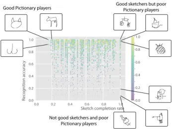
Revealing good and bad human Pictionary players.In Figure 2, we show average recognition accuracy of 1000 randomly selected
sketches from 20 categories from the QuickDraw dataset at different
sketch completion rates.The completion rateis the ratio of the length of drawn strokes (in pixels) to the total number of pixels in a sketch.
The cluster of sketches in the top right corresponds to complete
and detail-rich sketches that are well recognized: Those of good
sketchers, but weak Pictionary players. The sketches in the bottom
right correspond to complete and detailed but non-recognizable
sketches: those of bad sketchers. The top left of the plot is of
par-ticular interest, as it reflects sketches drawn by people potentially
Good Pictionary players Good sketchers but poorPictionary players
Not good sketchers and poor Pictionary players
Sketch completion rate
Rec og nition ac cur ac y 0.0 0.2 0.4 0.6 0.8 1.0 0.0 0.2 0.4 0.6 0.8 1.0 0.0 0.2 0.4 0.6 0.8 1.0
Fig. 2. Sketch recognizability versus sketch completion rate. Plot shows den-sity, encoded both with the color and size of the points. (Top left) Sketches of good Pictionary players, (top right) sketches of good sketchers but poor Pictionary players, and (bottom left and right) sketches of bad sketchers and poor Pictionary players.
0.0 0.2 0.4 0.6 0.8 1.0 0.0 0.2 0.4 0.6 0.8 1.0
Sketch completion rate Original human strokes order 0.0 0.2 0.4 0.6 0.8 1.0 0.0 0.2 0.4 0.6 0.8 1.0 Original human strokes order (b) Face (a) Average over several categories
Sketch completion rate
Cor
rec
t class sc
or
e
Fig. 3. Recognizability scores (Sketch-a-Net 2.0 [Yu et al. 2017]) at various levels of sketch completion for a randomly selected subset of sketches from the QuickDraw dataset [Ha and Eck 2018]. Dashed lines indicates the original human sketching strategy, shaded area indicates the region between the best and worst possible sketching strategies, obtained with a coarse exhaustive search.
good at a Pictionary game –they are able to produce recognizable sketches with very few strokes.
The gap between good and bad stroke order. Figure 3 shows that stroke order plays a crucial role in the early recognition of a sketch.
The dashed line indicates how the recognizability (using
Sketch-a-Net 2.0 [Yu et al. 2017]) of the partial sketches increase as more detail
is added – when following the original human sketching order. We
perform a coarse exhaustive search (described in detail in Section
4.1.1) over stroke order in each human sketch to find the best- and
worst-possible stroke sequences for early recognition, representing
by the top and bottom of the colored area. From the plots, it can
be seen that: (1) There is a significant gap between the upper- and
lower-bound, confirming that stroke order is indeed a dominating
factor for early sketch recognizability. (2) Human sketch order is
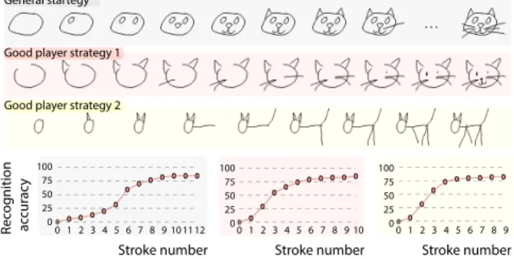
Good player strategy 2 General startegy
Good player strategy 1
100 75 25 0 50 100 75 25 0 50 100 75 25 0 50 0 1 2 3 4 5 6 7 8 9 0 1 2 3 4 5 6 7 8 9 10 0 1 2 3 4 5 6 7 8 9 10 11 12
Stroke number Stroke number Stroke number
Rec og nition ac cur ac y
Fig. 4. Example human strokes ordering strategies. Grey: General strategy. Red and Yellow: Two alternative sketching strategies of the good Pictionary players. The graphs show the prediction probability of each sequence at each accumulated stroke. It can be seen that sketches of good players are recognized earlier.
human participants in QuickDraw generally prioritized drawing
salient strokes first (Figure 3 a). (3) In most categories, there is still a
big gap between the human order and the optimal order (Figure 3 b).
This suggests that – even if using the same set of stroke primitives –
an AI agent has scope to compete with humans at Pixelary simply by
learning a better stroke-sequencing strategy. This is the motivation
behind the training setting of our AI drawing agent: it learns the
sequencing strategy by imitating the optimal stroke order rather
than the human one, which is sub-optimal for early recognizability
purposes.
The difference between strategies of bad and good human Pictionary players.We further compare ordering strategies of ordinary human Pictionary players with good players who achieve a recognizable
rendition early on. We make two key observations. First, there is
by-and-large a common ordering strategy among most humans, while
good sketchers often exploit diverse and distinct drawing strategies
(Figure 4). In Figure 5 we show kernel density plot of 128D Seq2Seq
autoencoder, trained separately on each category, features after PCA,
from two categories: cat and computer. It can be seen that there is
one dominating cluster of PCA features when we randomly sample
1K sketches from their respective categories. However, we see
multi-modal distributions emerging when we choose 1K samples from the
sketches of the good Pictionary players. The top 1K sketches are
chosen by considering the average recognition probability of the
accumulated strokes for each sketch.
Second, the optimal stroke orderings of strong human QuickDraw
players exhibit large jumps in-between consecutive strokes. The
average euclidean distance (in a 256×256 canvas) between the end-point and the start-point of consecutive strokes constitutes
94.62(±14.74)for the original strokes order and 115.16(±15.47)for the optimal stroke order. This is intuitive since humans tend to
complete one semantic part of the sketch before moving to the next
one (i.e., drawing all whiskers on one side of a cat face sketch before
moving to the other side. However, the complete part is often not
necessary for recognition, therefore the stroke sequencing strategy
that leads to early recognition may move away from this
part-by-part paradigm.
computer (random 1K sketches) cat (random 1K sketches)
computer (top 1K sketches)
PC1 PC1 PC1 PC1 PC 2 PC 2 PC 2 PC 2
cat (top 1K sketches)
Fig. 5. Kernel density plot of128D Seq2Seq autoencoder features projected
to principal component axes. (Left) Normal human data is uni-modal while top players (right) exhibit multi-modal strategies.
4 METHODOLOGY
Our goal is to obtain the sketching agent that produces recognizable
images with few strokes, as per top Pictionary players.
Unfortu-nately, only a small percentage of QuickDraw sketches satisfy this
criteria and are not sufficient for training. Therefore, as mentioned
earlier, there are two steps to training a strong Pixelary agent
(Fig-ure 6). (i) Our first step is generation of the optimal training set
from the (sub-optimal) QuickDraw human sketch dataset. (ii) The
optimally ordered QuickDraw dataset is used to train the generation
model. Steps (i) and (ii) could be performed jointly as a single step.
Nevertheless, since there is no information flow from (ii) to (i), it is
simpler to first pre-compute step (i).
4.1 Data reordering
In QuickDraw dataset, each category contains 75,000 sketches. Each
sketch has variable number of strokes. Exhaustively searching the
best stroke order in each sketch means evaluating each stroke
order-ing permutation. A sketch with 20 strokes would have 20!(2.43𝑒+18) permutations. Such process is computationally expensive and
in-feasible. QuickDraw contains approximately 220𝐾feasible sketches
with𝑁 <5 strokes and 500𝐾infeasible ones with𝑁 ≥8 strokes. We, instead, explore three alternative strategies: (1) coarse level
stroke reordering, (2) a greedy strategy of picking the next stroke
that maximizes the accuracy and (3) a neural sorting.
4.1.1 Coarse level stroke reordering.To obtain coarse stroke re-ordering, for each sketch we first iteratively group strokes into 5
stroke groups. At each iteration we identify the shortest stroke and
group it with the preceding or following neighboring stoke,
depend-ing which of them is shorter. We repeat this process till we obtain 5
stroke groups. 5 stroke groups give 5!(=120)possible stroke per-mutations. For each stroke groups permutation we computeEarly Recognition Efficacy (ERE)as the area under curve of correct recog-nition probability (using Sketch-a-Net 2.0 [Yu et al. 2017]) at each
stroke (ERE is formally defined in Section 6.1). We search for the
permutation of strokes groups with the highest ERE, and select this
Transformer Encoder Decoder MMD N(0,I) Latent vector: Z Data reordering Neural sorting Wasserstein Auto-Encoder
Optimal order sketch Reconstructed sketch
Fig. 6. A schematic illustration of the two step setting to train our stroke rendering agent –Pixelor. Yellow: Neural sort prediction for stroke-level order which
maximizes sketch recognition for the accumulated stroke representation. Red: Supervised training of Seq2Seq-WAE. We use Maximum Mean Discrepancy (MMD) [Gretton et al. 2012] as a divergence measure between two distributions.
4.1.2 Greedy approach.The greedy strategy is to sequentially pick a stroke that maximizes the immediate accuracy gain. The
compu-tation cost of such approach isO (𝑁2)classifier evaluations for𝑁 strokes.
4.1.3 Neural sorting.To obtain an optimal reordering we propose stochastic neural sorting [Grover et al. 2019] and optimize a
per-ceptual loss [ Johnson et al. 2016] in the form of recognizability as
assessed by Sketch-a-Net [Yu et al. 2017]. Each sketch is first passed
into an autoencoder to obtain its feature embedding. The sketch
embeddings scores, which are passed to a stochastic sorting
oper-ator, are obtained through a multilayer perceptron network those
parameters are optimized to obtain early recognition as judged by
Sketch-a-Net [Yu et al. 2017].
Sketch Embedding.The first step of our training model is obtain-ing the embedded representation of a sketch. We define a sketch
𝑋 =𝑠𝑗 𝑁 𝑗=1
as an ordered set of𝑁 strokes𝑠𝑗 andXas a set of all possible sketches. The setXalso contains partial/incomplete sketches which may not have a semantic meaning. We use an
en-coderF
𝜙∗ 1
:X →R𝐷, with parameters𝜙∗
1, as a feature extractor to
extract an embedding vector representing the sketch.F𝜙∗ 1
produces
a𝐷-dimensional embedding from a rasterized version of the sketch
𝑋 on a fixed sized canvas.F is realized using the Sketch-a-Net 2.0 [Yu et al. 2017] classifier up to a penultimate layer. Thus, the
sketch embedding is the 512𝐷output of the penultimate layer of
the Sketch-a-Net 2.0, where the parameters𝜙∗
1are trained through
Equation (4).
Scoring a Stroke. The embeddings of the full rasterized sketch𝑋 and its individual strokes rasterized on a fixed sized canvas together
serve as inputs to the neural sorting module. Stochastic neural
sorting, just like the classical sorting operator, operates on a set of
scalar values: thescoresof each element in a given set. The scores need to represent the relevance of each element for the downstream
task. In our case the elements are individual strokes and the task
is sketch recognition. As a scoring function𝑆𝜃 : R2𝐷 → Rwe use (a 3 layer multilayer perceptron neural network MLP) that
estimates the relevance score of each stroke of a sketch𝑋 with
respect to the full𝑋. The score vector of a sketch𝑋 is computed as r(𝑋;𝜃)=[𝑟1(𝑋;𝜃),· · ·, 𝑟𝑁(𝑋;𝜃)]
𝑇
, where𝑁is a total number of
strokes in the sketch𝑋, and
𝑟𝑗(𝑋;𝜃)=𝑆𝜃 h F𝜙∗ 1 𝑠𝑗 ;F𝜙∗ 1( 𝑋) i (1)
where{𝑠𝑗}is a singleton set of𝑗 𝑡 ℎ
stroke of𝑋 and[; ]represents the concatenation operator.F𝜙∗
1
𝑠𝑗 is the embedding of the
ras-terized individual stroke, andF𝜙∗ 1
(𝑋)is the embedding of the full rasterized sketch𝑋. Thus, the score𝑟𝑗(·)for stroke𝑗depends on the concatenated embedding of the𝑗th stroke and the full sketch.
Permuting Strokes.A sorting of𝑁elements is defined by an𝑁-D permutation. Following the notation of [Grover et al. 2019], we
denote a valid permutationz=[𝑧1, 𝑧2,· · ·, 𝑧𝑁] 𝑇
as a list of unique
indices from{1,2,· · ·, 𝑁}and the corresponding permutation ma-trix as𝑃z∈ {0,1}𝑁×𝑁whose entries are𝑃z[𝑖, 𝑗]=1𝑗=𝑧𝑖. The value of𝑧𝑖 denotes the index of the𝑖
𝑡 ℎ
most salient stroke of the given
sketch. With this definition, a sketch permuted by a given
permuta-tionzis expressed as𝑋z=𝑃z𝑋𝑇.
Sorting Strokes by Score. Let us now denote a potentially partial sketch 𝑋1→𝑛 ≜ 𝑠𝑗 𝑛 𝑖=1
as the set of its first𝑛strokes. By definition, a complete sketch is
𝑋1→𝑁. Towards fulfilling our end goal, we would like to have an optimally permuted sketch𝑋z∗ such that the incomplete sketch
(𝑋z∗)1→𝑛can be recognized for as low value of𝑛as possible. Hence, we formulate our learning objective for a single sketch𝑋as a
mini-mization of the negative log-likelihood of the correct label for every
sketch(𝑋z)1→𝑛: 𝐽(𝜃;𝑋)= 𝑁 Õ 𝑛=1 −logP h 𝑦=𝑌|F𝜙∗ 1 𝑃z·𝑋𝑇 1→𝑛 ;𝜙∗ 2 i with (2) 𝑃z=StochasticNeuralSort(r(𝑋;𝜃)), (3)
here𝑌is the true label of the sketch𝑋, StochasticNeuralSort(·) is the stochastic sorting operator [Grover et al. 2019] on the ordered
set of𝑁 scores andP[𝑦|·;𝜙∗
2] is a Sketch-a-Net [Yu et al. 2017]
classifier, through which we define a perceptual [Johnson et al. 2016]
rather than hand-crafted [Grover et al. 2019] loss. The minimization
is performed over the parameters𝜃of the scoring functionr(𝑋;𝜃), defined in Equation 1.
The early terms in the summation (i.e.,(𝑋z)1→1,(𝑋z)1→2,· · ·) will struggle to contribute this optimization, however, uniformly
optimizing over all of them encourages an ordering that maximizes
the chances of recognition as early on as possible.
Feature Extractor and Classifier.The parameterized feature ex-tractorF𝜙
1(·)
and classifierP[𝑦|·;𝜙2]are pre-trained jointly for the
sketch classification task as
𝜙∗ 1, 𝜙 ∗ 2 =arg min {𝜙1,𝜙2} Õ 𝑋∈Xb −logP𝑦|F𝜙 1(𝑋) ;𝜙2 , (4)
whereXbis the set of only complete sketches present in the dataset. For efficiency, the representations𝜙1and𝜙2are learned through
Eq 4, and fixed for subsequent training of the scoring model with
Equation (3). The vector𝜙1is the parameters of the Sketch-a-Net
2.0 [Yu et al. 2017] classifier up to a penultimate layer – the output
of this layer is a sketch embeddingF𝜙
1(·)
and𝜙2is the parameters
of the last layer that returns the classification scoreP[𝑦|·;𝜙2].
Optimal ordering.Optimizing𝐽(𝜃;𝑋)(Equation 2) with respect to𝜃, trains a stroke scoring function in such a way that when all
strokes are sorted by salience (Equation 3), the early recognition
according toPis maximized. The optimally sorted version of Quick-Draw for training a generation agent is obtained by permuting each
sketch𝑋 with the estimated sortingz∗as𝑃z∗𝑋𝑇. The re-ordering is independent per sketch, while learning𝜃aggregates performance
across all sketches.
Complexity.Our neural sorting method estimates a relevance score for each stroke in a given sketch inO (𝑁), and performs sort-ing inO (𝑁2)time for𝑁strokes. In the training phase, an additional
O (𝑁)classifier (loss) evaluations (Equation 2) are required. In prac-tice, the classifier (linear) cost dominates, thus learning to re-order
is fast. The complexity values of all considered methods are listed
in Table 5.
Implementation details.We implemented the scoring function𝑆𝜃
with an MLP of a structure 2×512→512→256→1, with each
hidden layer followed by a ReLU activation function and the final
score is activated with a Sigmoid(·) function. The only trainable parameters of the sorting module are the ones in this MLP (∼0.6𝑀). The Sketch-a-Net [Yu et al. 2017] is composed of a few sets of convolution-max pooling-ReLUblocks followed by an MLP. We set the temperature parameter of the stochastic neural search [Grover
et al. 2019]𝜏(𝑒)= 1
1+
√ 𝑒
at𝑒𝑡 ℎepoch, gradually reducing it towards
zero as the training progresses, forcing the sorting model to discover
the non-relaxed permutation matrix. For each sketch in the set of
70,000 training of each class, we infer the best stroke permutation.
4.2 Sequence-to-Sequence Wasserstein Auto-Encoder OurPixelorsketching agent is a sequence-to-sequence Wasserstein autoencoder, which is trained on the reordered data computed in the
previous section. We first describe our encoder/decoder architecture
and then provide a motivation for a Wasserstein autoencoder.
Sequence-to-Sequence. Pixeloris realized as a sequence-to-sequence encoder-decoder architecture. While the classic SketchRNN [Ha and
Eck 2018] uses bidirectional LSTM and autoregressive LSTM as the
encoder and decoder respectively, we replace the bidirectional LSTM
encoder by a Transformer [Vaswani et al. 2017] encoder to capture
better contextual information. Following SketchRNN [Ha and Eck
2018], we keep the autoregressive LSTM decoder with Gaussian
Mixture Model components.
Generative Sequence Models. In vanilla sequence-to-sequence mod-els such as SketchRNN, the encoder produces a mean vector and
(diagonal) covariance matrix with which a Gaussian distribution is
paramaterized. A random vector is then drawn from this Gaussian
which forms the input for the decoder. The difference between Pix-elorand prior VAE-based work, such as SketchRNN, lies in how the distribution of latent vectors is constrained. The distribution of
la-tent vectors is important because we need to generate adistribution of new sketch without any referencesuch as an input sketch or photo. In SketchRNN’svariationalautoencoder the distribution of latent vectors is controlled via the famous variational lower bound:
inf 𝐺(𝑋|𝑍) ∈ G inf 𝑄(𝑍|𝑋) ∈ Q E𝑃𝑋 KL(𝑄(𝑍|𝑋), 𝑃𝑍) −E𝑄(𝑍|𝑋)[log𝑝𝐺(𝑋|𝑍)] , (5)
where𝑃𝑋 is the real data distribution,𝑃𝑍is the prior distribution
over latent vectors (here it is a standard Gaussian),𝑄(𝑍|𝑋)is a prob-abilistic encoder, and𝐺(𝑋|𝑍)is a deterministic decoder. Both𝑄(·) and𝐺(·)are realized by neural networks, thus the infimum operator over sets (QandG) corresponds to the minimization over network parameters. This model struggles with matching multi-modal
distri-butions because of the form of reverse KL divergence, which results
in the requirement of training SketchRNN separately for each object
category [Chen et al. 2017a]. As mentioned in Section 3, we observe
a multi-model distribution of optimal strategies already within a
single category. To alleviate this limitation we propose to use instead
a Wasserstein autoencoder.
Wasserstein autoencoder (WAE). The wasserstein autoencoder (WAE) is formulated as,
inf 𝐺(𝑋|𝑍) ∈ G inf 𝑄(𝑍|𝑋) ∈ Q E𝑃𝑋 E𝑄(𝑍|𝑋) 𝑐 𝑋 , 𝐺(𝑋|𝑍) +𝜆D (𝑄𝑍, 𝑃𝑍) (6)
where𝑐(𝑎, 𝑏)is an arbitrary function that measures the difference between𝑎and𝑏,Dis an arbitrary divergence between two dis-tributions, and𝑄𝑍 =E𝑃
𝑋[
𝑄(𝑍|𝑋)]. The first term in Equation 6 corresponds to the second term in Equation 5 as they are both
reconstruction losses.
The key difference is then how to realize the regularization term:
E𝑃𝑋
KL𝑄(𝑍|𝑋), 𝑃𝑍 (VAE) v.s.D (𝑄𝑍, 𝑃𝑍)(WAE). The difference between these two mechanisms matters, as VAE asks every sample’s
distribution to match the prior (standard Gaussian), which results
in asmall intersected areaas the overlap of samples’ posterior distri-butions. This will eventually lead to the lack of diversity/modality.
Instead,D (𝑄𝑍, 𝑃𝑍)employs a deterministic decoder, and matches one single posterior distribution (per mini-batch) with the prior
(standard Gaussian). As a result, the Wasserstein autoencoder
cre-ates awider spacefor latent vectors, and eventually promotes diver-sity. The choice ofDis flexible as long as it is a valid distribution divergence, and we use Maximum Mean Discrepancy (MMD)
[Gret-ton et al. 2012] for the ease of implementation as alternative choices,
which is less stable. We use an inverse multi-quadratic kernel, as
is used in the paper that introduced the Wasserstein autoencoder
[Tolstikhin et al. 2018].
Implementation details. We use the same data format for sketch coordinates as used by the classic SketchRNN, and the output
di-mension of the Transformer encoder is 512 with 4 heads and 2
stacked layers. The dimension of the feed forward network within
the transformer is 2048, we use the same parameter free positional
encoding layer as used by [Vaswani et al. 2017]. The value of𝜆in
Equation 6 is 100. Unlike LSTM, since the input and output
dimen-sion of transformer encoder are same, we use a simple linear layer,
shared across the time steps, to convert 5 elements sketch
represen-tation to a 512 dimensional vector at each time step of the sketch
sample. Instead of using the final time step’s output to predict the
distribution parameters, we perform a maxpooling operation over
the time steps and use it to predict the distribution parameters.
5 TRAINING DATA
We train our model using QuickDraw [Ha and Eck 2018], the largest
free-hand sketch dataset. We choose 20 object categories namely
bicycle, binoculars, birthday cake, book, butterfly, calculator, cat,
chandelier, computer, cow, cruise ship, face, flower, guitar, mosquito,
piano, pineapple, sun, truck and windmill; using 70,000 sketches
per category for training. In order to maintain the high quality of
the generated sketches, we train one separate sorting and synthesis
model for each category but share a common classifier as a judge.
However, we observed that having one classifier with too many
classes makes the sorting model relatively unstable to train. In our
experiments, we used two separate 10 class classifiers to train our
sorting model. We divide all the data into training and test splits,
by keeping a quarter of all sketches as a test set.
6 EVALUATION ON QUICKDRAW
In this section, we evaluate neural sorting ordering algorithm against
alternative ordering strategies and sketch generation models in
terms of early sketch recognition and diversity of generated samples.
In this section, recognition accuracy is judged by the Sketch-a-Net
[Yu et al. 2017] recognizer AI throughout. Our code is implemented
in PyTorch [Paszke et al. 2019].
6.1 Metrics
As a quantitative measure of early recognition we defineEarly
Recognition Efficacy(ERE) as the area under curve of the correct class probabilityP[𝑦=𝑌|𝑋𝑡]at different completion rates𝑡 ∈ [0,1]of a sketch, where𝑋𝑡=0and𝑋𝑡=1denote empty and complete sketches,
respectively. We compute an empirical estimate of this quantity as
a weighted summation over𝑇 discrete intervals
𝐸𝑅𝐸≈ 𝑇 Õ 𝑝=0 P h 𝑦=𝑌|F𝜙∗ 1 𝑋𝑝·Δ𝑡;𝜙∗ 2 i Δ𝑡 , (7) whereΔ𝑡=1/𝑇.
We measure quality and diversity by Frechet Inception Distance
(FID) [Heusel et al. 2017]. It is computed by evaluating the distance
between the activations of the second last layer of the pre-trained
Table 1. ANOVA results for the impact of each of the ordering strategies on the measure of early recognition efficacy (ERE), defined in Section 6.1.
Compared ordering strategies p-value
Human order vs Coarse exhaustive search 5e-12
Coarse exhaustive search vs Greedy 1.2e-6
Greedy vs Neural Sort 5.5e-15
Sketch-a-Net 2.0 classifier for generated sketches and real sketches
from the training dataset:
𝑑2=∥𝜇1−𝜇2∥ 2
+Tr(𝐶1+𝐶2−2
p
𝐶1𝐶2), (8)
where𝜇1,𝐶1and𝜇2,𝐶2are the mean and covariance of the
activa-tions for generated and real sketches respectively.
For the evaluation of all generation models with both metrics, we
generate 10,000 sketches for each baseline.
6.2 Ordering Strategies
We first validate the ability of our neural sorting ordering algorithm
to find a good stroke ordering. The neural sorting model for
reorder-ing the original data is compared against: (1) Usreorder-ing the raw data
from QuickDraw, in original human provided order, (2) A coarse
exhaustive search (Section 4.1.1) (3) A greedy strategy of picking
the next stroke that maximizes the accuracy (Section 4.1.2).
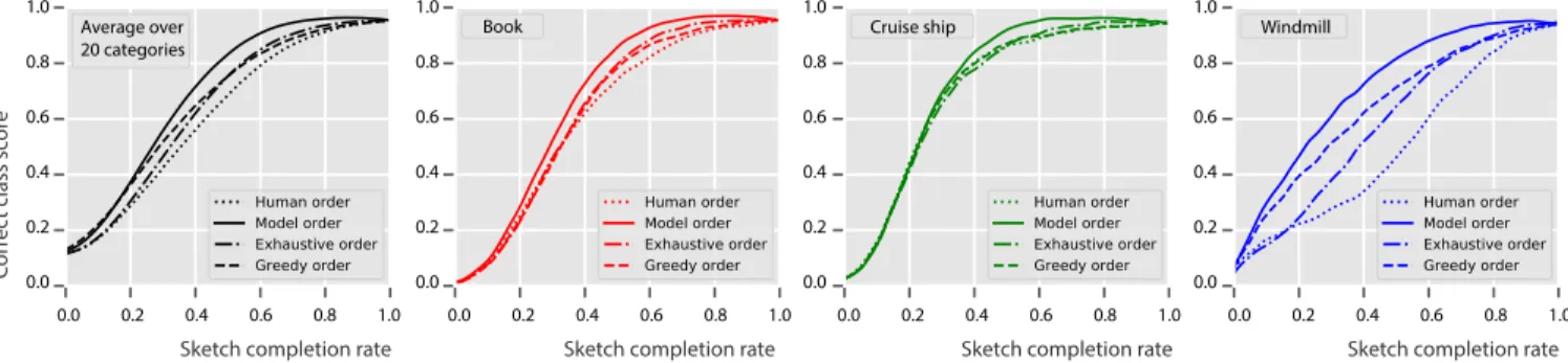
Neural Sort Improves Human Ordering in QuickDraw.Figure 7 shows the correct class probability (Sketch-a-Net AI judge) versus
pixel-level percentage of sketch completion. For neural sorting, we
evaluated all metrics on a held-out test-set comprising a quarter
of all sketches. All methods start with low recognition accuracy at
low sketch completion percentage and asymptote to high accuracy.
However better methods increase in accuracy quicker at a given
completion rate (closer to top-left corner). The average early
recog-nition efficacy (ERE) (Section 6.1) of sketches with original human
order of strokes is 0.612±.10. Greedy stroke search (dashed) im-proves on the original human order (dotted), with ERE of 0.665±.08. A coarse exhaustive search (dash-dotted) with 5 groups achieves
an ERE of 0.673±.08. Thus, both naive heuristics provide similar improvement on the original human data. Our neural sorter (solid)
achieves the best performance, reaching ERE of 0.715±.09, while still being quite efficient to evaluate. We analysed these results for
significance using ANOVA, which showed that each reordering
method improves statistically significantly in early recognition
com-pared to its predecessor in terms of the average ERE. The computed
p-values are shown in Table 1.
Neural Sort Convergence. Figure 8 analyses the convergence of our neural sorting method during training in terms of early
recog-nition efficacy of re-ordered human sketches (on a held-out
test-set comprising a quarter of all sketches) versus epochs on a few
representative categories. We can see that performance improves
continually as training proceeds, and surpasses the original
order-ing within 10 epochs of learnorder-ing. This confirms that neural sortorder-ing
works as expected, and crucially that it is possible to learn stroke and
0.0 0.2 0.4 0.6 0.8 1.0 0.0 0.2 0.4 0.6 0.8 1.0 0.0 0.2 0.4 0.6 0.8 1.0 0.0 0.2 0.4 0.6 0.8 1.0 0.0 0.2 0.4 0.6 0.8 1.0 0.0 0.2 0.4 0.6 0.8 1.0 0.0 0.2 0.4 0.6 0.8 1.0 0.0 0.2 0.4 0.6 0.8 1.0
Sketch completion rate
Cor
rec
t class sc
or
e
Sketch completion rate Sketch completion rate Sketch completion rate
Average over
20 categories Book Cruise ship Windmill
Fig. 7. Correct class probability for different orderings of QuickDraw strokes at different sketch completion rates. We compare correct class probability for the original human strokes ordering (dotted line), versus the following ordering strategies: coarse exhaustive search (dash-doted), greedy search (dashed line) and the proposed neural search (solid line). The curves are shown for the average of all 20 chosen categories and three distinct ones. The curves for all the categories individually are shown in the supplemental.
0.5 0.6 0.7 0.8 0.9 1.0 0.4 Ear ly R ec og nition Efficac y (ERE) Epochs 0 2 4 6 8 10 12 14 Chandellier Birthday cake Truck Binoculars Face Avg of 20
Fig. 8. Evolution of early recognition efficacy (ERE, Section 6.1) of re-ordered QuickDraw data over training epochs of or neural sort. For comparison, we show the ERE of original order as well (dashed lines).
(Equation 1) suitable for optimizing early recognition accuracy by
sorting.
Neural Sort Generalization.As described in Section 4, learning the parameters of the sorting model is reliant on a feature extractor and
a classifier already trained to be generalizable on new sketches. As
a result, the sorting model can be used on unseen sketches during
inference. We took advantage of it by training the sorting model on
a subset of the QuickDraw dataset and reordered all sketches only
by means of inference. Unlike with an exhaustive search or greedy
search, we are able to reduce the computational cost for the neural
sort by invoking the classifier while reordering the data. In our
experiments, we used 3/4 of the data for training, and reordered the entire dataset as a part of inference. We validate the ability of Neural
Sort to generalize by comparing the ERE scores across training set
sketches and unseen sketches – these are almost the same, 0.72±.07 and 0.71±.1, respectively.
6.3 Quality and Diversity of Generation
We first provide a detailed evaluation of an impact of the network
architecture choice on the diversity of the generated sketches and
0.0 0.2 0.4 0.6 0.8 1.0 Cor rec t class sc or e 0.0 0.2 0.4 0.6 0.8 1.0
Sketch completion rate Average over
20 categories
Fig. 9. Correct class probability for the sketches generated with our S2S-WAE, when trained on the data sorted with the neural sort (solid line), with greedy search (dashed line) or original QuickDraw data (dotted line). Correct class probability is an average over all 20 considered categories.
early sketch recognition, when trained on optimally sorted data. We
then compare the performance of our optimal suggested network
architecture versus SketchRNN [Ha and Eck 2018] on the original
and sorted data.
6.3.1 Impact of Model Components.As described in Section 4.2, the original SketchRNN uses Long Short-Term Memory (LSTM)
[Se-meniuta et al. 2016] both as an encoder and decoder and
Kullback-Leibler (KL) divergence as a distribution criteria. We evaluate the
performance when an encoder or/and decoder is a Transformer
net-work [Vaswani et al. 2017]. We as well, substitute variation lower
bound (Equation 5) with Wasserstein loss (Equation 6), and with
Maximum Mean Discrepancy (MMD) [Gretton et al. 2012]
distri-bution divergence measure. Table 2 shows that the optimal
per-formance in terms of both ERE and FID is obtained when we use
Transformer as encoder, in combination with MMD loss, which both
contribute to a better performance. We refer to this S2S-WAE model
asPixelor.
6.3.2 Pixelor performance.We compared the performance of both Pixelor, our S2S-WAE and the classic SketchRNN [Ha and Eck 2018]
Table 2. Ablation study of model components in terms of image generation quality measured by FID score mean and standard deviation. Training with neural-sorted data.
Model Encoder Decoder Prior FID Score ERE Sketch-RNN LSTM LSTM KL 10.17(1.94) 0.56 Variant-1 LSTM LSTM MMD 9.81(1.98) 0.59 Variant-2 Transformer LSTM KL 9.63(1.68) 0.63 Variant-3 Transformer Transformer KL 10.49(1.81) 0.61 Variant-4 Transformer Transformer MMD 10.32(2.01) 0.62 S2S-WAE (Ours) Tranformer LSTM MMD 9.06(1.86) 0.70
when trained with each dataset: the original QuickDraw stroke data,
and our neural sort optimized data.
Diversity.We evaluate the diversity of the generated samples in terms of FID scores ([Heusel et al. 2017] and Section (6.1)). Our
S2S-WAE has lower FID scores than the conventional Sketch-RNN, both,
when trained with the optimally ordered dataset or with the original
datatset (Table 3), an thus have higher quality of the generated data.
This is due to our ability to better handle the multi-modality of
optimally ordered data. The Sketch-RNN is unable to cope with
multi-modal distributions, and thus, when trained on the
optimally-ordered data, produces lower quality generations. Meanwhile, our
S2S-WAE is able to generate high quality images when training on
this optimally ordered dataset. FID score models the distribution as
a single Gaussian and compares it with the ground-truth
distribu-tion. Since in our case the optimally ordered dataset often can not
be modeled with a single normal distribution well, the FID scores
increase when trained on optimally ordered data. Please see the
supplemental for the break down of FID scores per category.
Early recognition. We evaluate early recognition through ERE (Eq. 7), by averaging the predicted probability value of the
ground-truth category of the sketches at 100 intervals. The results in
Ta-ble 3, show that: (1) our Seq2Seq-WAE architecture improves on
SketchRNN’s Seq2Seq-VAE in terms of early recognizability, no
mat-ter what data is used for training. (2) Training our model with
re-ordered data improves performance substantially. However, (3) only
our Seq2Seq-WAE is able to exploit the re-ordered data. SketchRNN’s
performance drops slightly when using the re-ordered data due to
its inability to exploit the multi-modality.
We further evaluate the quality of the fully generated sketches
by computing the classification accuracy with pre-trained
Sketch-a-Net 2.0. Overall our model generates more recognizable sketches
(Table 4), even when only late (rather than early) recognition is
considered. This is attributed to the better sequence to sequence
architecture of S2S-WAE compared to the classic SketchRNN.
The results in Figure 9 show the early recognition performance
of S2S-WAE generated sketches when trained with original human
data (dashed line), greedy ordering (dotted line), and our learned
neural sort ordering (solid line). We can see that our neural sort
ordering outperforms the competitors by a large margin.
6.4 Performance and complexity of reordering
Our optimal neural sort re-ordering strategy has comparable
run-time to the greedy strategy that picks a stroke to maximize the
Table 3. Early recognition efficacy (ERE) and image generation quality, evaluated through FID scores (lower is better), of generated sketches trained with original ordered data, and order estimated by NeuralSort. Accuracy is averaged across 20 classes. The values in braces indicate standard deviations.
Original order NeuralSort order
ERE FID ERE FID
S2S-WAE (Ours) 0.563 7.52 (1.72) 0.657 9.07 (1.86)
SketchRNN 0.532 8.95 (1.73) 0.526 10.18 (1.94)
Table 4. Classification accuracy of complete sketches generated by different synthesizers.
Orignal order NeuralSort order
S2S-WAE (Ours) 92.6% 94.9%
SketchRNN 89.0% 87.3%
Table 5. Computational complexity and practical single GPU run-time for reordering the2.4𝑀QuickDraw sketches of our chosen 20 classes. Classifier cost𝐶, scoring cost𝑆, strokes𝑁, stroke groups𝐺, backprop. epochs𝐸.
Complexity Approx runtime
Exhaustive search O (𝐶 𝑁!) est. 107days
Coarse Exhaustive search O (𝐶𝐺!) ∼60 days
Greedy O (𝐶 𝑁2) ∼8 days
Neural sorting (Ours) O ( (𝑆 𝑁2+𝐶 𝑁)𝐸) ∼15 days
accuracy gain. For our model, scoring is much faster than the
classi-fier (so𝑆≪𝐶) and the classifier evaluation (Sketch-a-Net inference
≈0.1𝑚𝑠on a standard GP U) dominates the cost. The alternatives have no scoring cost, but worse dependence on the classifier cost.
Our Neural Sort approach scales well, it is slower than Greedy
search, but provides improves early recognition of the ordered and
generated data. Furthermore, once trained it can be used to re-order
new data as onlyO (𝑆 𝑁2)cost (Section 6.2). 6.5 Discussion
Overall our results show that our Neural Sorting significantly
im-proves the ordering of QuickDraw data in a scalable manner.
Fur-thermore, our resultingPixeloragent can synthesize sketches that can be recognized more early than those in QuickDraw; and earlier
and more accurately overall than those generated by SketchRNN.
7 HUMAN STUDY
In this section, we perform a set of human studies to evaluate our Pixeloragent. In particular, we re-evaluate the previous comparisons on QuickDraw data, but using a team of human judges, rather than
Sketch-a-Net AI judge. More significantly, we collect a new dataset
of human sketches under favorable conditions designed for early
recognition termedSlowSketch, and comparePixelor’s performance against this new data under both AI and human judging.
7.1 Human Study Setup
Subset of QuickDraw sketches.We first evaluate how Pixelor, trained on optimally-ordered QuickDraw data, competes with the
human sketchers, who are limited by time constraints (all the
par-ticipants of QuickDraw datatset were limited by a 20-seconds time
frame) when evaluated by human judges. For this evaluation, we
randomly selected 12 sketches for each of 20 categories, listed in
Section 5 from both QuickDraw andPixelorgenerated data.
Sketching attempt number
1 2 3 4 5 6 7
0 0.2 0.4 0.6 0.8 1
Color encoding: normilized stroke number
Fig. 10. Visualization of the sketches of the ‘cat’ category by two partici-pants from theSlowSketchdatatset.
Newly collected human sketches - SlowSketch.We next built a custom interface to collect a new set of test data, where human
observers are not limited by any time constraint, and are provided
with on-the-fly feedback about the confidence of recognition of
their sketches. The participants were asked to make sketches of 20
given categories. To help train participants to optimize for early
recognition, the sketching interface consisted of a canvas as well
as a plot that shows the score given by the Sketch-a-Net AI judge
for the desired category. Participants made at least 7 attempts per
category (Figure 10). In this way participants had the chance to
refine their sketching strategy to achieve earlier recognition by the
AI judge over repeated trials. We collected≈1700 sketches from 12 participants. A screenshot of the interface is provided in the
supplemental.
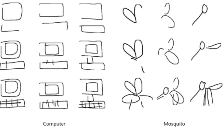
New QuickDraw New QuickDraw New QuickDraw
Bicycle Chandelier Cow
Fig. 11. Visual differences between newly collectedSlowSketchsketches
and samples from the QuickDraw dataset.
Analysis of SlowSketch. The newSlowSketchdata differs from the QuickDraw data in the amount of details and diversity of sketching
strategies as shown in Figure 11. We can see that the new sketches
are cleaner and more precise than QuickDraw, due to the lack of
(clock) time pressure. To study the affect of multiple practice trials,
the ERE (AI Judge) scores of the human sketches vs trials are plotted
in Figure 12. We can see that performance slowly improves with
sketching attempts, after some exploration of extreme strategies on
the second attempt.
Sketching attempt ERE 1 2 3 4 5 6 7 0.0 0.2 0.4 0.6 0.8 1.0 0.48 0.26 0.40 0.25 0.54 0.22 0.52 0.20 0.55 0.21 0.56 0.20 0.61 0.20
Fig. 12. Early Recognition Efficacy (ERE) of new human sketches in the new
SlowSketchdataset at the different attempt numbers. ERE improves slightly
with practice.
Human AI Competition: Data Preparation. To organize the data for a fair comparison of sketching efficiency, we need to normalize
for physical drawing speed and scale. We centered and scaled all
the sketches so that their area matches a canvas size 256×256 pixels. To control for drawing speed, we then establish pixel-level
synchronization. We compute the length of all sketches and select
the one with the largest value. We then pad all the sketches to have
the same length by repeating the last sub-stroke of a sketch. This
does not visually alter the appearance of the sketch, or the early
recognition time. But it does allow all sketches to be compared
evenly in terms of % of pixel completion.
For newly collected human sketches, for each participants and
each category we select one sketch out of 7 for subsequenthuman judgeevaluation, asthe sketch with the shortest total length. This corresponded to the 4th attempt on average, which is the middle
practice trial out of seven. We later show in terms of ERE scores
that the selected sketch are indeed representative of the whole set
(Figure 14). Note however that the shortest sketch is likely to have
the best early recognition properties for human observers among
all 7 attempts.
Metrics.We employ different metrics for when the judge is hu-man or AI. For AI judge, we measure the early recognizability of
sketches through the previously defined ERE (Section 6.1), which is
an approximation of a continuous measure. For human judge, we
resort to two discrete measures. First, we compute an average (the
ratio of the length of drawn strokes in pixels to the total number of
pixels in a sketch) for all correct guesses made by human within a
given category – smaller number indicates better early
recognizabil-ity. Second, we evaluate an average amount of the correct guesses –
larger number indicates better recognizability.
Pixelor Training. For the comparisons in this section, the same Pixeloras in Section 6 is used. That is, it is trained on re-ordered QuickDraw data.
7.2 AI judge
We first comparePixelorsketch generation with those drawn in our SlowSketchdataset, and those of QuickDraw, when judged for early recognition by the AI classifier Sketch-a-Net 2.0 [Yu et al. 2017].
166:12 • Ayan Kumar Bhunia, Ayan Das, Umar Riaz Muhammad, Yongxin Yang, Timothy M. Hospedales, Tao Xiang, Yulia Gryaditskaya, and Yi-Zhe Song
cat
cat butterfly
Fig. 13. Top row in each section shows the sketch generated byPixelor, while the second row shows human drawing inSlowSketch.
provides the best early recognition performance. On average, the
newlySlowSketchhuman sketches are correctly recognized at 33% of sketch completion whilePixelorones already at 17%. (The sketch is considered to be correctly recognized when the accuracy of the
true class is higher than 0.5.) Only 68% of complete human sketches
are correctly recognized, compared to 85% for the randomly selected
subset ofPixelorsketches, used in this study.
Surprisingly, the AI classifier performs much worse on the newly
collectedSlowSketchsketches than on the QuickDraw human sketches. This is due to the discrepancy between the style of QuickDraw
sketches on which the recognition AI was trained, and those in the
new dataset (Figure 11). Thus the humanSlowSketchsketches here are scored unrealistically badly, and this result should not be taken
very literally. We do also compare the performance on the selected
sketches (previous section) with the average performance and see
that the performance is similar. Thus the selected sketches can be
considered representative of human performance inSlowSketch. In the next section we repeat the evaluation with human judges,
which we assume provides gold-standard recognition such that the
dataset bias between QuickDraw andSlowSketchcan be ignored.
Cor
rec
t class sc
or
e
Sketch completion rate
0.0 0.2 0.4 0.6 0.8 1.0 0.0 0.2 0.4 0.6 0.8 1.0
Fig. 14. Comparison of early recognition performance forPixelor, human
Quickdraw and humanSlowSketchsketches (both selected and average).
The shown curves are computed by averaging the correct class probabilities of all sketches at each completion rate.
7.3 Human judging
In this section we evaluatePixelorvs QuickDraw humans andPixelor vsSlowSketchhumans under human judging in two independent studies with non-overlapping sets of participant judges.
Interface. We created an on-line interface, where the participant judges are shown one sketch at a time and do not know if it is a
human or AI sketch. Participants are able to explore a sketch
unfold-ing dynamically by movunfold-ing a slider (only the movement forward
is possible) in 5% completion intervals. Below the canvas with the
sketch, we showed 20 categories and asked the judge to guess as
soon as they think they recognize the shape. An screenshot of the
interface is shown in the supplemental.
Pixelor vs QuickDraw humans. In the first study, 8 participant judges provided 1920 guesses in total. In each trial they were
ran-domly shown either a sketch from QuickDraw dataset or aPixelor sketch. We recorded the completion step at which they first correctly
recognized the sketch.
In this setup, humans are able to recognize Pixelor sketches slightly faster than the sketches from the QuickDraw dataset. The
average correct guess for the QuickDraw sketches was done at 29.5%
of sketch completion, while forPixelorat 28.2%. We performed an ANOVA analysis which shows thatPixelorwins statistically signifi-cantly on average with𝑝-value of 5𝑒−4. Moreover, if we analyze each category individually and fix the significance threshold at 5𝑒−3, Pixelorwins statistically significantly on 6 categories and loses just on 2. The total number of correct guesses for thePixelorsketching sequences is also higher than for Quickdraw: 82% versus 79%. Thus,
in summary, we can see thatPixelorsystematically outperforms the humans of QuickDraw.
Pixelor vs SlowSketch humans. In the second study another 8 par-ticipant judges took part, and were prompted to guess on a mix of
Pixelorand newly collectedSlowSketchhuman sketches. We again collected 1920 guesses. For each category we compute the average
sketch completion rate when the correct guess was made. The
re-sults in Figure 15 show thatPixelorperforms comparably to human performance: The average correct guess for Humans is at 31% of the
sketch completion vs 33% for AI sketches. On average, significance
analysis shows thatPixelorloss is statistically significant with𝑝 -value of 4𝑒−4. However, when we fix the significance threshold for each category at 5𝑒−3, we see the performance is almost the same on Human andPixelorgenerated sketches:Pixelorwins on 4 and loses on 5. Please see the supplemental for category-wise𝑝-values.
On average human judges made a correct guess on 78.2% ofPixelor sketches and 79.0% of human sketches. This similar recognition rate
and win/loss ratio indicates that overallPixelorcan be considered to perform comparably to the favorably evaluatedSlowSketchhumans.