probabilistic prediction
Submitted by
Raisa Dzhamtyrova
for the degree of Doctor of Philosophy of the
Royal Holloway, University of London
I hereby declare that this thesis and the work presented in it is entirely my own. Where I have consulted the work of others, this is always clearly stated.
Raisa Dzhamtyrova
Supervisor and Examiners Supervisor: Dr Yuri Kalnishkan
Internal Examiner: Dr Vadim Shcherbakov
The goal of this thesis is to develop new competitive online algorithms for making predictions. In online learning, as in real life, signals arrive sequentially, and decisions should be adjusted in regard to new information. In the competitive prediction frame-work, predictions are made by experts and a learner. The goal of the learner is to make predictions which are not too much worse than the best expert. The quality of the prediction is measured by the cumulative loss.
Our starting point is the Aggregating Algorithm (AA) which optimally merges experts’ predictions and provides a theoretical guarantee on its performance in com-parison with the best expert. An important feature of the AA is that it works under any circumstances and it does not require any statistical assumptions. For a lot of loss functions, the strategy of the AA predicts as well as the best expert. In other cases, it is possible to apply the Weak Aggregating Algorithm (WAA), which provides a weaker theoretical guarantee but still resolves the problem of competitive prediction.
In this thesis, we provide algorithms with strong theoretical guarantees for many loss functions and different sets of experts. We start with the generalisation of the AA with finitely many experts for prediction of vector-valued outcomes. We propose a number of merging algorithms for prediction of vector-valued outcomes with tight worst-case loss upper bounds similar to those for the AA. Another approach of applying the framework of prediction with expert advice with finitely many models is proposed for estimation of Value at Risk.
It is possible to achieve good theoretical guarantees even if the set of experts is infinite. In the second part of the dissertation, we provide competitive algorithms for making probabilistic predictions. The first proposed algorithm, which combines the class of quantile regression experts, can be used for making interval predictions. The second approach merges the class of linear regressions and output forecasts in the form of the cumulative distribution functions.
In this dissertation, an important problem of probabilistic multi-class classification is considered. The approach which combines the class of multinomial logistic regressions is proposed to solve this problem. The strategy is competitive in terms of the Kullback-Leibler cumulative loss.
The theoretical guarantees of the proposed algorithms are proven and experiments on artificial datasets and real-world datasets are conducted. Empirical results empha-sise the properties of new algorithms and demonstrate that they have a good perfor-mance in practice.
I am grateful to my supervisor Yuri Kalnishkan for introducing me to the area of prediction with expert advice and providing help and guidance during my PhD. This research showed me new ways to approach and solve scientific problems. It has been an invaluable and exciting experience.
I thank my grandmother, parents and sister for their love and constant belief in me. Also I thank Marco Gorelli for his support and encouragement, it helped me a lot to stay positive and continue my work.
This research was made possible by the Reid Scholarship I was awarded from the Computer Science Department at Royal Holloway, for which I am very grateful. I thank all the staff of the Computer Science Department for providing a very friendly research environment and their help. I am grateful to the college for funding my trips abroad to present papers at conferences.
1 Introduction 9
1.1 Original contributions . . . 11
1.2 Publications . . . 11
1.3 Structure of the thesis . . . 12
2 Main algorithms 13 2.1 Framework . . . 13
2.2 Aggregating Algorithm. . . 14
2.2.1 Description of Aggregating Algorithm . . . 14
2.2.2 Some examples of mixable games . . . 18
2.3 Aggregating Algorithm for Regression . . . 22
2.4 Aggregating Algorithm with Discounting. . . 24
2.5 Weak Aggregating Algorithm . . . 28
3 Aggregating Algorithm for prediction of packs 30 3.1 Introduction. . . 30
3.2 Preliminaries and Background. . . 33
3.2.1 Protocols for Prediction of Packs . . . 33
3.2.2 Delayed Feedback Approach . . . 34
3.3 Mixability . . . 36
3.4 Algorithms for Prediction of Packs . . . 39
3.4.1 Prediction with Plain Bounds . . . 39
3.4.2 Prediction with Bounds on Pack Averages . . . 41
3.5 Discussion and Optimality . . . 43
3.5.1 A Mix Loss Lower Bound . . . 44
3.6 Experiments. . . 45
3.6.1 Datasets and Experts . . . 46
3.6.4 Improving Predictions with Inflation Data . . . 58
3.6.5 Conclusions . . . 60
4 Weak Aggregating Algorithm for Value at Risk 63 4.1 Introduction. . . 63
4.2 Framework . . . 65
4.3 Experiments. . . 66
4.3.1 WAA for normal distributions. . . 66
4.3.2 WAA for conventional models . . . 67
4.3.3 Backtesting . . . 73
4.4 Conclusions . . . 78
5 Universal algorithms for quantile regression 80 5.1 Introduction. . . 80
5.2 Framework . . . 82
5.3 Theoretical Bounds for WAAQR . . . 83
5.4 Prediction Strategy. . . 86
5.5 Experiments. . . 87
5.5.1 WAA . . . 88
5.5.2 WAAQR . . . 89
5.6 Conclusions . . . 93
6 Competitive online regression under Continuous Ranked Probability Score 99 6.1 Introduction. . . 99
6.2 Framework . . . 100
6.3 Theoretical Bounds . . . 102
6.4 Prediction Strategy. . . 102
6.5 Proof of Theoretical Bounds . . . 107
6.6 Experiments. . . 108
6.6.1 Synthetic Dataset . . . 108
6.6.2 Solar Power Dataset . . . 110
6.7 Conclusions . . . 111
7 Universal algorithms for probabilistic multi-class classification 115 7.1 Introduction. . . 115
7.4 Prediction Strategy. . . 120
7.5 Proof of Theoretical Bounds . . . 123
7.6 Kernelized Algorithm . . . 127
7.7 Experiments. . . 132
7.7.1 Synthetic Dataset . . . 132
7.7.2 Glass Identification Dataset . . . 133
7.7.3 Football Dataset . . . 135
7.7.4 Conclusions . . . 137
8 Conclusions 139
Bibliography 140
R the space of real numbers
Rn then-dimentional space of real numbers
X0 transpose of matrixX
kxk1 L1-norm of x∈Rn
kxk2 the Eucledian norm (L2-norm) ofx∈Rn
kxk∞ the maximum norm of x∈Rn
S strategy of the learner
Sθ strategy of the expertθ
LT loss of the learner at timeT
AA Aggregating Algorithm
AAD Aggregating Algorithm with Discounting AAP Aggregating Algorithm for Prediction of Packs AAR Aggregating Algorithm for Regression
APA Aggregating Pseudo-Algorithm
CRPS Continuous Ranked Probability Score EWMA Exponential Weighted Moving Average
GARCH Generalised Autoregressive Conditional Heteroskedasticity GBDT Gradient Boosting Decision Trees
MCMC Markov Chain Monte Carlo
MLR Multinomial Logistic Regression
QR Quantile Regression
QRF Quantile Random Forests
RF Random Forests
RKHS Reproducing Kernel Hilbert Space
VaR Value at Risk
WAA Weak Aggregating Algorithm
Introduction
An expert is a man who has made all the mistakes which can be made, in a narrow field
Niels Bohr
In everyday life people make their decisions based on predictions. For example, we make plans for a weekend based on a weather forecast or buy stocks of some company based on financial experts’ predictions of their prices. Usually predictions are made by an algorithm which learns from past experience. The goal of this thesis is to develop online competitive algorithms for making predictions with theoretical bounds on their performance. These bounds should hold for any future time point and without any stochastic assumptions.
In the real world we usually receive new information sequentially. Hence, we study the online setting in which predictions and outcomes are given step-by-step. Contrary to batch mode, where the algorithm is trained on a training set and gives predictions on a test set, we learn as soon as new observations become available. For example, suppose that our aim is to predict outcomes of football matches of a new season based on data available from a previous season. A batch algorithm builds a model on previous season’s data and this model is used to make predictions for all matches of the current season. In the online setting we add data sequentially and adjust parameters of the model after each match. More formally, we consider an online protocol where at each trial a learner observes a signal given by nature and attempts to predict an outcome, which is shown to the learner later. The leaner’s performance is measured by means of the cumulative loss.
In this thesis, we consider the framework of online prediction with expert advice. At each trial we have access to predictions of experts and need to make a prediction
based on their past performance. In statistical learning, usually some assumptions are made about the mechanism that generates the data, and guarantees are given for the method working under these assumptions. For example, one may assume a linear dependence between electricity consumption and temperature and try to fit the best parameters for linear regression. Instead, we work in the adversarial setting where no assumptions are made about the data generating process.
In this thesis, we consider an approach called competitive prediction, where one provides guarantees compared to other predictive models that are called experts. Ex-perts could be human exEx-perts, complex machine learning algorithms or even classes of functions. We treat an expert as a black box, i.e., we are not interested in its internal work. Our goal is to develop a merging strategy that will perform not much worse than the best expert. As a result, we do not try to build a model that works under certain assumptions but try to combine predictions that are given to us by experts. One may wonder why we do not just use predictions of only one best expert from the beginning and ignore predictions of others. First, sometimes we cannot have enough data to identify the best expert from the start. Second, good performance in the past does not necessary lead to good performance in the future.
The learner in the game of prediction plays against nature and experts from some pool. The aim of the learner is to keep its total loss small compared to the total losses of any expert. One of the approaches which provides a theoretical guarantee on the learner’s performance is the Aggregating Algorithm (AA), which was first introduced inVovk (1990). AA works as follows: we assign initial weights to experts and at each step the weights of experts are updated according to their current performance. The approach is similar to the Bayesian method, where the prediction is the average over all models based on the likelihood of the available data and model’s prior distribution. For the case of finitely many experts, AA gives a guarantee ensuring that the learner’s loss is as small as the best expert’s loss plus a constant.
Even if the decision pool is infinite it is possible to achieve good theoretical guaran-tees. The history of algorithms competitive with large parametric classes of strategies can be traced back to universal portfolios by Cover and Ordentlich(1996) (a survey is provided byCesa-Bianchi and Lugosi(2006)), which apply in the context of investment decisions and compete against portfolio selection techniques. In that framework one is interested in maximising wealth, but the problem can be restated in terms of losses.
One can consider outcomes and predictions from the one-dimensional interval [0,1] and signalsxt∈Rn. A natural choice of competitor strategies are then linear functions
on xt. Vovk (2001) and Azoury and Warmuth (2001) propose an algorithm for this framework (Vovk-Azoury-Warmuth predictor, also known as the Aggregating
Algo-rithm for Regression) targeted at square loss. The resulting algoAlgo-rithm asymptotically performs as good as any linear regression in terms of the cumulative square loss up to a logarithmic term in the number of steps. Gammerman et al.(2004) obtain a kernelized version of the predictor. Zhdanov and Kalnishkan (2013) study similar competitive bounds for standard ridge regression. In this thesis, we primarily consider the prob-lem of combining different classes of experts. These algorithms are called universal
algorithms because they are competitive with any expert from the chosen class.
1.1
Original contributions
1. The generalisation of the Aggregating Algorithm is developed for prediction of vector-valued outcomes called packs. Three algorithms for this new setting are proposed (Algorithm 6, Algorithm 7 and Algorithm 8) and guarantees on their performances are proven (Theorem 3.4.1 and Theorem 3.4.2). Experimental re-sults on sport and house price datasets are performed to compare algorithms. 2. A new approach to applying the method of prediction with expert advice is
pro-posed for calculating Value at Risk. Experiments and comparisons with existing methods are performed with stocks of three companies.
3. Universal algorithms for probabilistic predictions are developed and performance guarantees are proven for the following settings: quantile regression under pin-ball loss function (Section 5.4 and Theorem 5.3.1) and linear regression under Continuous Ranked Probability Score (Section6.4and Theorem6.3.1). Practical experiments show the performance of algorithms for renewable energy forecasting. 4. Universal algorithm for probabilistic multi-class classification under Kullback-Leibler game (Section 7.4 and Theorem 7.3.1) and its generalisation for Hilbert spaces (Section 7.6 and Theorem 7.6.4) are developed and their performance guarantees are proven for the class of multinomial logistic regressions.
1.2
Publications
The results described in this thesis are published either as conference proceedings or journal papers. The paper ‘Competitive Online Regression under Continuous Ranked Probability Score’ received the best student paper award.
1. Raisa Dzhamtyrova and Yuri Kalnishkan. Competitive Online Generalised Linear Regression with Multidimensional Outputs. In Proceedings of the International
2. Raisa Dzhamtyrova and Yuri Kalnishkan. Competitive Online Regression un-der Continuous Ranked Probability Score. In Proceedings of Machine Learning Research, the 8th Symposium on Conformal and Probabilistic Prediction with
Ap-plications, 2019, pages 105: 178–195
3. Raisa Dzhamtyrova and Yuri Kalnishkan. Universal algorithms for multinomial logistic regression under Kullback-Leibler game. Neurocomputing, 2019.
4. Dmitry Adamskiy, Tony Bellotti, Raisa Dzhamtyrova, and Yuri Kalnishkan. Ag-gregating algorithm for prediction of packs. Machine Learning, 2019, pages 108: 1231–1260.
1.3
Structure of the thesis
Chapter2 gives an overview of prediction with expert advice and the main algorithms which are used to derive the new proposed algorithms. Chapter 3 is devoted to the problem of generalisation of the Aggregating Algorithms for prediction of packs. Chap-ter 4describes a new approach to applying prediction with expert advice to calculate Value at Risk. In Chapter5 the new universal algorithm for quantile regression under pinball loss is developed. Chapter6describes the competitive strategy for online linear regression under Continuous Ranked Probability Score. Chapter 7 gives new ways of approaching the problem of probabilistic multi-class classification.
Main algorithms
In this chapter, we describe the main algorithms that are used in this work. This is the only chapter in the thesis where materials are not original, except for the proof of Lemma2.4.2.
2.1
Framework
In the framework of prediction with expert advice we need to specify agame G which contains three components: a space of outcomes Ω, a decision space Γ, and a loss functionλ : Ω×Γ → R. Thelearner or prediction strategy in the game of prediction plays against experts θ from some pool Θ and nature. At each step t experts output their predictions ξt(θ) ∈ Γ. After seeing all experts’ predictions, the learner outputs prediction γt ∈ Γ. After nature announces an outcome yt ∈ Ω, the experts and the learner suffer losses λ(yt, ξt(θ)) and λ(yt, γt) respectively. The aim of the learner is to keep its total loss Lt small compared to the total losses Lθt of all experts θ ∈ Θ. Sometimes we refer to the prediction strategy of the learner as S and the prediction strategy of the expert θ as Sθ. We define regret to be the difference between the cumulative losses of the best expert and the learnerRt=Lt−minθ∈ΘLθt.
Experts could be human experts, complex machine learning algorithms or even classes of functions. In Chapters3 and 4, we consider a finite number of experts and treat an expert as a black box, i.e., we are not interested in its internal work. In the rest of the thesis we consider parametrised classes of experts, such as the class of quantile regressions (Chapter 5), the class of linear regressions (Chapter 6) and the class of multinomial logistic regressions (Chapter7).
Below is the protocol of competitive online prediction: Protocol 1.
L0 := 0 Lθ0 := 0 for t= 1,2, . . . Experts output ξt(θ)∈Γ, θ∈Θ Learner outputs γt∈Γ Nature announces yt∈Ω Lt:=Lt−1+λ(yt, γt) Lθt :=Lθt−1+λ(yt, ξt(θ)), θ∈Θ end for
2.2
Aggregating Algorithm
2.2.1 Description of Aggregating Algorithm
One of the algorithms that can be used to solve the problem of prediction with expert advice is the Aggregating Algorithm (AA). We formulate the Aggregating Algorithm followingVovk(1990,1998,2001). The algorithm is based on the notion ofmixability. Consider a game G=hΩ,Γ, λi. A constantC > 0 isadmissible for a learning rate
η > 0 if for every θ ∈ Θ, every set of predictions ξ(θ) ∈ Γ, and every distribution P(dθ) (such that R
θ∈ΘP(dθ) = 1) there is γ ∈ Γ ensuring for all outcomesy ∈ Ω the inequality λ(y, γ)≤ −C η ln Z θ∈Θ e−ηλ(y,ξ(θ))P(dθ) . (2.1)
The mixability constant Cη is the infimum of all C > 0 admissible for η. This
infimum is usually achieved. For example, it is achieved for all η > 0 whenever Γ is compact ande−λ(γ,y) is continuous inγ.
An example of games G=hΩ,Γ, λi includesimple prediction game:
Ω = Γ ={0,1}, λ(y, γ) = 0, ify=γ, 1, otherwise .
Therefore, the learner tries to predict a binary sequence, 0 or 1; it suffers loss 1 if it makes a mistake. The logarithmic loss game:
Ω ={0,1}, Γ = [0,1], λ(y, γ) = −lnγ ify= 1, −ln(1−γ) ify= 0,
and thesquare-loss game:
Ω = [A, B], |A|,|B|<∞, Γ =R, λ(y, γ) = (y−γ)2
will be described in Section2.2.2. More examples of games can be found in Section 2 ofVovk (2001).
The Aggregating Algorithm takes a learning rate η > 0, a constant C admissible forG withη, and a prior distribution on experts P0(dθ). After each step t it updates the experts’ weights according to their losses:
Pt(dθ) =e−ηλ(yt,ξt(θ))Pt−1(dθ). (2.2) The weights of experts which suffer large loss at some step will have a smaller impor-tance for making further predictions. The prior distribution P0(dθ), which specifies the initial weights of experts, is an arbitrary distribution. Thus, any distribution can appear asPt−1(dθ), and inequality (2.1) holds for any P(dθ).
First, we introduce the Aggregating Pseudo-Algorithm (APA). A generalised
pre-diction is defined to be any function of the type Ω → [0,∞]. The APA suffers loss
gt(yt) after choosing generalised predictiongtat timetwhen the actual outcome isyt. The APA outputs at timetthe generalised prediction which is the weighted average of experts’ predictions: gt(y) =− 1 η ln Z Θ e−ηλ(y,ξt(θ))P∗ t−1(dθ), (2.3)
wherePt∗−1(dθ) are normalized weights:
Pt∗−1(dθ) =
Pt−1(dθ) Pt−1(Θ) ,
where Θ is a parameter space, i.e. experts θ ∈ Θ can output prediction ξt(θ) ∈ Γ at timet.
The AA is obtained from the APA by replacing each generalised predictiongt bya
permitted prediction Σ(gt), where the substitution function Σ maps every generalised
predictiong into a permitted prediction Σ(g)∈Γ satisfying
∀y:λ(y,Σ(g))≤Cg(y). (2.4) By putting (2.3) in (2.4), we get (2.1). We also need to define asuperprediction, which is a generalised prediction minorised by the loss of some prediction, i.e., a superprediction
is a function f : Ω→ [0,+∞] such that for some γ ∈Γ we havef(y) ≥λ(y, γ) for all y∈Ω.
We will assume that the substitution function, which attains inequality (2.4), exists. The AA requires that a ‘minimax’ substitution function should be chosen (Vovk(1990))
Σ(g)∈arg min γ∈Γsupy∈Ω
λ(y, γ)
g(y) . (2.5)
However, in some cases it is more computationally efficient to require that the substitution function follows
Σ(g)∈arg min
γ∈Γsupy∈Ω(λ(y, γ)−Cηg(y)) (2.6) and
(g1(y)−g2(y) does not depend ony)→(Σ(g1) = Σ(g2)), (2.7) where g1, g2 are the generalised predictions calculated with different weights distribu-tions. Assumption (2.7) is always compatible with (2.6) but is typically incompatible with (2.5). A great advantage of (2.7) is that we do not need to normalise experts’ weights at each step, and can calculate the pseudo-prediction from the unnormalised weights, since it will differ from (2.3) only by an additive constant.
The pseudo-code for the Aggregating Algorithm is given below. The Aggregating Algorithm
Initialize prior distribution on expertsP0(dθ) =P0∗(dθ),θ∈Θ, a learning rateη >0, an admissible constantC
fort= 1,2, . . . do
Get experts’ predictions ξt(θ),θ∈Θ. Calculate generalised prediction g: Ω→R,
defined bygt(y) =−1ηln
R Θe
−ηλ(y,ξt(θ))P∗
t−1(dθ), for ally∈Ω. Output predictionγt:= Σ(gt)∈Γ using a substitution function
Σ :RΩ→Γ, such that ∀y:λ(y,Σ(gt))≤Cgt(y). Read the outcome yt∈Ω.
Update the weights Pt(dθ) =e−ηλ(yt,ξt(θ))Pt−1(dθ),θ∈Θ. Normalize the weightsPt∗(dθ) = Pt(dθ)
R
θ∈ΘPt(dθ).
end for
andT = 1,2, . . . , the cumulative lossLT of the APA with parameters η and P0 follows LT(APA(η, P0)) =− 1 ηln Z θ∈Θ e−ηLθTP0(dθ). (2.8)
Proof. The lemma is proven by induction. It is obvious from (2.3) that (2.8) holds for
T = 1. Notice, that gT(yT) =− 1 ηln R Θe −ηλ(yT,ξT(θ))P T−1(dθ) PT−1(Θ) =−1 ηln R Θe −ηλ(yT,ξT(θ))e−ηLθT−1P0(dθ) R Θe −ηLθ T−1P0(dθ) .
Assume that (2.8) holds for T−1. Then
LT(APA) =LT−1(APA) +gT(yT) =−1 ηln Z Θ e−ηLθT−1P 0(dθ)− 1 η ln R Θe −ηLθ TP0(dθ) R Θe −ηLθ T−1P0(dθ) =−1 η ln Z Θ e−ηLθTP0(dθ).
The following lemma, which follows from Lemma 2.2.1 and (2.4), gives an upper bound on the cumulative loss of the Aggregating Algorithm.
Lemma 2.2.2. For a gameGwith an admissible constantC, a learning rateη, and any
priorP0, the following upper bound on the cumulative loss of the Aggregating Algorithm
holds for T = 1,2, . . . , LT(AA)≤ − C η ln Z θ∈Θ e−ηLθTP0(dθ). (2.9)
In case when the number of experts is finite we replace expert’s index θwith index i ∈ Θ = {1,2, . . . , N}. For the AA with a finite number of experts N we get the following lemma.
Lemma 2.2.3. For a game G with an admissible constant C, a learning rate η, and
the initial distribution on expertsp(i) (such that PN
i=1 = 1), the following upper bound
on the cumulative loss of the Aggregating Algorithm holds for T = 1,2, . . . ,
LT(AA)≤ − C η ln N X i=1 p(i)e−ηLiT ! ≤ −C η ln p(i)e−ηLiT =CLiT +C η ln 1 p(i). (2.10) An important class of the games aremixablegames withCachieving 1. The natural choice ofη is then the maximum value such that the mixability constantCη = 1, which
is the infimum of allC admissible forη; it minimises the second term on the right-hand side of (2.10). In particular, for mixable games with finite number of experts N and the uniform initial distribution on experts, the loss of the AA satisfies
LT(AA)≤LiT + 1
ηlnN, (2.11)
for i= 1, . . . , N. For non-mixable games (such as the absolute loss game withλ(y, γ) =
|γ−y|), bound (2.9) provides a trade-off. Optimising the bound is a more difficult task and may require assumptions on the behaviour of experts or the time horizonT.
2.2.2 Some examples of mixable games
In this section, we describe two important mixable games: the logarithmic loss game and the square-loss game. We show how to apply the AA for these games.
The logarithmic loss game
In this section, we discuss the logarithmic loss game G, where the outcome space Ω ={0,1}, the prediction space Γ = [0,1], and the loss function is defined as
λ(y, γ) = −lnγ ify= 1, −ln(1−γ) ify= 0, (2.12)
wherey∈Ω,γ ∈Γ. We will show that the Aggregating Algorithm for the logarithmic loss function withη= 1 is the same as the Bayesian mixture.
The weight updates (2.2) becomes
Pt(dθ) =ξt(θ)Pt−1(dθ) =P0(dθ)
t
Y
i=1
ξi(θ). (2.13)
Therefore, the normalized weights: Pt∗(dθ) = Pt(dθ)
R
ΘPt(dθ)
are identical to the posterior distribution of θafter observingy1, y2, . . . , yt.
The generalised prediction (2.3) becomes the loss of the Bayesian mixture gt(y) =−
1 ηln
Z
ξty(θ)Pt∗−1(dθ), (2.14)
whereξty(θ) is the prediction of the expert θfor the outcome y at the timet.
simplye−(.).The function xη is concave for η <1, and thus Z Θ (ξty(θ))ηQ(θ)≤ Z Θ ξty(θ)Q(θ) η
for any y and Q∈P(Θ).
After taking negative logarithms of both parts and multiplying by 1η, we obtain
−1 η ln Z Θ ξyt(θ)Q(θ) η ≤ −1 ηln Z Θ (ξty(θ))ηQ(θ).
In other words, the loss of the prediction corresponding to η = 1 is less than the generalised prediction calculated with any otherη <1.
The pseudo-code for the Bayesian Algorithm is shown below. The Bayesian Algorithm
Initialize prior distribution on expertsP0(dθ) =P0∗(dθ),θ∈Θ, fort= 1,2, . . . do
Get experts’ predictions ξt(θ),θ∈Θ. Output predictionγt=
R
θ∈Θξt(θ)P ∗
t−1(dθ). Read the outcome yt∈Ω.
Update the weights Pt(dθ) =ξt(θ)Pt−1(dθ),θ∈Θ. Normalize the weightsPt∗(dθ) = Pt(dθ)
R
θ∈ΘPt(dθ).
end for
The square-loss game
In this section, we consider the square-loss game, where the outcome space Ω = [A, B],
|A|,|B| < ∞, the prediction space Γ = R and the loss function λ(y, γ) = (y −γ)2.
The following lemma proves the mixability of the square-loss game with the restricted outcome space. The mixability for the outcome space Ω = [−Y, Y] is first proven in
Vovk (2001), the case of the outcome space Ω = [A, B] with an arbitrary interval is first described inZhdanov(2011).
Lemma 2.2.4. (Lemma 2.5 from Zhdanov (2011)). The square-loss game is
η-mixable if and only if η≤ 2
(B−A)2.
Proof. Consider the parametric curve {(λ(A, γ), λ(B, γ))|γ ∈ Γ}. Each point on this
curve corresponds to a prediction γ and the point’s coordinates are the losses when y =A or y= B occur. Let Λ ={(x, y)|there isγ ∈Γ :x ≥λ(A, γ) andy ≥λ(B, γ)}
The game is η-mixable if Cη = 1 for some η > 0, i.e., according to (2.4), we can find γ∈Γ such that
λ(A, γ)≤gt(A) λ(B, γ)≤gt(B) . (2.15)
The system has a solution if (gt(A), gt(B)) falls into the set of superpredictions. We apply the transformation Bη : [0,+∞]2 →[0,1]2 given by
x y ! → e −ηx e−ηy ! .
Under the transformationBη for the finite number of experts N, we need to solve the system: e−ηλ(A,γ) ≥e−ηgt(A)=PN i=1pt−1(i)e −ηλ(A,ξt(i)) e−ηλ(B,γ)≥e−ηgt(B)=PN i=1pt−1(i)e−ηλ(B,ξt(i)) .
The game is mixable if the system is solvable for all experts’ predictions and all nor-malised weights. This means that the convex combination should always fall in the set
Bη(Λ), which is possible if and only if the setBη(Λ) is convex. It is equivalent to find the values ofη for which the second derivative of the parametric curve
{(u, v) = (e−η(γ−A)2, e−η(γ−B)2)|γ ∈Γ} (2.16) is less or equal to zero.
The first derivative of the curve (2.16) is dv du = dv/dγ du/dγ = 2η(B−γ)e−η(γ−B)2 2η(A−γ)e−η(γ−A)2 = γ−B γ−Ae 2ηγ(B−A)−η(B2−A2).
And the second derivative of the curve is d2v du2 = d2v dudγ du dγ = B−A (γ−A)2 + 2η(B−A) γ−B γ−A e2ηγ(B−A)−η(B2−A2) 2η(A−γ)e−η(γ−A)2 ≤0. This is equivalent to (γB−−AA)2 1 2η(A−γ)+ (B−γ) ≤0. Thus, we have η ≤ 1 2(γ−A)(B−γ),
where γ ∈R. Since maxγ∈R(γ−A)(B−γ) = 14(B−A)2, the curve is concave if and only if η≤ 2
0
1
2
3
4
0
1
2
3
4
Figure 2.1: The parametric loss curve ((−1−γ)2,(1−γ)2), γ ∈[−1,1].
The Figure 2.1 illustrates an example of the parametric loss curve for the re-stricted square-loss game with the outcome space Ω = {−1,1}. Under the trans-formationBη, the set of permitted predictions is represented by the parametric curve
e−η(−1−γ)2, e−η(1−γ)2
, γ ∈[−1,1], which is shown in Figure2.2. The curve is convex forη≤ 1
2. The grey area in the Figure 2.2represents the set of superpredictions. Now we find a substitution function for the square-loss game with the outcome space Ω = [A, B]. Since we require the substitution function to follow (2.6), we have
(γ−B)2−g(B) = (γ−A)2−g(A).
Therefore, we find the formula for the substitution function of the square-loss game γ = A+B
2 −
g(B)−g(A)
0.2
0.4
0.6
0.8
1.0
0.2
0.4
0.6
0.8
1.0
Figure 2.2: The parametric curve
e−12(−1−γ) 2
, e−12(1−γ)
2
, γ∈[−1,1]. The grey area represents the set of superpredictions.
2.3
Aggregating Algorithm for Regression
In this section, we describe an application of the Aggregating Algorithm to the problem of regression, where outcomes are continuous real numbers. In the framework of online regression, at each step nature announces a signal from a setX. Then the experts and the learner make their decisions based on the observed signal. The following protocol is the protocol of online regression:
Protocol 2.
for t= 1,2, . . .
Nature outputs signal xt∈X
Experts output ξt(θ), θ∈Θ
Learner outputs γt∈Γ
Nature announces yt∈Ω
We consider the square-loss game with bounded outcome space Ω = [−Y, Y], pre-diction space Γ =Rand loss functionλ(y, γ) = (y−γ)2. Our experts θ∈Rnare linear
regressions, which at the stept predict
ξt(θ) =θ0xt, (2.18)
wherext∈X, andX ⊆Rn is a set of input vectors.
Leta >0 be an arbitrary constant. We set the prior distributionP0 on parameters θ∈Θ =Rn to have the Gaussian distribution
P0(dθ) = aη
π n/2
e−aηkθk2dθ. (2.19)
After the stepT the weight of the expertθ is updated according to (2.2) PT(dθ) =e−η(yT−θ 0x T)2P T−1(dθ) = aη π n/2 e−η(PTt=1(yt−θ 0x t)2+akθk2)dθ.
The generalised prediction (2.3) can be represented as follows
gT(y) =− 1 ηln 1 PT−1(Θ) Z θ∈Rn e−η((y−θ0xT)2+PTt=1−1(yt−θ0xt)2+akθk2)dθ = −1 ηln 1 PT−1(Θ) Z θ∈Rn e−ηθ0(aI+PTt=1xtx0t)θ+2η( PT−1 t=1 ytx0t+yx0T)θ−η( PT−1 t=1 yt2+y2)dθ , where PT(Θ) = R θ∈Rne −η(PT
t=1(yt−θ0xt)2+akθk2)dθ is the normalising constant for the
experts’ weights at the stepT.
The formula for the prediction for the square-loss game is according to (2.17)
γ = g(−Y)−g(Y) 4Y =− 1 4ηY ln R θ∈Rne −ηθ0(aI+PT t=1xtx 0 t)θ+2η( PT−1 t=1 ytx 0 t−Y x0T)θ−η( PT−1 t=1 y2t+Y2)dθ R θ∈Rne−ηθ 0(aI+PT t=1xtx0t)θ+2η( PT−1 t=1 ytx0t+Y x0T)θ−η( PT−1 t=1 y2t+Y2)dθ =− 1 4ηY ln R θ∈Rne−ηθ 0(aI+PT t=1xtx0t)θ+2η( PT−1 t=1 ytx0t−Y x0T)θdθ R θ∈Rne −ηθ0(aI+PT t=1xtx 0 t)θ+2η( PT−1 t=1 ytx 0 t+Y x0T)θdθ =− 1 4ηY lne −ηF(aI+PT t=1xtx0t,−2 PT−1 t=1 ytx0t,2Y x 0 T) = 1 4YF(aI+ T X t=1 xtx0t,−2 T−1 X t=1 ytx0t,2Y x0T) = T−1 X t=1 ytx0t ! aI+ T X t=1 xtx0t !−1 xT.
A.2.
It is easy to check that the Aggregating Algorithm for Regression minimizes
akθk2+ (θ0x T)2+ T−1 X t=1 (yt−θ0xt)2
inθ∈Rn by taking the derivative of the quadratic form inθ. We obtain the following algorithm
The Aggregating Algorithm for Regression Initialize A=aI, b=0.
fort= 1,2, . . . do
Read new signalxt∈X.
A=A+xtx0t
Output predictionγt=b0A−1xt Read new outcomeyt∈Ω
b=b+ytxt end for
Theorem 2.3.1. (Theorem 1 in Vovk (2001))For any positive integer nand any
a >0, LT(AAR)≤inf θ (L θ T +akθk2) +Y2ln det I+ 1 a T X t=1 xtx0t ! . If, in addition, kxtk∞≤B,∀t, LT(AAR)≤inf θ (L θ T +akθk2) +nY2ln T B2 a + 1 .
2.4
Aggregating Algorithm with Discounting
In this section, we formulate the Aggregating Algorithm for the case of discounted loss. It is essentially equivalent to the method inChernov and Zhdanov (2010). The Aggregating Algorithm with Discounting (AAD) differs from the AA only by the use of the weights in the computation of generalised predictiongt and the weights update. In the standard framework of online learning the performance of learners is evalu-ated by means of cumulative loss. In this section, we consider the generalisation where we discount the previous losses with the discount factor which is announced at each time step.
The cumulative losses of the learner are discounted with a factorαt∈(0,1] at each step. If LT−1 is the discounted cumulative loss of the learner at step T−1, then the discounted cumulative loss of the learner at step T is defined by
LT :=αT−1LT−1+λT(yT, γT) = T−1 X t=1 T−1 Y j=t αj λt(yt, γt) +λT(yT, γT). (2.20)
If LθT−1 is the discounted cumulative loss of the prediction strategy θ at the step T−1, then the discounted cumulative loss of the prediction strategyθat the stepT is defined by LθT :=αT−1LθT−1+λT(yT, ξT(θ)) = T−1 X t=1 T−1 Y j=t αj λt(yt, ξt(θ)) +λT(yT, ξT(θ)). (2.21)
In the beginning, the losses L0, Lθ0 are initialized to zero. If all the discount factors are the same, i.e. α1 =· · ·= αT =α, then we have a case of exponential smoothing. At each step the dependence on the loss at the previous steps exponentially decreases: the initial loss is discounted by αT−1 at the step T. Note that if αt = 1 at each time stept then we have the standard framework of undiscounted loss.
Learner and experts work according to the following protocol: Protocol 3. L0 := 0 Lθ0 := 0 for t= 1,2, . . . Accountant announces αt−1 ∈(0,1] Nature announces xt∈X⊆Rn Experts output ξt(θ), θ∈Θ Learner outputs γt∈Γ Nature announces yt∈Ω Lθt :=αt−1Lθt−1+λ(yt, ξt(θ)), θ∈Θ Lt:=αt−1Lt−1+λ(yt, γt) end for
For the AAD we denote the discounted weight of expert θ as ˜P(θ). We initialize a prior distribution on expertsP0(dθ), θ∈Θ and initial discounted weights of experts
˜
Instead of (2.2) the AAD updates weights according to ˜ Pt(θ) = ˜ Pt−1(θ) αt−1 e−ηλ(yt,ξt(θ)). (2.22)
The generalised prediction of the AAD is gt(y) =− 1 ηln Z θ∈Θ P0(dθ) ˜ Pt∗−1(θ) αt−1 e−ηλ(y,ξt(θ)), (2.23) where ˜ Pt∗−1(θ) = ˜ Pt−1(θ) R θ∈ΘP0(dθ) ˜Pt−1(θ) . (2.24)
First, we show that Lemma 2.2.1 holds for the discounted cumulative loss of the APA.
Lemma 2.4.1. For any learning rate η >0, prior P0, any sequence αT ∈(0,1], and
T = 1,2, . . . , the discounted cumulative loss LT of the APA with parameters η and P0
follows LT(APA(η, P0)) =− 1 ηln Z θ∈Θ e−ηLθTP0(dθ). (2.25)
Proof. The lemma is proven by induction. It is obvious from (2.23) that (2.25) holds
forT = 1. Notice, that
gt(y) =− 1 ηln Z θ∈Θ P0(dθ) ˜ Pt∗−1(θ)αt−1e−ηλ(y,ξt(θ)) =−1 ηln R θ∈ΘP0(dθ) ˜ Pt−1(θ) αt−1 e−ηλ(y,ξt(θ)) R θ∈ΘP0(dθ) ˜Pt−1(θ) αT−1 =−1 ηln R θ∈ΘP0(dθ)e −ηLθT R θ∈ΘP0(dθ)e −ηLθ T−1 αT−1.
Assume that (2.25) holds for T−1. According to (2.20) the discounted cumulative loss of the APA at time T
LT(APA) =αT−1LT−1(APA) +gT(yT) =− 1 ηln Z θ∈Θ P0(dθ)e−ηLθT−1 αT−1 − 1 η ln R θ∈ΘP0(dθ)e −ηLθ T R θ∈ΘP0(dθ)e−ηL θ T−1 αT−1 =− 1 ηln Z θ∈Θ P0(dθ)e−ηLθT.
Now we prove the analogue of Lemma 2.2.2 for mixable games in the discounted case.
Lemma 2.4.2. For any learning rateη >0, initial priorP0, every sequenceαT ∈(0,1],
andT = 1,2, . . . ,the discounted cumulative lossLT of the AAD with parameters ηand
P0 follows LT(AAD(η, P0))≤ − 1 ηln Z Θ e−ηLθTP0(dθ). (2.26)
Proof. The weights update for AAD is
˜ Pt(θ) = ˜ Pt−1(θ) αt−1 e−ηλ(yt,ξt(θ))=e−ηLθt. (2.27)
We will prove (2.26) by induction. At stept+ 1 we can re-write inequality (2.4) as follows e−ηλ(yt+1,γt+1) ≥ Z Θ P0(dθ) ˜ Pt∗(θ) αt e−ηλ(yt+1,ξt+1(θ)) = Z Θ P0(dθ) e−ηαtLθt R ΘP0(dθ)e−ηL θ t αte −ηλ(yt+1,ξt+1(θ)). (2.28)
Suppose that (2.26) is true for the stept. By putting the inequality (2.26) for step tin the power 0< αt≤1 we obtain
e−ηαtLt ≥ Z Θ P0(dθ)e−ηL θ t αt .
By putting the last inequality in the denominator of (2.28) we obtain
e−ηλ(yt+1,γt+1)≥
R Θe
−ηλ(yt+1,ξt+1(θ))−ηαtLθtP0(dθ)
e−ηLtαt .
By multiplying by the denominator we have e−ηLt+1 ≥
Z Θ
e−ηLθt+1P
0(dθ).
By taking a natural logarithm of both parts and multiplying by −1η we obtain (2.26).
The pseudo-code for AAD is given below
Initialize prior distribution on expertsP0(dθ),θ∈Θ. Initialize discounted weights of experts ˜P0∗(θ) = ˜P0(θ) = 1,
a learning rateη >0. fort= 1,2, . . . do
Get discountαt−1∈(0,1].
Get experts’ predictions ξt(θ),θ∈Θ.
Calculate generalised prediction g: Ω→R, defined by gt(y) =−η1ln
R
θ∈ΘP0(dθ)
˜
Pt∗−1(θ)αt−1e−ηλ(y,ξt(θ)), for all y∈Ω.
Output predictionγt:= Σ(gt)∈Γ. Update the weights ˜Pt(θ) =
˜ Pt−1(θ)
αt−1
e−ηλ(yt,ξt(θ)),θ∈Θ.
Normalize the weights ˜Pt∗−1(θ) = P˜t−1(θ)
R
θ∈ΘP0(dθ) ˜Pt−1(θ).
end for
2.5
Weak Aggregating Algorithm
There are interesting games that are not mixable, for example, the absolute loss game
G, where the outcome space Ω = {0,1}, the prediction space Γ = [0,1] and the loss function λ(y, γ) = |y−γ|. The Aggregating Algorithm still works for some of such games, but it allows us to achieve only values ofCη >1. In this section, we describe a different approach to non-mixable games. We fixCη = 1 but consider the additive term that can grow when the timeT increases. The approach is called the Weak Aggregating Algorithm (WAA) which solves the problem of predicting as well as the best expert up to an additive regret term of the order√T.
As in the standard framework of prediction with expert advice, the learner has an access to experts’ predictions ξt(θ), θ ∈ Θ at each time step t. The WAA maintains experts’ weightsPt(dθ), t= 1, . . . , T. After each stept the WAA updates the weights of the experts according to their losses:
Pt(dθ) = exp − cLθt−1 √ t ! P0(dθ), (2.29)
whereP0(dθ) is the initial weights of experts and cis a positive parameter. The prediction of WAA is a weighted average of the experts’ predictions:
γt=
Z Θ
wherePt∗−1(dθ) are normalized weights:
Pt∗−1(dθ) = Pt−1(dθ) Pt−1(Θ) .
In the finite case, an integral in (2.30) is replaced by a weighted sum of experts’ predictions ξt(i), i= 1, . . . , N.
In particular, when there are finitely many expertsi∈Θ ={1, . . . , N}for bounded games the following lemma holds.
Lemma 2.5.1. (Lemma 11 inKalnishkan and Vyugin(2008))For everyL >0,
every gamehΩ,Γ, λisuch that |Ω|<+∞ withλ(y, γ)≤L for all y∈Ωandγ ∈Γand
every N = 1,2, . . . for every merging strategy for N experts that follows the WAA with
initial weightsp(1), p(2), . . . , p(N)∈[0,1]such that PN
i=1p(i) = 1and c >0the bound LT ≤LiT + √ T 1 cln 1 p(i)+cL 2 ,
is guaranteed for every T = 1,2, . . . and every i= 1,2, . . . , N.
After taking equal initial weights p(1) = p(2) = · · · =p(N) = 1/N in the WAA, the additive term reduces to (cL2+ (lnN)/c)√T . Whenc=√lnN /L, this expression reaches its minimum. The following corollary shows that the WAA allows us to obtain additive regret of the order √T.
Corollary 1. (Corollary 14 inKalnishkan and Vyugin (2008))Under the
con-ditions of Lemma 2.5.1, there is a merging strategy such that the bound
LT ≤LiT + 2L
√
TlnN
is guaranteed.
Applying Lemma 2.5.1 for an infinite number of experts and taking a positive constantc= 1, we get the following Lemma.
Lemma 2.5.2. (Lemma 2 in Levina et al. (2010)) Let λ(y, γ) ≤L for all y ∈Ω
and γ∈Γ. The WAA guarantees that, for all T
LT ≤ √ T −ln Z Θ exp −L θ T √ T P0(dθ) +L2 .
Aggregating Algorithm for
prediction of packs
In this chapter, we formulate a protocol for prediction of vector-valued outcomes which we call ‘packs’. It naturally applies to the situations when we need to provide the predictions of several outcomes beforehand. Under the prediction of packs protocol, the learner must make a few predictions without seeing the respective outcomes and then the outcomes are revealed in one go. We consider this protocol to be a special case of online prediction under delayed feedback. We develop the theory of prediction with expert advice for packs by generalising the concept of mixability for vector-valued outcomes. We propose a number of merging algorithms for prediction of packs with tight worst-case loss upper bounds similar to those for the Aggregating Algorithm. Unlike existing algorithms for delayed feedback settings, our algorithms do not depend on the order of outcomes in a pack. Empirical experiments on sports and house price datasets are carried out to study the performance of the new algorithms and compare them against an existing method.
3.1
Introduction
In the basic online prediction protocol, at steptthe learner outputs a predictionγtand then immediately sees the true outcome yt, which is the feedback. The quality of the prediction is assessed by a loss functionλ(y, γ) measuring the discrepancy between the prediction and outcome or, generally speaking, quantifying the (adverse) effect when a prediction γ confronts the outcome y. The performance of the learner is assessed by the cumulative loss overT trialsPT
t=1λ(yt, γt).
with delayed feedback. In a protocol with delayed feedback, there may be a delay getting true outcomes yt. The learner may need to make a few predictions before actually seeing the outcomes of past trials. We will consider a special case of that protocol when outcomes come in packs: the learner needs to make a few predictions, then all outcomes are revealed, and again a few predictions need to be made.
The similar framework was considered in bandit problem applied to clinical trials which are run inbatches: groups of patients have to be treated simultaneously (Perchet et al. (2016)). It is shown that a very small number of batches gives close to minimax optimal regret bounds of the order C√T. On the contrary, in our task, the size of batches does not have to be small, and it can vary with time. Second, we show that by applying the framework of prediction with expert advice to the considered problem, we can achieve the constant regret term in the case of a finite number of experts.
A problem naturally fitting this framework is provided by aggregation of bookmak-ers’ predictions. Vovk and Zhdanov (2009) predict the outcomes of sports matches on the basis of probabilities calculated from the odds quoted by bookmakers. If matches occur one by one, the problem naturally fits the basic prediction with expert advice framework. However, it is common, e.g., in the English Premier League, that a few matches occur on the same day. It would be natural to try and predict all the outcomes beforehand. All matches from the same day can be treated as a pack in our framework. We develop a theory of prediction with expert advice for packs by extending the Aggregating Algorithm described in Section 2.2.1. In Section 3.3, we develop the theory of mixability for games with packs of outcomes. Theorem 3.3.3 shows that a game involving packs of K outcomes has the same profile of mixability constants as the original game with single outcomes, but the learning rate divides by K. This observation allows us to handle packs of constant size. However, as discussed above, in really interesting cases the size of the pack varies with time and thus the mixability of the environment varies from step to step. This problem can be approached in different ways resulting in different algorithms with different performance bounds. In Section3.4, we introduce three Aggregating Algorithms for Prediction of Packs, AAP-max, AAP-incremental, and AAP-current and obtain worst-case upper bounds for their cumulative loss.
The general theory of the AA (Vovk,1998) allows us to show in Section 3.5that in some sense our bounds are optimal. In Section3.5.1, we provide a standalone derivation of a lower bound for the mix-loss framework of Adamskiy et al. (2016). However, the question of optimality for packs is far from being fully resolved and requires further investigation.
special case of the delayed feedback problem. This problem has been studied mostly within the framework of online convex optimisation (Zinkevich, 2003; Joulani et al.,
2013;Quanrud and Khashabi,2015). The terminology and approach of online convex optimisation is different from ours, which go back toLittlestone and Warmuth (1994) and were surveyed by Cesa-Bianchi and Lugosi(2006).
The problem of prediction with expert advice for delayed feedback can be solved by running parallel copies of algorithms predicting single outcomes. In Section 3.2.2, we describe the algorithm Parallel Copies, which is essentially BOLD ofJoulani et al.
(2013) using the Aggregating Algorithm as a base algorithm for single outcomes. The theory of the Aggregating Algorithm implies a worst-case upper bound on the loss of Parallel Copies. We see that the regret term multiplies by the maximum delay or pack size as in the existing literature (Joulani et al.,2013;Weinberger and Ordentlich,2002). The bounds we obtain for our new algorithms are the same (max and AAP-incremental) or incompatible (AAP-current) with the bound for Parallel Copies. We discuss the bounds in Section 3.5and then in Section 3.6carry out an empirical com-parison of the performance of the algorithms.
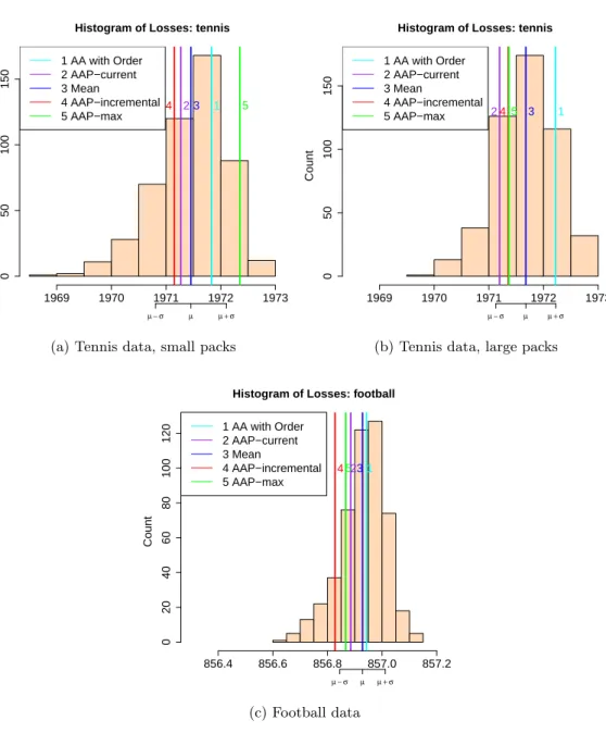
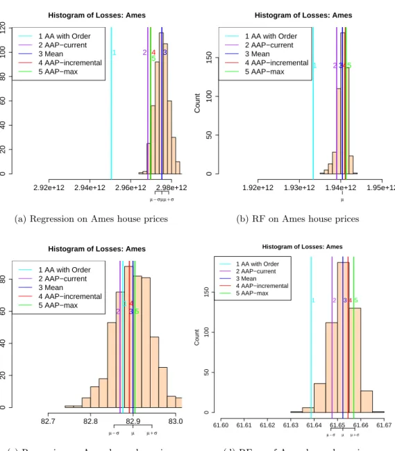
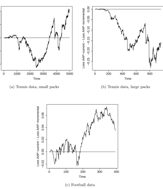
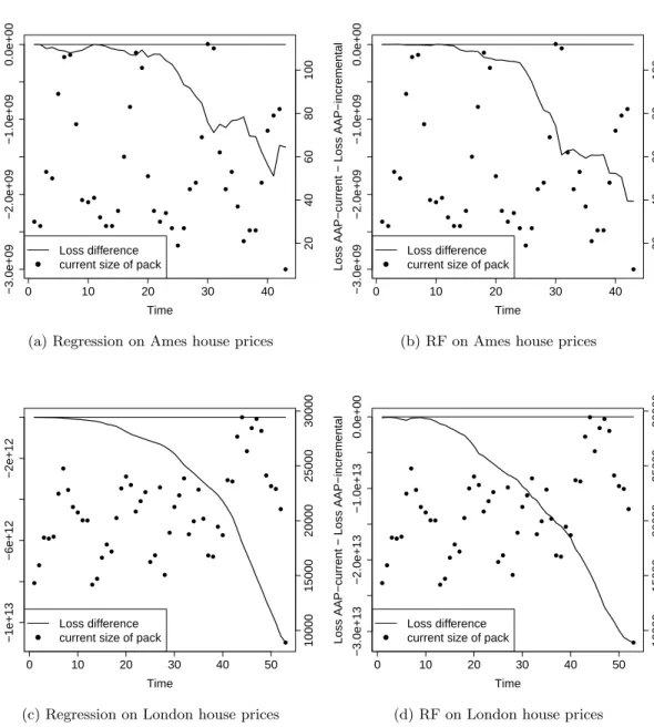
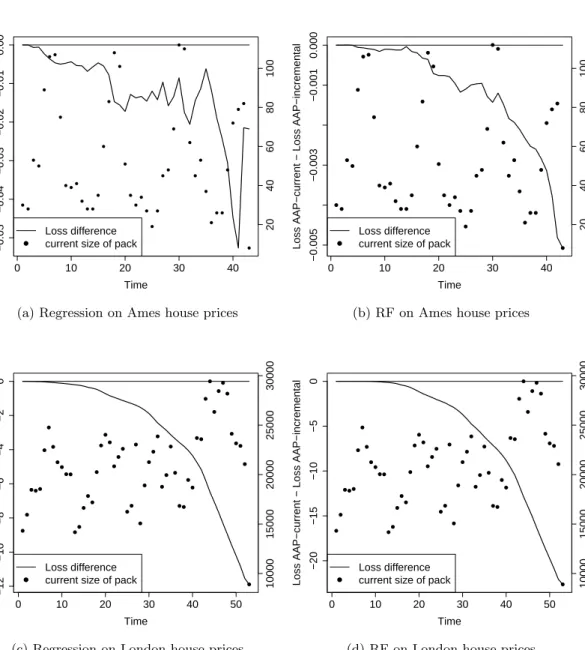
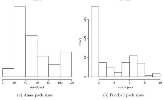
For experiments we predict outcomes of sports matches based on bookmakers’ odds and work out house prices based on descriptions of houses. The sports datasets in-clude football matches, which naturally contain packs, and tennis matches, where we introduce packs artificially in two different ways. The house price datasets contain records of property transactions in Ames in the US and the London area. The datasets only record the month of a transaction, so they are naturally organised in packs. The house price experiments follow the approach of Kalnishkan et al. (2015): prediction with expert advice can be used to find relevant past information. Predictors trained on different sections of past data can be combined in the online mode so that relevant past data is used for prediction.
The performance of the Parallel Copies algorithm depends on the order of outcomes in the packs, while our algorithms are order-independent. We compare the cumulative loss of our algorithms against the loss of Parallel Copies averaged over random permu-tations within packs. We conclude that while Parallel Copies can perform very well, especially if the order of outcomes in the packs carries useful information, the loss of our algorithms is always close to the average loss of Parallel Copies and some algorithms beat the average.
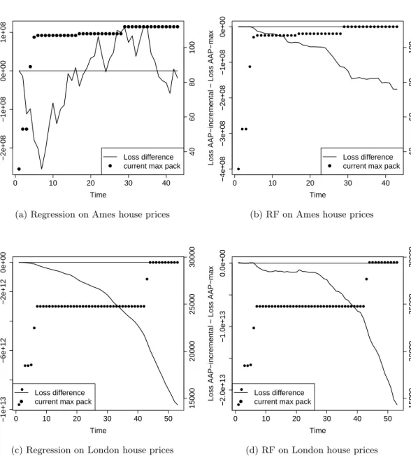
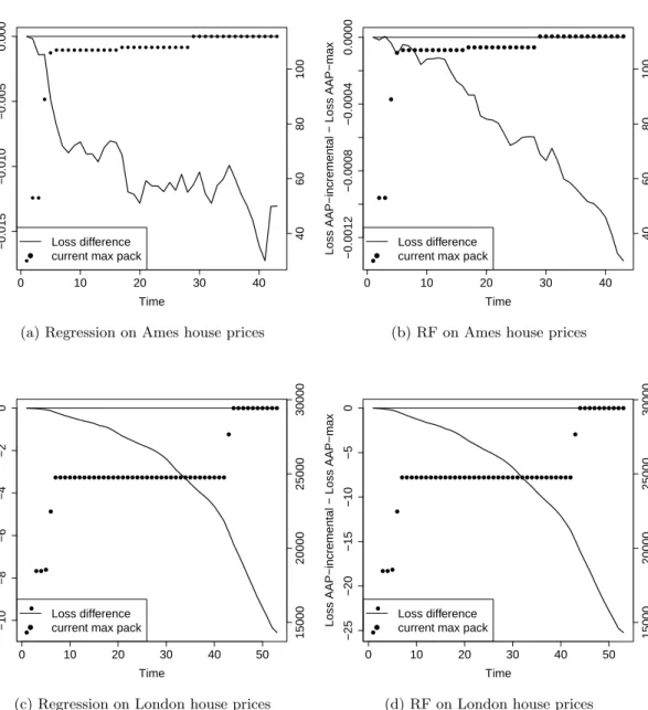
We then compare our algorithms to each other concluding that AAP-max is the worst and AAP-current outperforms AAP-incremental if the ratio of the maximum to the minimum pack size is small.
3.2
Preliminaries and Background
In this section, we introduce the framework of prediction of packs and review connec-tions with the literature.
3.2.1 Protocols for Prediction of Packs
A game G = hΩ,Γ, λi contains an outcome space Ω, prediction space Γ, and loss functionλ: Γ×Ω→[0,+∞].
In the classical protocol, the learner makes a prediction (possibly upon using a signal) and then the outcome is immediately revealed. In this chapter, we consider an extension of this protocol and allow the outcomes to come inpacksof possibly varying size. The learner must produce a pack of predictions before seeing the true outcomes. The following protocol summarises the framework.
Protocol 4 (Prediction of packs).
FOR t= 1,2, . . .
nature announces xt,k∈X, k= 1,2, . . . , Kt
learner outputs γt,k∈Γ, k= 1,2, . . . , Kt
nature announces yt,k ∈Ω, k= 1,2, . . . , Kt
learner suffers losses λ(yt,k, γt,k), k= 1,2, . . . , Kt
ENDFOR
At every trial tthe learner needs to makeKt predictions rather than one. We will be speaking of a pack of the learner’s predictionsγt,k ∈Γ, k = 1,2, . . . , Kt, a pack of outcomes yt,k∈Ω,k= 1,2, . . . , Kt etc.
In this chapter, we assume a full information environment. The learner knows Ω, Γ, and λ. It sees all yt,k as they become available. On the other hand, we make no assumptions on the mechanism generatingyt,k and will be interested in worst-case guarantees for the loss. The outcomes do not have to satisfy probabilistic assumptions such as i.i.d., and can behave maliciously.
Now let E1,E2, . . . ,EN be experts working according to Protocol 4. Suppose that on each turn, their predictions are made available to a learner S as a special kind of side information. The learner then works according to the following protocol.
Protocol 5 (Prediction of packs with expert advice).
FOR t= 1,2, . . .
each expert Ei, i= 1,2, . . . , N, announces
learner outputs predictions γt,k∈Γ, k= 1,2, . . . , Kt
nature announces yt,k ∈Ω, k= 1,2, . . . , Kt
each expert Ei, i= 1,2, . . . , N, suffers
losses λ(yt,k, ξt,k(i)), k= 1,2, . . . , Kt
learner suffers losses λ(yt,k, γt,k), k= 1,2, . . . , Kt
ENDFOR
The goal of the learner in this setup is to suffer loss close to the best expert in retrospect (in whatever formal sense that can be achieved). We look for merging strategies for the learner making sure that the learner achieves low cumulative loss as compared to the experts; we will see that one can quantify cumulative loss in different ways.
The merging strategies we are interested in are computable in some natural sense; we will not make exact statements about computability though. We do not impose any restrictions on experts. In what follows, the reader may substitute the clause ‘for all predictionsξt,k(i)’ appearing in Protocol5for the more intuitive clause ‘for all experts’. There can be subtle variations of this protocol. Instead of getting allKtpredictions from each expert at once, the learner may be getting predictions for each outcome one by one and making its own before seeing the next set of experts’ predictions. For most of our analysis this does not matter, as we will see later. The only thing that matters is that the outcomes come in one go after the learner has finished predicting the pack.
3.2.2 Delayed Feedback Approach
The protocol of prediction with packs can be considered as a special case of the delayed feedback settings surveyed byJoulani et al.(2013).
In the delayed feedback prediction with expert advice protocol, on every step the learner gets just one round of predictions from each expert and must produce its own. However, the outcome corresponding to these predictions may become available later. If it is revealed on the same trial as in Section2.2.1, we say that the delay is one. If it is revealed on the next trial, the delay equals two, etc. Prediction of packs of size not exceedingK can be considered as prediction with delays not exceeding K.
The algorithm BOLD (Joulani et al.,2013) for this protocol works as follows. Take an algorithm working with delays of 1 (or packs of size 1); we will call it the base algorithm. In order to merge experts’ predictions, we will run several copies of the base algorithm. They are independent in the sense that they do not share information. Each copy will repeatedly receive experts’ predictions for merging, output a prediction, and then wait for the outcome corresponding to the prediction. At every moment a
copy of the base algorithm either knows all outcomes for the predictions it has made or is expecting the outcome corresponding to the last prediction. In the former case we say that the copy is ready (to merge more experts’ predictions) and in the later case we say that the copy is blocked (and cannot merge).
At each trial, when a new round of experts’ predictions arrives, we pick a ready algorithm (say, one with the lowest number) and give the experts’ predictions to it. It produces a prediction, which we pass on, and the algorithm becomes blocked until the outcome for that trial arrives. If all algorithms are currently blocked, we start a new copy of the base algorithm.
Suppose that we are playing a gameGandCis admissible forGwith a learning rate η. For the base algorithm take AA with C, η and initial weights p(1), p(2), . . . , p(N). If the delay never exceedsD, we never need more thanD algorithms in the array and each of them suffers loss satisfying inequality (2.10). Summing the bounds up, we get that the loss ofS using this strategy satisfies
LT ≤CLiT +
CD η ln
1
p(i) (3.1)
for every expertEi, where the sum inLT is taken over all outcomes revealed before step
T + 1. The value ofD does not need to be known in advance; we can always expand the array as the delay increases. We will refer to the combination of BOLD and AA in the above fashion as the Parallel Copiesalgorithm.
For Protocol 5described in Section 3.2.1we can define plain cumulative loss
LT = T X t=1 Kt X k=1 λ(yt,k, γt,k) , (3.2) LiT = T X t=1 Kt X k=1 λ(yt,k, ξt,k(i)) , i= 1,2, . . . , N. (3.3) Then (3.1) implies LT ≤CLiT + CK η ln 1 p(i) , (3.4)
whereK = maxt=1,2,...,TKt, forS following Parallel Copies.
However, the Parallel Copies algorithm has two disadvantages. First, it requires us to maintain D arrays of experts’ weights. Each copy of AA needs to maintain N weights, one for each expert. If packs of size Dcome up, we will need D such arrays. Secondly, and more importantly, the algorithm depends on the order of predictions in the pack. It matters what copy of the AA will pick a particular round of experts’ predictions and the result is not invariant w.r.t. the order within the packs.
Below we will build algorithms that are order-independent and have loss bounds both similar (Section 3.4.1) and essentially different (Section 3.4.2) from (3.4). Our method is based on a generalisation of the concept of mixability and a direct application of AA to packs. The resulting algorithms will maintain one array of N weights (or losses).
3.3
Mixability
In this section, we extend the concept of mixability defined in Section2.2.1to packs of outcomes. This will be a key tool for the analysis of the algorithms we will construct. We need upper bound on admissible constants in order to get upper loss bounds and lower bounds in order to establish some form of optimality. As we cannot restrict ourselves to packs of constant size, we need to consider suboptimal constants too.
For a game G=hΩ,Γ, λi and a positive integerK consider the game GK with the outcome and prediction space given by the Cartesian products ΩK and ΓK and the loss function λ(K)((y1, y2, . . . , yK),(γ1, γ2, . . . , γK)) = PKk=1λ(yk, γk). What are the mixability constants for this game? Let Cη be the constants for G and Cη(K) be the constants forGK.
The following lemma provides an upper bound forCη(K).
Lemma 3.3.1. If C >0 is admissible for a game G with a learning rate η >0, then
C is admissible for the game GK with the learning rate η/K.
Proof. Take N predictions in the game GK, ξ(1) = (ξ11, ξ21, . . . , ξ1K), . . . , ξ(N) = (ξ1N, ξN2 , . . . , ξKN) and weights p(1), p(2), . . . , p(N). Since C is admissible for G, there are predictionsγ1, γ2, . . . , γK ∈Γ such that
e−ηλ(yk,γk)/C ≥
N
X
i=1
p(i)e−ηλ(yk,ξki)
for every yk ∈Ω. We will use (γ1, γ2, . . . , γK) ∈ ΓK to show that C is admissible for
GK. Multiplying the inequalities we get
e−ηPKk=1λ(yk,γk)/C ≥ K Y k=1 N X i=1 p(i)e−ηλ(yk,ξki) .
We will now apply the generalised H¨older inequality. On measure spaces (S,Σ, µ) formed by the space S, the σ-field Σ of measurable sets in this space, and the mea-sure µ defined on this σ-field, the inequality states that for all measurable real- or
complex-valued functions f1, . . . , fK defined on S: kQKk=1fkkr ≤QKk=1kfkkrk, where
PK
k=11/rk = 1/r. This follows by induction from the version of the inequality given by (Lo`eve, 1977, Section 9.3). Interpreting a vector xk = (xk(1), xk(2), . . . , xk(N))∈RN
as a function on a discrete space{1,2, . . . , N}and introducing on this space a measure p(i),i= 1,2, . . . , N, we obtain N X i=1 p(i) K Y k=1 xk(i) r!1/r ≤ K Y k=1 N X i=1 p(i)|xk(i)|rk !1/rk .
Lettingrk= 1 and r= 1/K we get
e−ηPKk=1λ(yk,γk)/C ≥ K Y k=1 N X i=1 p(i)e−ηλ(yk,ξik) ≥ N X i=1 p(i)e−PKk=1ηλ(yk,ξik)/K !K .
Raising the resulting inequality to the power 1/K completes the proof.
Remark 1. Note that the proof of the lemma offers a constructive way of solving (2.1)
forGK provided we know how to solve (2.1) for G. Namely, to solve (2.1) forGK with
the learning rateη/K, we solve K systems for Gwith the learning rate η.
We will now show that the admissible constants given by Lemma 3.3.1cannot be decreased for a wide class of games.
Lemma 3.3.2. Let a game G have a convex set of superpredictions. If C > 0 is
admissible for GK with a learning rate η/K > 0, then C is admissible for G with the
learning rate η.
The requirement of convexity is not too restrictive. For a wide class of games the following implication holds. If the game is mixable (i.e., Cη = 1 for someη >0), then its set of superpredictions is convex. (Kalnishkan et al., 2004, Lemma 7) essentially prove this for games with finite sets of outcomes.
Proof. Since C >0 is admissible forGK with the learning rate η/K >0, for everyN
arrays of predictions ξ(1) = (ξ11, ξ12, . . . , ξK1), . . . , ξ(N) = (ξ1N, ξ2N, . . . , ξKN) and weights p(1), p(2), . . . , p(N) there areγ1, γ2, . . . , γK ∈Γ such that
K X k=1 λ(yk, γk)≤ − C η/Kln N X i=1 p(i)e−ηPKk=1λ(yk,ξik)/K
for all y1, y2, . . . , yK ∈Ω.
GivenN predictions ξ1, ξ2, . . . , ξN ∈Γ, we can turn them into predictions from ΓK by considering N arrays ξ(i) = (ξi, . . . , ξi) ∈ ΓK, i= 1,2, . . . , N. By the above there are predictionsγ1∗, γ2∗, . . . , γK∗ ∈Γ satisfying
1 K K X k=1 λ(y, γk∗)≤ −C η ln N X i=1 p(i)e−ηλ(y,ξi)
for all y∈Ω (we let y1=y2 =. . .=yK =y).
We have found a prediction from ΓK, but we need one from Γ. The problem is thatγk∗do not have to be equal. However,PK
k=1λ(y, γ ∗
k)/K is a convex combination of superpredictions w.r.t. G. Since the set of superpredictions is convex, this expression is a superprediction and there is γ ∈ Γ such that λ(y, γ) ≤ PK
k=1λ(y, γk∗)/K for all
y∈Ω.
SinceCη andCη/K(K) are the infimums of admissible values, Lemma3.3.1and Lemma
3.3.2can be combined into the following theorem.
Theorem 3.3.3. For a game G with a convex set of superprediction, any positive integer K and learning rate η >0, we haveCη/K(K) =Cη.
This theorem allows us to merge experts’ predictions in an optimal way for the case when all packs are of the same size. In this case, we simply apply Proposition2.10and all the existing theory of the AA to the gameGK.
In order to analyse the case when pack sizes vary, we need to make a simple obser-vation on the behaviour ofC(K1)
η/K2 forK1≤K2.
Lemma 3.3.4. For every gameG, if C >0 is admissible with a learning rate η1 >0,
it is also admissible with every η2≤η1. Hence the value of Cη is non-decreasing in η.
Proof. Raising the inequality
e−η1λ(y,γ)/C ≥
N
X
i=1
p(i)e−η1λ(y,ξ(i))
to the powerη2/η1 ≤1 and using Jensen’s inequality we get
e−η2λ(y,γ)/C ≥ N X i=1 p(i)e−η1λ(y,ξ(i)) !η2/η1 ≥ N X i=1 p(i)e−η2λ(y,ξ(i)) .
Corollary 2. For every game G and positive integers K1 ≤ K2, we have C (K1)
η/K2 ≤
C(K1)
η/K1.
Proof. The proof is by applying Lemma 3.3.4toGK1.
Remark 2. The proofs of the lemma and corollary are again constructive in the
fol-lowing sense. If we know how to solve (2.1) for G with a learning rate η1 and an
admissibleC, we can solve (2.1) for η2 ≤η1 and the same C.
Suppose we play the game GK1 but have to use the learning rateη/K2, whereK2 ≥
K1, withC admissible forG withη. To solve (2.1), we can take K1 solutions for (2.1)
for G with the learning rate η.
3.4
Algorithms for Prediction of Packs
In this section, we apply the theory we have developed to obtain prediction algorithms. This can be done in two essentially different ways leading to different types of bounds. In Section3.4.1we introduce AAP-max and AAP-incremental, and in Section3.4.2we introduce AAP-current.
3.4.1 Prediction with Plain Bounds
Consider a gameG={Ω,Γ, λ}. TheAggregating Algorithm for Packs with the Known
Maximum(AAP-max) and theAggregating Algorithm for Packs with an Unknown
Max-imum (AAP-incremental) take as parameters a prior distribution p(1), p(2), . . . , p(N) (such thatp(i)≥0 andPN
i=1p(i) = 1), a learning rateη >0 and a constantC admis-sible forη. AAP-max also takes a constantK >0. The intuitive meaning is thatK is an upper bound on pack sizes, Kt≤K.
The algorithms follow very similar protocols and we will describe them in parallel. The algorithm AAP-max works as follows.
Protocol 6 (AAP-max).
1 initialise losses Li0= 0, i= 1,2, . . . , N
2 this step is skipped
3 set weights to w0(i) =p(i), i= 1,2, . . . , N
4 FOR t= 1,2, . . .
5 normalise the weights pt−1(i) =wt−1(i)/PNi=1wt−1(i)
6 FOR k= 1,2, . . . , Kt
7 read the experts’ predictions ξt,k(i), i= 1,2, . . . , N
inequality λ(y, γt,k)≤ −Cη lnPNi=1pt−1(i)e−ηλ(y,ξt,k(i))
9 ENDFOR
10 observe the outcomes yt,k, k= 1,2, . . . , Kt
11 update the losses Lit=Lit−1+PKt
k=1λ(yt,k, ξt,k(i)),
i= 1,2, . . . , N
12 let Kmaxt =K
13 update the experts’ weights wt(i) =p(i)e−ηL
i t/K t+1 max, i= 1,2, . . . , N 14 END FOR
The algorithm AAP-incremental follows a protocol that is the same except for the following lines:
Protocol 7 (AAP-incremental).
2 initialise K0
max= 1
12 update Kmaxt = max(Kmaxt−1, Kt)
As AAP-max always uses the same K for calculating the weights, line 13 can be replaced with an equivalent
wt(i) =wt−1(i)e−η PKt
k=1λ(yt,k,ξt,k(i))/K
and losses do not need to be maintained explicitly.
If C is admissible for G with the learning rate η and pt−1(i), i = 1,2, . . . , N, the step on line 8 can always be performed and the (plain) cumulative losses (3.2) and (3.3) satisfy the following inequalities.
Theorem 3.4.1. Let C be admissible for G with the learning rateη. Then 1. The learner following AAP-max suffers loss satisfying
LT ≤CLiT +
KC η ln
1 p(i)
for all outcomes and experts’ predictions as long as the pack size does not exceed
K, i.e., Kt≤K, t= 1,2, . . . , T.
2. The learner following AAP-incremental suffers loss satisfying
LT ≤CLiT +
KC η ln
1 p(i) ,
where K is the maximum pack size overT trials,K = maxt=1,2,...,T+1Kt, for all
outcomes and experts’ predictions.
The theorem provides an alternative of Lemma2.2.3for the prediction of packs. The bounds are similar to the bound for the AA except that the regret term is multiplied by the maximum pack sizeK. For mixable games the theorem states that for a finite number of experts the AAP-max and AAP-incremental predict as well as the best expert up to an additive constant.
Proof. The proof essentially repeats that of Proposition 2.10. By induction one can
show that e−ηLT/(CKmaxT )≥ N X i=1 p(i)e−ηLiT/KmaxT . (3.5)
Line 8 of Protocols 6and 7 ensure that inequality (3.5) holds for T = 1.
Assume that (3.5) holds. We first raise inequality (3.5) to the powerKmaxT /KmaxT+1 ≤
1 and apply Jensen’s inequality:
e−ηLT/(CKmaxT+1)≥ N X i=1 p(i)e−ηLiT/KmaxT !KmaxT /KmaxT+1 ≥ N X i=1 p(i)e−ηLiT/K T+1 max . (3.6)
According to line 8 of Protocols 6and 7 we have that
e− η KmaxT+1 PKT+1 k=1 λ(yT+1,k,γT+1,k)/C ≥ N X i=1 pT(i)e − η KTmax+1 PKT+1 k=1 λ(yT+1,k,ξT+1,k(i)) = PN i=1p(i)e −ηLi T+1/K T+1 max PN i=1p(i)e−ηL i T/K T+1 max . (3.7)
By multiplying inequalities (3.6) and (3.7), we get (3.5).
To complete the proof, it remains to drop all terms from the sum in inequality (3.5) except for one.
3.4.2 Prediction with Bounds on Pack Averages
The Aggregating Algorithm for Pack Averages (AAP-current) takes as parameters a
prior distributionp(1), p(2), . . . , p(N) (such thatp(i)≥0 andPN
i=1p(i) = 1), a learning rateη >0 and a constantC admissible for η.
Protocol 8 (AAP-current).
2 FOR t= 1,2, . . .
3 normalise the weights pt−1(i) =wt−1(i)/PNi=1wt−1(i)
4 FOR k= 1,2, . . . , Kt
5 read the experts’ predictions ξt,k(i), i= 1,2, . . . , N
6 output γt,k ∈Γ satisfying for all y∈Ω the
inequality λ(y, γt,k)≤ −Cη ln
PN
i=1pt−1(i)e
−ηλ(y,ξt,k(i))
7 ENDFOR
8 observe the outcomes yt,k, k= 1,2, . . . , Kt
9 update the experts’ weights wt(i) =wt−1(i)e−η
PKt
k=1λ(yt,k,ξt,k(i))/Kt,
i= 1,2, . . . , N
10 END FOR
In line 9 we divide by the size of the current pack.
Defining cumulative average loss of a strategy S and experts Ei working in the environment specified by Protocol4as
Laverage,T = T X t=1 PKt k=1λ(yt,k, γt,k) Kt , Liaverage,T = T X t=1 PKt k=1λ(yt,k, ξt,k(i)) Kt , i= 1,2, . . . , N,
we get the following theorem.
Theorem 3.4.2. If C is admissible for G with the learning rate η, then the learner following AAP-current suffers loss satisfying
Laverage,T ≤CLiaverage,T +
C η ln
1
p(i) (3.8)
for all outcomes and experts’ predictions.
The bound (3.8) coincides with the bound for the AA in Lemma 2.2.3. However, note that the bound for the AAP-current is provided on the cumulative average loss instead of the cumulative loss. For mixable games the theorem states that for a finite number of experts the AAP-current predicts as well as the best expert up to an additive constant in terms of the cumulative average loss.
Proof. We again prove by induction that
e−ηLaverage,T/C ≥
N
X
i=1