Privacy-preserving statistical analysis methods and their applications on health research

(1)

Privacy-Preserving Statistical Analysis Methods

and their Applications on Health Research

by

c

Ahoora Sadeghi Boroujerdi

A thesis submitted to the

School of Graduate Studies

in partial fulfilment of the

requirements for the degree of

Master of Computer Science

Department of Computer Science

Memorial University of Newfoundland

October 2016

(2)

Abstract

Privacy consideration in health data usually prevents researchers and other data

users from conducting their research. Also, data is distributed through various health

organizations such as hospitals, thus gathering distributed health information

be-comes impractical. Various approaches have been proposed to preserve the patients

privacy, whilst allowing researchers to perform mathematical operations and

statisti-cal analysis methods on health data, such as anonymization and secure computation.

Data anonymization reduces the accuracy of the original data; hence the final

re-sult would not be precise enough. In addition, there are several known attacks on

anonymized data, such as using public information and background knowledge to

re-identify the original data. On the other hand, secure computation is more precise

and the risk of data re-identification is zero; however, it is computationally less

effi-cient than data anonymization. In this thesis, we implemented a web-based secure

computation framework and propose new secure statistical analysis methods. Using

the proposed web application, researchers and other data users would be able to

per-form popular statistical analysis methods on distributed data. They will be able to

perform mathematical operations and statistical analysis methods as queries through

different data owners, and receive the final result without revealing any sensitive

in-formation. Digital Epidemiology Chronic Disease Tool (DEPICT) database, which

contains real patients information, will be used to demonstrate the applicability of

the web application.

Keywords Secure Multiparty Computation; Web-Based Framework, Privacy-Preserving; Homomorphic Encryption, Secure Statistical Analysis Methods

(3)

Acknowledgements

First, I would like to thank my mentor and supervisor Dr. Saeed Samet. Prof.

Samet was always there for me and was always helpful and understanding when I ran

into a problem or have a question about my research. I would have not been able to

do this research if it was not for him. He allowed me to work on the research on my

own, but guided me on the right direction whenever I needed it.

I would also like to thank the experts who were involved and contributed in this

research: Dr. Shabnam Ashghari, Dr. Gerard Farrell and Mr. Oliver Hurley for their

thoughtful comments, suggestions and contributions.

I thank all my friends for their continuous support through all the challenges that

I faced throughout my academic life at Memorial University of Newfoundland.

I consider myself the luckiest person for having the best wife anyone can think

of. I can not think of any words to express my very profound gratitude towards my

wife, Nadia. Her strength, love and understanding gave me everything that I needed

throughout my years of study. This accomplishment would not have been possible

without her. Thank you.

Last but not least, I would like to thank my family: my parents and my brothers

for encouraging me to continue my study towards Masters and for supporting me

(4)

List of Tables

1 2x2 Contingency Table . . . 8

2 Performance Results for the Pre-processing Stage . . . 86

3 Performance Results for the Cryptosystem and Secure Addition . . . 86

4 Performance Results for the Protocols Including Fetching Data from

Database . . . 87

5 Performance Results for the Protocols when Data is Stored in Memory 87

6 Secure Protocols Performances with no conditions and 10000 records 89

7 Secure Protocols Performances with no conditions and 100000 records 89

8 Secure Protocols Performances with conditions and 10000 records . . 90

(8)

List of Figures

1 k-anonymity example . . . 19

2 Clifton secure sum protocol . . . 23

3 subset data distribution . . . 26

4 partial data distribution . . . 27

5 Orocess Flow of the Protocol . . . 33

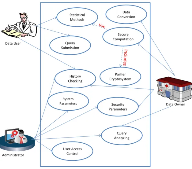
6 Use Case Diagram . . . 55

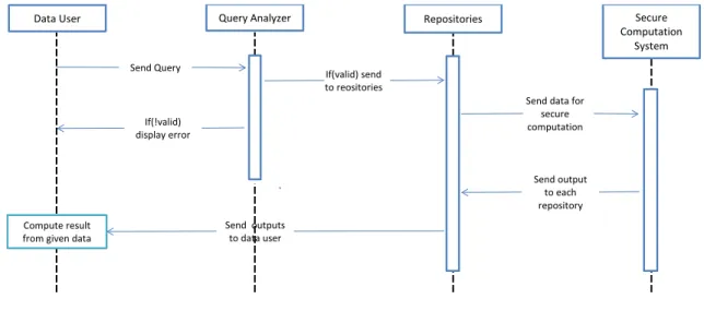
7 Sequence Diagram . . . 56

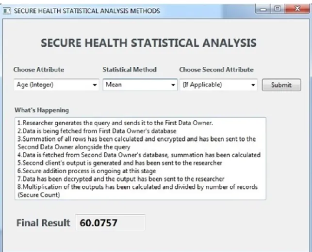
8 Desktop Application . . . 57

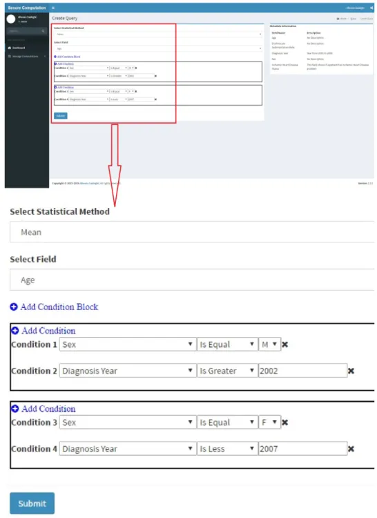
9 Mean Query Page . . . 79

10 Mean Query Result . . . 80

11 Correlation Query Page . . . 81

12 Correlation Query Result . . . 82

13 Linear Regression Query Page . . . 83

14 Linear Regression Query Result . . . 84

15 registration use case diagram . . . 105

(9)

17 key generation use case diagram . . . 107

18 query submission use case diagram . . . 108

19 secure computation database scheme . . . 109

(10)

Chapter 1 Introduction

Preserving the security and privacy of health information plays an important role in

the modern era. Technology grows every day and the need to protect confidential

data has become essential. At the same time, researchers and scientists should be

able to access these data for research purposes, to execute mathematical operations or

statistical analysis methods on data. For many years, researchers had to physically

go to health data centers in order to conduct their research. This is still a

com-mon practice; however, two settings introduced for privacy-preserving have brought

more options to make this process easier. The first approach is anonymization and

randomization such as generalization, suppression, and random sampling, and the

second one is secure (multi-party) computation. There are various approaches for

data anonymization such as optimal k-anonymization [7] and fast data

anonymiza-tion [27]. When anonymizaanonymiza-tion is used, no confidential data is revealed and statistical

methods can be executed. The results taken from de-identified data are not precise

(11)

Secure computation leads to more precise and secure results; therefore, researchers

would be able to perform their own statistical methods on the data without revealing

any confidential information. The risk of re-identification is close to zero, but it could

be computationally prohibitive comparing to performing statistical analysis methods

on anonymized data.

Andrew Yao [64] introduced the concept of secure computation in 1982. The idea

was to perform a function on two parties’ private data, and only return the result

to each party (or a third party) without revealing any other information from one

to the other. Not long after, Yao’s approach was generalized by Goldreich, Micali

and Wigderson for multiple parties [29]. This means that instead of only two parties,

more than two parties (n where n≥3) parties can participate.

Secure computation guarantees that no sensitive information would be revealed, but

allows the end-users to perform a function on their private data. Secure computation

can be done using various approaches, and several implementations of secure

com-putations have been proposed and developed in recent years [37, 5]. Also, various

privacy-preserving protocols with diverse functionalities have been built based on the

above approaches. In addition, cryptography techniques, such as homomorphic

en-cryption, could be used for secure computation. There are two types of homomorphic

encryption systems; partially homomorphic cryptosystems such as Paillier [46],

Elga-mal [22], and RSA [48], and fully homomorphic encryption systems such as the work

proposed by Gentry [26].

Ideally, any mathematical operation can be performed on encrypted data using fully

homomorphic cryptosystems. Gentry [26] proposed the most popular fully

(12)

does not live up to other cryptosystems, which makes it impractical for long

mes-sages. However, not all mathematical operations can be performed using partially

homomorphic encryption systems. Gentry [26] scheme supports both addition and

multiplication operations and is based on somewhat homomorphic encryption scheme.

This is still impractical when the security level increases. Cramer et al. [14] scheme

is based on homomorphic threshold cryptosystem, which can be used for multi-party

computation, but there is an issue with their approach. Long messages cannot be

split, because the chosen ciphertext property is not preserved in this way. Domingo

Ferrer [18] proposed another homomorphic encryption scheme, but the ciphertext

message space is too large and is impractical for long messages. Although fully

homo-morphic encryption systems are making huge improvements for secure computation,

no practical approach has been proposed yet. When dealing with sensitive data such

as health information, there are many factors to consider other than the security of

the system such as the usage and disclosure of personal health information.

Personal health information is a sensitive type of personal information that can be

shared for multiple purposes such as research, treatment and care. The collection, use

and disclosure of personal health information has been addressed by different privacy

acts such as Personal Health Information Act (PHIA) and Personal Health

Informa-tion ProtecInforma-tion Act (PHIPA). These acts consists of sets of rules in which all data

custodians, individuals, agents, and health organizations should follow. Every person

who delivers healthcare services or product should follow defined rules. There exists

seven categories in the definition. Under this act, each individual or organization that

provides technology to a data custodian, must follow the restrictions on how to use

(13)

are the recipient of personal health information, must follow the act. The act

pro-tects personal health information in oral or written form that are related to a person’s

physical or mental health, identification, payment related to healthcare and other

in-formation that are related to an individual’s inin-formation. These rules restrict and

prevent health organizations to share their information for research purposes. Also,

health organizations usually resist on sharing information for security and beneficial

reasons, but they are willing to provide secure services in order to get an aggregated

result.

A practical and secure solution has been introduced by Samet et al. [51], in which

data owners could securely and jointly perform a privacy-preserving protocol by only

exchanging encrypted values between themselves. At the end, each of them will send

their portion of the final results to the researcher to combine the received shares and

construct the final results of their query. In this thesis, we focus on implementing a

web-based framework based on various works done by Samet such as [52, 53, 50, 51],

which can be improved by adding more statistical analysis methods modified for

multi-party computation. Various features have been added to this framework, such

as including an authorized server for user access control or system parameterization.

The outline of this thesis is as follow: Chapter 2 covers basic definitions and

pre-liminaries. In Chapter 3, we review background and related work. The proposed

approach, research methods and various aspects of the system such as configurations

are discussed in Chapter 4. In Chapter 5, we thoroughly explain the implementation

of the web-based framework, system parameters, and features. Experimental results

will be covered and shown in Chapter 6, followed by conclusions and future work in

(14)

Chapter 2 Preliminaries and Definitions

In this chapter, we will describe the terminologies, techniques, and concepts used in

our system to make sure that reader will have basic understanding of our system

design.

2.1 Statistical Analysis Methods

Statistical analysis is the science of collecting, interpreting and presenting large

amount of data to find out about the existing patterns and trends. Statistical

anal-ysis is fundamental to all researches that use statistics as a methodology. In social

sciences, engineering, healthcare and many other fields, statistics are applied every

day. There exists various statistical analysis methods such as arithmetic mean,

vari-ance, standard deviation, student’s t-test, linear regression and logistic regression. Therefore, each can be used to interpret data in a unique way. Some of statistical

(15)

1. Mean: The arithmetic mean is an average score which is the sum of individual scores divided by the number of those individuals. If our sample data consists

of values x1, x2,· · · , xn, mean (denoted by ¯x) is as below: ¯

x= (x1+x2+· · ·+xn)

n (2.1)

2. Standard Deviation [9]: Standard deviation is to measure the dispersion or deviation of a set of data from its mean and is a measure of the spread of

scores. To calculate standard deviation, variance has to be calculated first and

the square root of variance is standard deviation. Variance is also a method to

measure the spread between numbers in a data set. To calculate the variance,

the differences between each number in the data set and the mean is measured

and squared. Then the summation of these values is calculated and divided

by the number of the values in the set. If our sample data consists of values

x1, x2,· · · , xn, variance (denoted by σ2) is as below: σ2 = n P i=1 (xi−x)¯ 2 n (2.2)

Thus, standard deviation (denoted by σ) is:

σ =√σ2 ₌ v u u t n P i=1 (xi−x)¯ 2 n (2.3)

3. Skewness [41]: When the normal distribution of a set of data is measured, the distribution might have fewer data on the right or the left, which is said that the

(16)

calculate the asymmetry of a set of data in normal distribution. If our sample

data consists of values x1, x2,· · · , xn, skewness (denoted by γ) is as below:

γ = n P i=1 (xi−x)¯ 3 nσ3 (2.4)

4. Correlation [24]: Correlation is a statistical method to measure how strong two sets of variables are linked. Also, it can be used to measure the movement

(increase or decrease) of the second variable when the first variable moves.

Correlation ranges between−1 and +1. When correlation is positive, it can be

implied that the sets of variables move in the same direction (increase or decrease

together). Also, when correlation is negative, it shows that the variables move in

the opposite direction (when one increases, the other decreases). If our sample

data consists of values x1, x2,· · · , xn for the first variable and y1, y2,· · · , yn for the second variable, correlation (denoted by ρ) is as below:

ρ= ( n P i=1 xi ∗yi)−n∗x¯∗y¯ n∗σx∗σy (2.5)

5. Chi-Square Test[40]: Chi-Square is a test to compare the observed data with the expected result according to a hypothesis. Also, it can be used to view the

distribution differences between categorical variables. Thus, the variables’ types

should be categorical such as ”yes” and ”no” or ”0” and ”1”. For simplicity of

the mentioned method, we imagine a 2x2 contingency table for two categorical

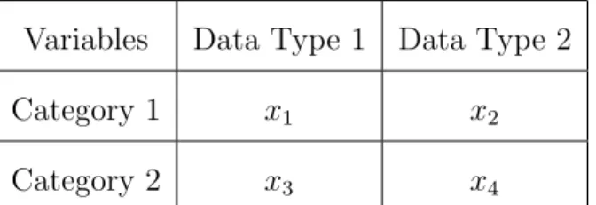
variables and two data types. The contingency table is shown in Table 1.

(17)

Variables Data Type 1 Data Type 2

Category 1 x1 x2

Category 2 x3 x4

Table 1: 2x2 Contingency Table

is as below: χ2 = (x1∗x4−x2∗x3) 2_∗_(x 1∗x2∗x3∗x4) (x1+x2)∗(x3+x4)∗(x2+x4)∗(x1 +x3) (2.6)

Whenχ2is close to zero, we denote that there is no significant difference between the observed result and the expected result.

6. Student’s t-test [56]: A t-test is an examination of two samples’ means. In students t-test, both samples should follow the normal distribution if the null hypothesis is true and examines the difference between two samples. It is mostly

used when there are two variables and one of them is a measurement variable

and the other is a categorical variable. For a sample of size n with mean value

of ¯x1 and standard deviation σ drawn from a random population with mean

value of ¯x2 and unknown standard deviation, Student’s t-test (denoted byt) is

as below:

t= x¯1−x¯2

σ_/√_n (2.7)

In student’st-test, the degree of approximation depends on parent’s population closeness to normal distribution and also on the sample size.

7. Linear Regression[45]: Linear regression is a predictive analysis to model the relationship between two variables where one variable is a dependent variable

(18)

and the other variable is independent. Linear regression finds a linear function

that fits a given set of data points in the dataset that best describes the bivariate

data. IfX is the independent variable andY is the dependant variable, a linear

regression line equation is as below:

Y =a+bX (2.8)

whereais a constant value whenx= 0 andb is the regression coefficient. When

xis the value of an independent variable, the predicted value (denoted by ˆy) is

as below:

ˆ

y =a+bx (2.9)

a and b are calculated as below:

b= n P i=1 (xi−x)(yi¯ −y)¯ n P i=1 (xi−x)¯ 2 (2.10) a= ¯y−b∗x¯ (2.11)

8. Logistic Regression [33]: Logistic regression is a statistical method to model the relationship between one dependant variable which is dichotomous and one

or more independent variable(s). Logistic regression can be described as a

special case for generalized linear model which is based on different assumptions

than linear regression. Unlike linear regression that is used for both continuous

(19)

2.2 Statistical Analysis Methods on Health

Re-search

Statistical methods have plenty of utilizations such as healthcare resources and cost

analysis [43], quality improvement [23], health assessment [6] and many other

applica-tions. As an example, we can simplify the outpatient clinic problem discussed in [23].

The management of an outpatient clinic was notified that the average time between

the patient arrival and the blood test or electrocardiogram (ECG) of the patient is

around 30 minutes. The management decided to monitor the average waiting time of

patients in each day of the week for several weeks. Afterwards, the mean and standard

deviation of the waiting time was calculated for each day of the week. By comparing

the calculated values for each day, they found out that the average waiting time of

the patients on Friday is a lot more than the other days. Thus, they monitor the

patients on Friday and found out that the there are more ECG patients on Fridays

than blood test patients comparing other days of the week. ECG patients require

more examination time than blood test patients. Thus, the average waiting time

on Fridays was significantly more than the other days. Based on the given analysis,

the management decided to dedicate more doctors and nurses on Fridays for ECG

patients and as a result the average waiting time of patients reduced to 15 minutes.

(20)

2.3 Homomorphic Encryption

In algebra, homomorphism is a map between two groups respecting the structure of

each group. A group is a set that includes a law and an operation (4). Assuming we

have two groups such as (G,4) and (H,◦) where 4 and ◦ represent operations on

setG and H respectively, a group homomorphism from G toH is defined as below:

f(a4b) = f(a)◦f(b),

where f is a function from G toH for all a and b in G. Homomorphic encryption is

a type of encryption that allows specific types of computations on the plaintext to

be carried on the ciphertext. If we assume that the plaintexts and ciphertexts create

two homomorphism groups such as (P,4) and (C,◦) respectively, we have:

E(a)4E(b) = E(a◦b),for all a and b inP (2.12)

It also allows computations to be performed on encrypted data without revealing

confidential information about the original data. However, if the private key gets

compromised, data can be leaked by decrypting the encrypted values. There are two

types of Homomorphic Encryption systems: Fully Homomorphic and Partially

Ho-momorphic cryptosystems. A cryptosystem is called a fully hoHo-momorphic encryption

system if it supports arbitrary number of operations such as multiplication and

ad-dition to implement any functions that are needed. Gentry cryptosystem [26] is the

first practical fully homomorphic cryptosystem which supports both multiplication

and addition. Partially homomorphic cryptosystems only support one operation such

as addition or multiplication. There are several partially homomorphic

(21)

cryptosystem [46] which supports addition. In addition, there exist somewhat

ho-momorphic encryption systems. These cryptosystems support a limited number of

operations. Fully homomorphic cryptosystems such as Gentry cryptosystem [26] have

tremendous overhead and other approaches are not practical. Thus, somewhat fully

homomorphic encryption systems such as Brakerski’s scheme [11] which is based on

the ring learning with errors assumption could be used for most of the problems

that do not need an arbitrary number of computations. Many works have been done

in somewhat fully homomorphic encryption field for secure multi-party computation

such as Damgard et al. [15] multi-party computation from somewhat homomorphic

encryption and Boneh et al. [10] private database queries using somewhat

homo-morphic encryption. Most of the mentioned encryption systems are not practical or

secure enough for multi-party computations. Also, the encrypted data is a pair of

numbers which makes fully homomorphic encryption systems more complicated and

impractical to use. Paillier cryptosystem is secure against chosen plaintext attack.

Also, Paillier encryption uses randomness in its encryption method which produces

different ciphertexts for the same plaintext. Because Paillier is an additive

homomor-phic encryption system, we are unable to implement most of the statistical analysis

methods. Thus, we use method proposed in [53] for secure multiplication and the

method of [28] for secure dot product to empower Paillier cryptosystem with various

(22)

2.4 Paillier Cryptosystem

Paillier cryptosystem named after Pascal Paillier is a modular public key scheme

which is also an additive homomorphic cryptosystem. Like any other public key

scheme, it has its own key generation phase, encryption phase using public keys and

decryption phase using private keys. Key generation is as follow:

1. To construct public keys, two randomly generated large prime numbers p, q are

needed. For simplicity, these two numbers can have equal length.

2. Then we calculate their product such that:

n=p∗q (2.13)

3. We also calculate the least common multiple of p−1 andq−1 such that:

λ=lcm(p−1, q−1) (2.14)

4. A random integer g should be selected from Zn2. To ensure that g is divisible

byn, the relationship described by the below equation should hold between the

chosen and used variables:

µ= (L(gλ mod n2))−1(mod n) (2.15)

where Lis a function such that:

L(u) = u−1

n (2.16)

5. The public keys are n and g.

(23)

After generating public keys and private keys, we will be able to encrypt and decrypt

a message and ciphertext respectively. The encryption process is as follow:

1. We choose message m fromZn.

2. Then we select a random number r fromZ_n∗ (Z_n∗ being the invertible elements

of Zn).

3. Encrypting a message is as follow:

c=E(m) = gm∗rn (mod n2) (2.17)

The decryption process would be as follow:

1. We assume that ciphertext c is from Z_n∗2 and previously created by the

cryp-tosystem (it ensures us thatc is invertible inZ_n∗2).

2. Decrypting the ciphertext is as follow:

m=D(c) = L(cλ mod n2)∗µ (mod n2) (2.18) Here is an example of Paillier Cryptosystem. For ease of calculations, small prime

numbers will be chosen for this purpose. Suppose we choose p= 13 and q = 11 for

our prime numbers. Thus, n = 13∗11 = 143. Furthermore, we have to choose a

randomg and calculate λ and µas below:

g = 67, λ=lcm(12,10) = 60, µ = (L(6760 mod 20449))−1 mod 143 = 124 (2.19)

For example, we want to encrypt 7 as our message. First we have to select a random

number and then encrypt the message as below:

(24)

Now we want to decrypt a ciphertext such as 14271. The process is as below:

(25)

Chapter 3 Related Work

Many privacy-preserving techniques tend to transform information in order to

pre-serve privacy. These methods reduce the accuracy of the data and cause information

loss. Randomization and anonymization are some examples of transformation

meth-ods. Randomization is done by adding noise components to the original data in a

way that the variance of the added noise is large enough. By adding noise, original

data cannot be derived from distorted data. Randomization has been used for data

distortion and found its way to privacy preserving in data mining [5]. Noise can be

added to the values in database such as the method proposed by Traub and

Yem-ini [58] in a way that each vector in database is replaced by another vector which

creates a random perturbated vector. Also, noise can be added to the final result

of the query such as the method proposed by Beck [8]. Although randomization is

relatively simple and no knowledge is needed for the distribution of data, it is more

vulnerable to adversarial attacks [2]. More noise should be added to the original data

(26)

accuracy of the data for data mining purposes. In the past, many data owners

cre-ated statistical databases using randomization techniques for research purposes [63].

However, creating statistical databases became time consuming and costly due to

tremendous increase in demand for person-specific data for various applications such

as data mining and fraud detection. Moreover, adding noise to these databases for

preserving the privacy led to inaccurate results.

Data anonymization is the process of de-identifying sensitive data in order to

pro-tect data without any change to the data type. One of the popular techniques for

anonymization is inference in multi-level databases [44]. In multi-level database, the

data is restricted in a way that only lower classified information will be released in

a way that higher classified information could not be revealed. In a more advance

approach which was proposed by Denning and Lunt [17], multiple security

classifica-tions could be defined for multiple types of users and multilevel databases could be

created for each security classification.

In 1999, Agrawal [4] mentioned that an important field of future research could be

the development of techniques to overcome privacy concern. In 2000, Agrawal and

Srikant [5] proposed a method for privacy preserving in the data mining field. The

idea was to let users provide a value for sensitive fields using Value-Class

Member-ship method or Value Distortion method and reconstructing the original distribution.

In their method, the values for an attribute are classified into different groups in a

way that they are mutually exclusive. So, by using discretization some intervals are

created where each value can be stored in a specific interval. In this way, true value

does not have to be stored in the database. For example, age may be discretized into

(27)

and more than 50. By using this discretization, true values for each attribute will

be hidden. Also, values can be distorted instead of being classified. A truly random

number will be added to each value in order to prevent snoopers from estimating

the true value through multiple queries. The random value can be generated using

Uniform Distribution or Gaussian Distribution. It has been shown that

discretiza-tion is less efficient than distribudiscretiza-tion [5]. In order to have the same level of privacy

using discretization comparing to uniform distribution, interval width should be

in-creased significantly which results in inaccurate model. Also, it has been shown that

the Gaussian distribution provides more privacy at higher confidence level compared

to uniform distribution [5]. Thus, the Gaussian distribution has been used in their

approach. In this system, the original distribution should be reconstructed in order

to be useful. The original data distribution can be reconstructed using decision tree

classification over randomized data as shown in [5].

In modern era, data is distributed through various data owners and also there is

re-dundancy between many data owners, thus data owners have incomplete knowledge

over one another. As a result, releasing information without proper knowledge of

other released data may cause revealing sensitive information. Also, suppression is

used for designing multilevel databases which can reduce the quality of the final

re-sult.

Another technique for data anonymization is k-anonymity, which was introduced by

Sweeney [57] in 2002. K-anonymity would guarantee that each record of a data table

is similar to at least k-1 other records on the data table (in terms of Quasi-identifiers).

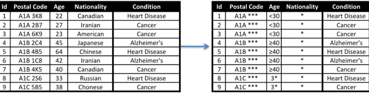
An example of k-anonymity is shown in Figure 1. There are two common methods

(28)

spe-cific attribute will be removed completely. In generalization, the values of a spespe-cific

attribute are generalized to a range. K-anonymity reduces the risk of information

Id Postal Code Age Nationality Condition Id Postal Code Age Nationality Condition

1 A1A 3K8 22 Canadian Heart Disease 1 A1A *** <30 * Heart Disease

2 A1A 2B7 27 Iranian Cancer 2 A1A *** <30 * Cancer

3 A1A 6K9 23 American Cancer 3 A1A *** <30 * Cancer

4 A1B 2C4 45 Japanese Alzheimer's 4 A1B *** ≥40 * Alzheimer's

5 A1B 4B5 64 Chinese Heart Disease 5 A1B *** ≥40 * Heart Disease

6 A1B 1C8 42 Iranian Alzheimer's 6 A1B *** ≥40 * Alzheimer's

7 A1B 4K5 40 Canadian Cancer 7 A1B *** ≥40 * Cancer

8 A1C 2S6 33 Russian Heart Disease 8 A1C *** 3* * Heart Disease

9 A1C 5B5 38 Chonese Cancer 9 A1C *** 3* * Cancer

Figure 1: k-anonymity example

identification, but it also reduces the accuracy of the results on the applications

based on the mentioned methods. Although it has been shown that k-anonymity is

NP-hard [42], there are some heuristic methods to solve the problem such as Bayardo

and Agrawal k-optimize algorithm [7]. K-anonymity does not include any

random-ness, so attackers are able to extract individual and sensitive information by using

inference attacks. K-anonymity is not secure against various attacks such as

Homo-geneity Attack and Background Knowledge Attack. Also, k-anonymity should not be

used for high dimensional datasets [1]. There are some partial solutions such as

I-diversity. When I-diversity is used, the granularity of a data set is reduced. I-diversity

maintains the diversity of sensitive fields especially when the sensitive values within a

group exhibit homogeneity. It has been shown that I-diversity is secure against

back-ground knowledge attacks and homogeneity attacks [38]. Attribute values might be

skewed in a dataset, thus there might not be a feasible representation for I-diversity.

(29)

is a refinement on I-diversity by treating each value of an attribute separately and is

based on the distribution of values for each attribute. Both I-diversity and T-closeness

reduce the utilization of the data.

There are many ways to anonymize data, so data might not be anonymized in a similar

way between various data owners (i.e. hospitals). In many cases, data is distributed

through different data owners and the privacy of the data should be preserved at the

same time. Distributed privacy preservation tends to securely distribute data through

various parties. In many cases, multiple data owners tend to derive an aggregated

result, which is partitioned through all other data owners. Each data owner may not

want to share their own information with other parties; however, they want to perform

a function such as a statistical method through the entire information and between

all the parties [3]. Distributed privacy preservation is closely related to the secure

computation field in cryptography. Pinkas discusses the intersection between privacy

preservation in data mining and secure computation using cryptography in [47].

Yao [64] introduced secure computation for two parties, which is based on

represent-ing the secure function as a Boolean circuit. At first Yao introduced a solution to

the Millionaires’ Problem. The Millionaires’ problem is as follows. Suppose Alice

and Bob are two millionaires who want to decide which one is richer than the other

without revealing their capitals to each other. Alice and Bob have i million and j

million dollars, respectively where 0 < i, j < m for definiteness where m is based on the memory limitation of the machine used for the computation. The solution

proposed by Yao is as follows:

(30)

ran-domly from N-bit nonnegative integers and sends the public key to Bob.

2. Bob creates a random integer xand encrypts this value using Alice’s public key

k =E(x). Bob computes v =k−j+ 1 and sends the result to Alice.

3. Alice computes the values of Yu =D(k−j +u) for all 1≤u≤10.

4. Alice generates a random prime integer p where p has N/2 bits and computes

Zu =Yu mod pfor all 1≤u≤10.

5. If all the values of Zu differ by at least 2, then we go to Step 6. Otherwise Alice

generates another random and repeats all stages.

6. Alice sendspandZ1, Z2,· · · , Zi followed byZi+1, Zi+1+1, Zi+2+1,· · · , Z10+1

to Bob.

7. Bob computes t = x mod p. If the j-th number is equal to t, then i ≥ j,

otherwise i < j.

Yao introduced a model for the general problem based on the above approach [64].

The proposed approach was efficient enough for medium sized circuits, but a

prob-lem exists for large datasets, because there are some functions which could not be

represented as small circuits. For example, two parties want to perform a kth_-ranked

element function on their dataset such as median, which includes large sets of unique

items. The rank depends on the size of the datasets. The size of a circuit for

com-puting the kth_{-ranked element would be linear in a best case scenario, which might}

be extremely large. Goldreich, Micali and Wigderson [29] generalized Yao’s approach

(31)

from semi-honest to malicious. The problem with this approach was weak

perfor-mance. For every multiplication gate, an oblivious transfer (a protocol in which

the sender only sends a part of the information to the receiver and the receiver has

no knowledge about what part has been sent to them) should have been run by

the system. It also needs a communication round between all the parties for every

multiplication gate. However, there was not much research completed in secure

com-putation field until 2000.

Lindell and Pinkas [37] proposed a method to run a data mining algorithm on

databases of two parties without revealing any confidential and unnecessary

informa-tion, which was more efficient than generic protocols. In their work, they proposed a

privacy-preserving protocol for ID3, a well-known algorithm of decision tree learning.

As we discussed before, because of the lack of accuracy and security, anonymization

and randomization could not be reliable when precise results are needed. As a result,

much research has been done in secure computation field using cryptographic

algo-rithms to generate a final result which is more precise and secure. However, many

of the proposed methods suffer from a lack of efficiency. Cryptographic techniques

are mainly used in secure computation when the data is distributed among different

parties who want to perform a function securely using their private inputs. To achieve

an ideal secure computation method using cryptographic algorithms, secure building

blocks are needed to perform complex statistical analysis methods. Building blocks

such as multiplication and summation are needed for different steps of statistical

methods. Secure sum and secure multiplication are the two main important building

blocks for secure computation of statistical analysis methods, although they are not

(32)

other examples of secure building blocks. Clifton [13] proposed a simple and efficient

method in which all parties were able to perform summation between their private

data without disclosing it to others. In this protocol, one party initiates the process.

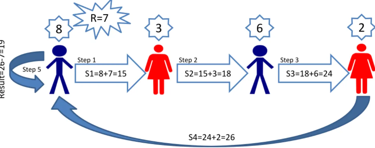
The initiator generates a random number R and adds it to her private number N1

to set a new number (S1 =N1+R) which is sent to the second party. Second party

adds her own private value toS1 (S2 =N2+S1) and sends it to the third party. This

procedure will be repeated until the sumSn is received by the initiator. The initiator

deducts the random number from Sn to calculate the actual sum value of the data

and broadcast it to the other parties. There are some security vulnerabilities on this

secure sum protocol. Two parties can compromise and reveal another party’s private

number (e.g. second and forth parties compromise to reveal third party’s private

number). Also, a malicious party can share an incorrect value, and as a result none

of the parties will receive the correct value except for the malicious party. These

is-Step 1 Step 2 Step 3 Step 5 S4=24+2=26 Step 4 Re su lt= 26-7= 19

8 R=7

3

6

2

S1=8+7=15 S2=15+3=18 S3=18+6=24

(33)

sues have been solved by other researchers such as Karr [34], though the new method

uses a centralized server, which is a bottleneck for the system. Chaum et al. [12]

proposed multiple secure protocols such as multiplication and enhanced by many

other researchers. As mentioned before, we mainly follow the proposed approaches

by Samet such as [52, 53, 50, 51] which includes various secure computation protocols

(34)

Chapter 4 Proposed Approach

To this chapter, we will discuss proposed approach to enhance security and privacy

in multi-party computation.

4.1 Data Distribution

Most of the time, data is distributed among different data custodians such as

hospi-tals. Because of security and privacy concerns, data custodians will not allow data

users (researchers) to execute a query on their databases directly. However, they are

willing to perform statistical methods without revealing their private information. As

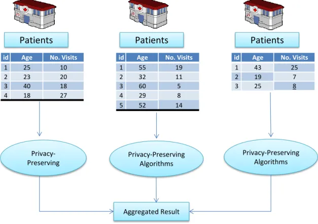
shown in Figure 3, data custodians are willing to collaborate using privacy-preserving

distributed algorithms to perform such methods. Therefore, secure computation is

needed for running a statistical method on all records. For example, each hospital

in St. John’s has a number of patients, and assume that a data user wants to run a

statistical method through all hospitals in St. John’s. It would be the same as a data

(35)

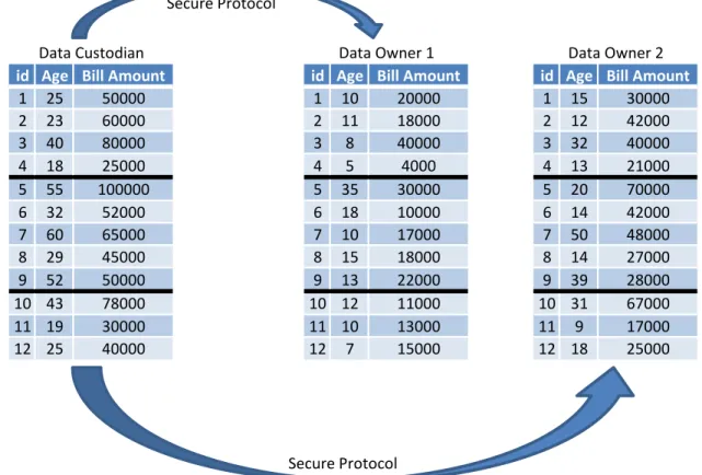
above distribution as Subset Data Distribution. The second type of distribution

id Age No. Visits id Age No. Visits id Age No. Visits

1 25 10 1 55 19 1 43 25

2 23 20 2 32 11 2 19 7

3 40 18 3 60 5 3 25 8

4 18 27 4 29 8

5 52 14

Patients

Privacy-Preserving Privacy-Preserving Algorithms Privacy-Preserving Algorithms Aggregated Result

Figure 3: subset data distribution

is a more complex process, and is used when the data custodians tend to store their

data in various data storages without revealing any information. As shown in Figure

4, each data value has been broken into n parts in a way that the summation of all

broken parts form the original data, where n is the number of data storages. For

example, imagine a data custodian wants to distribute the value of a specific column

such as Age of a specific patient whose age is 31 through three different data

(36)

distributes these values to data storages. It can be easily seen that the summation

of three values (10, 15 and 6) is equal to the original value (31). Data is distributed

between data storages in a way that none of them have any knowledge over the

orig-inal data. From this point, we refer to above distribution type as Partial Data

Distribution. In subset data distribution, data may be distributed through many hospitals and through various networks, which would result in loss of performance.

In partial data distribution, there is a chance of compromise between data storages

to reach the exact value of private information. There exists another type of data

id Age Bill Amount id Age Bill Amount id Age Bill Amount

1 25 50000 1 10 20000 1 15 30000 2 23 60000 2 11 18000 2 12 42000 3 40 80000 3 8 40000 3 32 40000 4 18 25000 4 5 4000 4 13 21000 5 55 100000 5 35 30000 5 20 70000 6 32 52000 6 18 10000 6 14 42000 7 60 65000 7 10 17000 7 50 48000 8 29 45000 8 15 18000 8 14 27000 9 52 50000 9 13 22000 9 39 28000 10 43 78000 10 12 11000 10 31 67000 11 19 30000 11 10 13000 11 9 17000 12 25 40000 12 7 15000 12 18 25000 Data Owner 2

Data Custodian Data Owner 1

Secure Protocol

(37)

distribution. Each party holds specific features of the data and they have the same

number of records and each row in their dataset represent the same record in all

parties with different features. As an example, we imagine the whole dataset is the

data custodian’s dataset in Figure 3. There are two parties. The first party, holds

only the first feature (e.g. Age) and the identifier’s column and the second party

holds the second feature (e.g. Bill Amount) and the identifier’s column of the data

custodian’s dataset. This data is distributed vertically which means that the whole

dataset is a union of all vertically partitioned datasets. In this thesis, this type of

data distribution is not covered and has not been implemented in the final web based

framework. The reader is encouraged to look into some of the works that have been

done on vertically partitioned data such as various works by Vaidya and Clifton or

Samet and Miri. Some of Clifton and Vaidya works include privacy-preserving

associ-ation rule mining [59], privacy-preserving k-means clustering [60], privacy-preserving

naive Bayes classifier [61] and privacy-preserving decision trees [62] over vertically

partitioned data. Some of Samet and Miri works include k-means clustering over

vertically and horizontally partitioned data [55] and secure comparison protocol in

the same paper, privacy-preserving back-propagation and extreme learning machine

algorithms over horizontally and vertically partitioned data [54] and two secure

pro-tocols for perceptron learning algorithm in neural networks [52] over horizontally and

(38)

4.2 Secure Building Blocks

For achieving secure computation, we use Paillier [46] cryptosystem, which is an

additive homomorphic encryption system. Paillier cryptosystems does not support

multiplicative homomorphism, thus the secure multiplication method proposed by

Samet and Miri [53] is used for secure computation. Suppose two parties P1, P2 want

to perform secure multiplication with their own private data (xP1 and xP2

respec-tively). P1 establishes a Paillier cryptosystem and shares her public key with P2. P1

encrypts her own private data and sends it to P2.

P1 :E(xP1)→P2 (4.1)

P2 generates a random private output yP2, encrypts the negative of yP2 (−yP2), and

multiplies it to the encrypted data sent by P1 to the power of her own private data

xP2 and sends the result to P1.

P2 :E(xP1)

xP₂ _∗_E(₋_y

P2)→P1 (4.2)

P1 decrypts the value given by P2, and sets it as her own private output yP1. It can

be easily shown that:

xP1 ∗xP2 =yP1 +yP2 (4.3)

Now, suppose the two parties want to perform a secure addition with their own private

data. P1 establishes a Paillier cryptosystem, and shares her public key with P2. P1

encrypts her own private data, and sends it to P2.

(39)

P2 generates a random private output yP2, and multiplies the encrypted data sent by

P1 to the encrypted value of her own private input and calculate the result to the

power of modular inverse of yP2 (y

−1

P2) and sends the result toP1.

P2 : (E(xP1)∗E(xP2))

y−_P1

2 →P₁ (4.5)

xP1 +xP2 =yP1 ∗yP2 (4.6)

Now, suppose the two parties want to perform a secure dot product [28] with their

own private data (we assume that both parties want to perform secure dot product

on their k number of records). P1 establishes a Paillier cryptosystem, and shares her

public key withP2. P1 encrypts all k records, and sends it toP2.

P1 :E(x1), E(x2),· · · , E(xk)→P2 (4.7)

P2 calculates the given encrypted record to the power of her own corresponding record

for each set of data and calculates the multiplication of all calculated records.

P2 :S =

k

Y

i=1

E(xi)yi _(4.8)

Afterwards, P2 generates a random private output yP2, and multiplies S to modular

inverse of yP2 and sends the result toP1.

P2 :S∗yP−21 →P1 (4.9)

k

Y

i=1

(40)

As shown below, we can extend secure multiplication for multiple parties when there

are more than two parties involved.

We assume we have x1∗x2 =y1+y2. Thus:

x1∗x2∗x3 = (y1+y2)∗x3 =y1x3+y2x3, (4.11)

We perform two secure two-party multiplications for y1x3 and y2x3.

y1∗x3 =z1+z31, y2∗x3 =z2+z32 => (4.12) x1∗x2∗x3 =z1+z31+z2+z32=z1+z2+z3 (4.13) We assume x1∗x2∗ · · · ∗xi =y1+y2+· · ·+yi. For (i+ 1): x1∗x2∗ · · · ∗xi∗xi+1 = (y1+y2+· · ·+yi)∗xi+1 = y1xi+1+y2xi+1+· · ·+yixi+1, (4.14)

We perform isecure two-party multiplications, so we have:

x1∗x2∗ · · · ∗xi∗xi+1 = z1+z(i+1)1+z2+z(i+1)2+· · ·+zi+z(i+1)i

= z1+z2+· · ·+zi+z(i+1) (4.15)

With a similar approach, we can extend the secure addition protocol for more than

two parties.

Now that we have our secure building blocks, we will show the protocols for

pop-ular statistical analysis methods. We assume that data user wants to perform any

statistical method between two parties for partial data distribution and subset data

distribution. As shown above, we can easily extend the methods to work on any

(41)

4.3 Statistical Analysis Methods

In this section, we will discuss the secure protocols for the computation of various

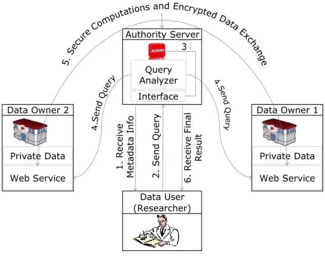
statistical analysis methods. As shown in Figure 5, the data user receives metadata

about data owners’ records. Then, she sends her preferred query to the data owners.

Data owners will perform required secure operations based on the query and each

of them will send the private output to the data user. By receiving those partial

information, the data user will be able to calculate the final result based on the given

data. Although, the mentioned process would be similar for both distribution types,

protocols for secure statistical analysis methods may differ. In this thesis, we will

discuss secure mean protocol as an example and the reader is referred to [51] for

further secure statistical methods analysis. In secure mean protocol, the data user

receives the metadata from data owners and sends the name of the attribute (e.g.

Age), which she wants to perform the secure mean protocol on to the first data owner

D1. Note that Age= (a1, a2,· · · , an) = (a1,1, a1,2,· · · , a1,n1, a2,1, a2,2,· · · , a2,n2), such

that ai,ni ∈Di and n=n1 +n2.

µ= n P i=1 ai n = n1 P i=1 a1,i+ n2 P i=1 a2,i n1+n2 (4.16)

After sending the query to the data owners, the process differs for subset or partial

data distributions. For subset data distribution, D1 establishes the encryption keys,

and sends the public keys to the second data owner D2. Then, D1 and D2 locally

calculate the summation of the corresponding column’s values such that:

Ai = ni X

j=1

(42)

Data Owner 2

Authority Server

Data Owner 1

Data User (Researcher)

Private Data Private Data

Web Service Interface 1 . Re cei ve Meta da ta I nfo 2 . Send Query Query Analyzer 3 6. Rec ei ve Fi na l Res ul t Web Service

Figure 5: Orocess Flow of the Protocol

Afterwards, data owners perform a secure addition for their private values A1 and

A2. Thus, each data owner has their own private output for the summation of their

values P O1D1 and P O1D2 where:

A1+A2 =P O1D1 ∗P O1D2 (4.18)

Each data owner has a number of records,n1andn2respectively. They perform secure

summation for their records, and as a result they will have another private output

P O2D1 andP O2D2 wheren1+n2 =P O2D1∗P O2D2. Each data owner will send their

(43)

the given data for each set of outputs (P O1D1 ∗P O1D2 and P O2D1 ∗P O2D2). By

doing so, data user has the summation of all values of the requested column and also

the summation of the records. By dividing these two values, the data user has the

final result such that:

µ= P O1D1 ∗P O1D2

P O2D1 ∗P O2D2

(4.19)

For partial data distribution, there is no need for the parties to perform secure

sum-mation for their number of records, i.e. they have the same number of records

(n1 = n2 = n). Thus, one of the parties sends the number of records to the data

user. The data user will multiply the given private outputs, and divide it by number

of records in order to get the final value of mean, such that:

µ= P O1D1 ∗P O1D2

n (4.20)

Other protocols include Secure Variance, Secure Skewness, Secure Correlation, and

Secure Chi-Square Test, which are proposed by Samet et al. [51]. In this thesis,

we implemented all these protocols in a web-based common framework and also we

extended the work by implementing more secure statistical methods such as student’s

t-test, linear regression and logistic regression for both data distribution types. The

proposed secure protocols for student’s t-test and linear regression for subset data

distribution and partial data distribution are completely original and also a new

approach has been proposed for secure logistic regression for partial data distribution.

4.3.1 Secure Student

t

-test

The t-test determines whether two sets of data are statistically different from each

(44)

for two-party computation. The t-test formula is as below:

t= _p µA−µB

varA/nA+varB/nB

(4.21)

where A and B are 2 sets of data, µA and µB are mean values of data sets A and B

respectively,varAandvarB are variance values of data setsA andB respectively and

nA and nB are the number of records of data sets A and B respectively. Thus, for

performing secure t-test protocol, two secure mean operations, two secure variance

operations and two secure count operations are needed for each one of the two sets of

data. The process is similar for partial data distribution and subset data distribution.

Note that the secure mean and secure variance protocols are different for partial

and subset data distribution. For calculating the mean and variance in partial data

distribution, there is no need for secure addition for computing the number of records,

because each party holds the same number of records as the original data owner. The

only difference is, both parties have portion of all values and and each value can be

computed by adding partial values.

4.3.2 Secure Linear Regression

Simple linear regression determines the relationship between two sets of data and is

used for assessing the association between two variables. Like other secure protocols,

(45)

linear regression formula is as below: y =a+bx (4.22) b= NΣXY −(ΣX)(ΣY) NΣX2₋_(ΣX)2 (4.23) a = ΣY −bΣX N (4.24)

wherexand yare the variables, bis the slope of the regression line, a is the intercept

point of the regression line and the y axis, N is the number of records, X is the first

variable and Y is the second variable.

For subset data distribution we know that:

N =n1+n2 (4.25)

where n1 is the number of records of the first party and n2 is the number of records

of the second party. Thus,

N X i=1 Xi = n1 X i=1 x1i+ n2 X i=1 x2i (4.26) N X i=1 Yi = n1 X i=1 y1i+ n2 X i=1 y2i (4.27) N X i=1 XiYi = n1 X i=1 x1iy1i+ n2 X i=1 x2iy2i (4.28) N X i=1 X_i2 = n1 X i=1 x2₁_i+ n2 X i=1 x2₂_i (4.29)

whereXi is thei-th record of first variable,Yi is thei-th record of second variable,x1i is the i-th record of first variable of first party, x2i is the i-th record of first variable of second party, y1i is the i-th record of second variable of first party and y2i is the

(46)

regression line (b), five secure additions are needed (N,ΣX,ΣY,ΣXY,ΣX2_).

For partial data distribution, the protocol is completely different. We know that in

partial data distribution, each party has the same number of records as the original

data and:

Xi =vi+ui (4.30)

Yi =wi+zi (4.31)

where vi is the i-th record of first variable of first party and ui is the i-th record of first variable of second party and the summation of corresponding values form the

original data. It is quite similar for Yi. Thus, N X 1 Xi = N X 1 (vi+ui) = N X 1 vi+ N X 1 ui (4.32) N X 1 Yi = N X 1 (wi+zi) = N X 1 wi+ N X 1 zi (4.33) N X 1 XiYi = N X 1 (vi+ui)(wi+zi) = N X 1 viwi+vizi+uiwi+uizi = N X 1 viwi+ N X 1 vizi+ N X 1 uiwi + N X 1 uizi (4.34) N X 1 X_i2 = N X 1 (vi+ui)2 = N X 1 v_i2+u2_i + 2viui = N X 1 v_i2+ N X 1 u2_i + 2 N X 1 viui (4.35)

(47)

For calculating 4.32 and 4.33, two secure additions are needed. In 4.34, PN

1 viwi

and PN

1 uizi can be computed locally, but two secure dot products are needed for

calculatingPN

1 viziand

PN

1 uiwi. Thus, three additional secure additions are needed

for the computation of 4.34. In 4.35, PN

1 v 2 i and PN 1 u 2

i can be computed locally,

but one secure dot product is needed for calculating PN

1 viui. Thus, two additional

secure additions are needed for the computation of 4.35. For calculating P

XP

Y,

one secure multiplication is needed. For computing NΣXY −(ΣX)(ΣY), another

secure addition is needed. Also, for calculating NΣX2 −(ΣX)2 another additional

secure addition is needed. In total, for calculating the slope of the regression line (b)

in partial data distribution, three secure dot products, one secure multiplication and

nine secure additions are needed.

4.3.3 Secure Logistic Regression

Logistic regression is a regression model that determines the relationship between one

or more independent variable(s) with a dependent variable which is categorical. It is

used to estimate the probability of a dependent variable based on independent

vari-able(s). Like other statistical analysis methods, logistic regression should be broken in

a way that each party calculates the private output for themselves and the final result

can be calculated using private output(s) for two party computation. To estimate the

parameters that best fit the data, maximum likelihood estimation is utilized. Our

model is based on the work done by Samet [50]. We denote the number of

indepen-dent samples by M in our dataset and a random dependent variable by Z which has

(48)

have N different combinations. We denote the samples with combination i by ni.

We denote a column vector with i elements which stores the number of records for

Z where the value is 1 byyi. The probability of Z being 1 for the i-th element has

been shown by πi. The independent variables could be shown in a matrix X which

has the same number of rows as our sample dataset (M) andK+1 columns where K

is the number of independent variables. Every element’s value of the first column of

the matrix is 1. For each independent variable, we should compute a vector β with

K+1 and an intercept. Newton-Raphson method has been used for this purpose. β

can ba computed as below:

βz =βz−1+ [XTW X]−1XT(y−µ) (4.36)

µi =niπi,

πi =P(Zi = 1|i),

whereβ0 is an initial approximation which can be based on the previous experiments

on a similar dataset or it can be generated randomly and W is a diagonal N ∗N

matrix. In matrixW, all the elements except for elements on its diagonal (ei) have a

zero value, where ei can be computed as below:

ei =niπi(1−πi)

We consider a specific threshold and the above computation will iterate until the

(49)

computation ofµi and wi,i is as below: µi = eXi∗Bz 1 +eXi∗Bz (4.37) wi,i = eXi∗Bz (1 +eXi∗Bz₎2 (4.38)

The X, W and µmatrices are as below:

X =           1 x11 x12 . . . x1K 1 x21 x22 . . . x2K . . . . 1 xN1 xN2 . . . xN K           W =           n1π1(1−π1) 0 0 . . . 0 0 n2π2(1−π2) 0 . . . 0 . . . . 0 0 0 . . . nNπN(1−πN)           µ=           n1π1 n2π2 . . . . nNπN          

For subset data distribution, each party has a subset of the whole data. We assume

that the first party has j1 number of records and the second party has j2 number of

records. Thus:

(50)

The first party’s X and µmatrices are as below: X1 =           1 x11 x12 . . . x1K 1 x21 x22 . . . x2K . . . . 1 xj11 xj12 . . . xj1K           µ1 =           n1π1 n2π2 . . . . nj1πj1          

The second party’s matrices are as below:

X2 =           1 x(j1+1)1 x(j1+1)2 . . . x(j1+1)K 1 x(j1+2)1 x(j1+2)2 . . . x(j1+2)K . . . . 1 xN1 xN2 . . . xN K           µ2 =           nj1+1πj1+1 nj1+2πj1+2 . . . . nNπN          

The W matrix is public. For calculating 4.36, we proceed as follow:

XTW=          1 1 . . . 1 1 . . .1 x11 x21 . . . xj1 1 x(j1 +1)1 . . . xN1 . . . . x1K xx2K . . . xj1K x(j_{1 +1)}K xN K                   n1π1(1−π1) . . . 0 0 . . . 0 . . . . 0 . . . nNπN(1−πN)          XTW=          n1π1(1−π1) n2π2(1−π2) . . . nNπN(1−πN) x11n1π1(1−π1) x21n2π2(1−π2) . . . xN1nNπN(1−πN) . . . . x1Kn1π1(1−π1) x2Kn1π1(1−π1) . . . xN KnNπN(1−πN)         

(51)

XTW X=                 n1π1(1−π1) . . . nNπN(1−πN) . . . . xj1 1nj1πj1(1−πj1) . . . xN1nNπN(1−πN) x(j1 +1)1nj1 +1πj1 +1(1−πj1 +1) . . . xN1nNπN(1−πN) . . . . x1Kn1π1(1−π1) . . . xN KnNπN(1−πN)                                 1 . . . x1K . . . . 1 . . . xj1K 1 . . . x(j1 +1)K . . . . 1 . . . xN K                 =                 n1π1(1−π1) +· · ·+nNπN(1−πN) . . . n1π1(1−π1)x1K+· · ·+nNπN(1−πN)xN K . . . . xj1 1nj1πj1(1−πj1) +· · ·+xN1nNπN(1−πN) . . . xj1 1nj1πj1(1−πj1)x1K+· · ·+xN1nNπN(1−πN)xN K x(j_{1 +1)1}nj1 +1πj1 +1(1−πj1 +1) +· · ·+xN1nNπN(1−πN) . . . x(j_{1 +1)1}nj1 +1πj1 +1(1−πj1 +1)x1K+· · ·+xN1nNπN(1−πN)xN K . . . . x₁_Kn1π1(1−π1) +· · ·+xN KnNπN(1−πN) . . . x1Kn1π1(1−π1)x1K+· · ·+xN KnNπN(1−πN)x1KxN K                

The firstj1 summation in each cell can be done by the first party and the second party

can calculate the rest. Thus, the above matrix can be broken into the summation of

two matrices which can be calculated by each party separately, such that:

XTW X =M1+M2 (4.39)

whereM1 and M2 are the corresponding matrices of the first party and second party

respectively. In order to fully compute 4.36, we should be able to securely compute

the inverse of a matrix. For computing the inverse of a matrix, we use a method

proposed by Han et al. [31] in which two parties can compute their private shares as

below:

[M1+M2]−1 =V1+V2 (4.40)

Thus, to calculate [XTW X]−1, one secure matrix inverse computation is needed. For

calculating XT(y−µ), two secure matrix multiplications (XTy and XTµ) and one

secure addition (XTy−XTµ) are needed. Secure multiplication of matrices for partial data distribution has been shown in [50] such that:

(52)

Where P and Q are the two matrices of the first party and the second party respec-tively. Thus, we have:

XTy−XTµ=W1+W2 (4.42)

[XTW X]−1 =V1+V2 (4.43)

=>[XTW X]−1XT(y−µ) = (V1+V2)(W1+W2) =V1W1+V1W2+V2W1+V2W2

(4.44)

V1W1 and V2W2 can be computed locally by the first party and the second party

respectively. Moreover, V1W2 and V2W1 can be computed using secure matrix

mul-tiplication. For more in-depth details, reader is encouraged to read the original

pa-per [50].

For partial data distribution, each party hasN rows of records, but the original value can be formed by the summation of all broken values as mentioned before. In order

to fully compute 4.36, we should be able to securely compute the inverse of a

ma-trix. Thus, to calculate [XTW X]−1 in partial data distribution, two secure matrix multiplications and one secure matrix inverse computation is needed. For calculating

XT(y−µ), two secure matrix multiplications (XTyandXTµ) and one secure addition (XTy−XTµ) are needed.

4.4 Complexity Assumptions

As mentioned before, the proposed secure computation framework is based on Paillier

Cryptosystem [46]. The security relies on the security of discrete logarithms which

are known to be hard to solve. There is no efficient algorithm to solve the worst case

(53)

complexity is quite the same as the worst case scenario. With major improvement

and usage of cloud computing and powerful computer systems, 2048-bit key is

rec-ommended for using in cryptosystems.

4.4.1 Building Blocks Complexity

Complexity analysis of all secure building blocks have been shown below. We assume

that the Paillier cryptosystem has been established by one of the data owners. The

public key exchange stage between parties through authority server has not been

considered in the communication cost, because it will only be executed once for every

protocol. The calculation of computation costs for various building blocks are based

on previous works, but the calculation of communication costs is done by the author

because the communication costs are dependent on the proposed system.

4.4.1.1 Secure Multiplication

There are two encryptions and one decryption in two-party secure multiplication. By

assuming that the cost of encryption and decryption are equal, we have:

Computation cost = 3a

where a is the cost of encryption and decryption.

Data owners are not connected together directly in the proposed system; however,

they are able to exchange data through authority server. For two-party secure

(54)

Thus:

Communication cost = 4b

where b is the number of bits exchanged for each message.

To improve the performance of multi-party secure multiplicationof n data owners,

data owners could be divided into two groups, i.e. P1, P2,· · · , Pbn

2candPb

n

2c+1,· · · , Pn

are considered the first group and the second group. By recursively dividing the new

groups each time until all groups are a pair of two parties, the overall time would

improve significantly. So, by doing above, there are n(n₂+1) encryptions and n(n₂−1) decryptions for this building block. Thus:

Computation cost = (n(n+ 1)

2 +

n(n−1)

2 )a=n

2_a

We saw that in the two-party secure multiplication the cost is 4b. By denoting this

cost for n parties as C(n) wheren ≥3, we have:

Communication cost =C(n) = C(bn 2c) +C(d n 2e) + (b n 2c ∗(d n 2e+ 1))b (4.45) 4.4.1.2 Secure Addition

There are two encryptions and one decryption in two-party secure multiplication. By

assuming that the cost of encryption and decryption are equal, we have:

Computation cost = 3a

For two-party secure addition, four messages are exchanged between data owners and

authority server. Thus:

(55)

where b is the number of bits exchanged for each message.

There are (n−1)(₂n+2) encryptions and n(n₂−1) decryptions for n party secure addition. Thus:

Computation cost = ((n−1)(n+ 2)

2 +

n(n−1)

2 )a = (n−1)(n+ 1)a

All messages are sent from data owners to authority server and then from authority

server to other data owners. Therefore,

Communication cost = (n−1)(n+ 2)b (4.46)

4.4.1.3 Secure Dot Product

If the secure dot product performed on krecords, there are k+ 1 encryptions and one

decryption in two-party secure dot product. By assuming that the cost of encryption

and decryption are equal, we have:

Computation cost = (k+ 2)a

For two-party secure dot product, four messages are exchanged between data owners

and authority server. Thus:

Communication cost = 4b

Privacy-preserving statistical analysis methods and their applications on health research