MODEL EVALUATION GUIDELINES FOR SYSTEMATIC QUANTIFICATION OF ACCURACY IN WATERSHED SIMULATIONS

M

ODEL

E

VALUATION

G

UIDELINES

FOR

S

YSTEMATIC

Q

UANTIFICATION

OF

A

CCURACY

IN

W

ATERSHED

S

IMULATIONS

D. N. Moriasi, J. G. Arnold, M. W. Van Liew, R. L. Bingner, R. D. Harmel, T. L. Veith

ABSTRACT. Watershed models are powerful tools for simulating the effect of watershed processes and management on soil and

water resources. However, no comprehensive guidance is available to facilitate model evaluation in terms of the accuracy of simulated data compared to measured flow and constituent values. Thus, the objectives of this research were to: (1) determine recommended model evaluation techniques (statistical and graphical), (2) review reported ranges of values and corresponding performance ratings for the recommended statistics, and (3) establish guidelines for model evaluation based on the review results and project-specific considerations; all of these objectives focus on simulation of streamflow and transport of sediment and nutrients. These objectives were achieved with a thorough review of relevant literature on model application and recommended model evaluation methods. Based on this analysis, we recommend that three quantitative statistics, Nash-Sutcliffe efficiency (NSE), percent bias (PBIAS), and ratio of the root mean square error to the standard deviation of measured data (RSR), in addition to the graphical techniques, be used in model evaluation. The following model evaluation performance ratings were established for each recommended statistic. In general, model simulation can be judged as satisfactory if NSE > 0.50 and RSR < 0.70, and if PBIAS + 25% for streamflow, PBIAS + 55% for sediment, and PBIAS

+ 70% for N and P. For PBIAS, constituent-specific performance ratings were determined based on uncertainty of measured data. Additional considerations related to model evaluation guidelines are also discussed. These considerations include: single-event simulation, quality and quantity of measured data, model calibration procedure, evaluation time step, and project scope and magnitude. A case study illustrating the application of the model evaluation guidelines is also provided.

Keywords. Accuracy, Model calibration and validation, Simulation, Watershed model.

omputer-based watershed models can save time and money because of their ability to perform long-term simulation of the effects of watershed pro-cesses and management activities on water quality, water quantity, and soil quality. These models also facilitate the simulation of various conservation program effects and aid policy design to mitigate water and soil quality degrada-tion by determining suitable conservadegrada-tion programs for par-ticular watersheds and agronomic settings. In order to use model outputs for tasks ranging from regulation to research, models should be scientifically sound, robust, and defensible (U.S. EPA, 2002).

Submitted for review in May 2006 as manuscript number SW 6494; ap-proved for publication by the Soil & Water Division of ASABE in March 2007.

The authors are Daniel N. Moriasi, ASABE Member Engineer, Hydrologist, USDA-ARS Grazinglands Research Laboratory, El Reno, Oklahoma; Jeffrey G. Arnold, Supervisory Agricultural Engineer, USDA-ARS Grassland Soil and Water Research Laboratory, Temple, Texas; Mi-chael W. Van Liew, ASABE Member Engineer, Environmental Science Specialist, Water Quality Planning Bureau, Montana Department of Envi-ronmental Quality, Helena, Montana; Ronald L. Bingner, ASABE Mem-ber Engineer, Agricultural Engineer, USDA-ARS Watershed Physical Pro-cesses Research Unit, Oxford, Mississippi; R. Daren Harmel, ASABE Member Engineer, Agricultural Engineer, USDA-ARS Grassland Soil and Water Research Laboratory, Temple, Texas; and Tamie L. Veith, ASABE Member Engineer, Agricultural Engineer, USDA-ARS Pasture Systems and Watershed Management Research Unit, University Park, Pennsylva-nia. Corresponding author: Daniel N. Moriasi, USDA-ARS Grazinglands Research Laboratory, 7207 W. Cheyenne St., El Reno, OK 73036-0000; phone: 405-262-5291, ext. 263; fax: 405-262-0133; e-mail: [email protected].

Sensitivity analysis is the process of determining the rate of change in model output with respect to changes in model inputs (parameters). It is a necessary process to identify key parameters and parameter precision required for calibration (Ma et al., 2000). Model calibration is the process of estimat-ing model parameters by comparestimat-ing model predictions (out-put) for a given set of assumed conditions with observed data for the same conditions. Model validation involves running a model using input parameters measured or determined dur-ing the calibration process. Accorddur-ing to Refsgaard (1997), model validation is the process of demonstrating that a given site-specific model is capable of making “sufficiently accu-rate” simulations, although “sufficiently accuaccu-rate” can vary based on project goals. According to the U.S. EPA (2002), the process used to accept, reject, or qualify model results should be established and documented before beginning model eval-uation. Although ASCE (1993) emphasized the need to clear-ly define model evaluation criteria, no commonclear-ly accepted guidance has been established, but specific statistics and per-formance ratings for their use have been developed and used for model evaluation (Donigian et al., 1983; Ramanarayanan et al., 1997; Gupta et al., 1999; Motovilov et al., 1999; Saleh et al., 2000; Santhi et al., 2001; Singh et al., 2004; Bracmort et al., 2006; Van Liew et al., 2007). However, these perfor-mance ratings are model and project specific. Standardized guidelines are needed to establish a common system for judg-ing model performance and comparjudg-ing various models (ASCE, 1993). Once established, these guidelines will assist modelers in preparing and reviewing quality assurance proj-ect plans for modeling (U.S. EPA, 2002) and will increase ac-countability and public acceptance of models to support

scientific research and to guide policy, regulatory, and man-agement decision-making.

A number of publications have addressed model evalua-tion statistics (Willmott, 1981; ASCE, 1993; Legates and McCabe, 1999), but they do not include recently developed statistics (e.g., Wang and Melesse, 2005; Parker et al., 2006). More importantly, none of the previous publications provide guidance on acceptable ranges of values for each statistic. Borah and Bera (2004) present an excellent review of values for various statistics used in hydrologic and nonpoint-source model applications, but more elaborate analysis is needed to aid modelers in determining performance ratings for these statistics.

In most watershed modeling projects, model output is compared to corresponding measured data with the assump-tion that all error variance is contained within the predicted values and that observed values are error free. In discussions of model evaluation statistics, Willmott (1981) and ASCE (1993) do recognize that measured data are not error free, but measurement error is not considered in their recommenda-tions perhaps because of the relative lack of data on measure-ment uncertainty. However, uncertainty estimates for measured streamflow and water quality data have recently become available (Harmel et al., 2006) and should be consid-ered when calibrating, validating, and evaluating watershed models because of differences in inherent uncertainty be-tween measured flow, sediment, and nutrient data.

The importance of standardized guidelines for model evaluation is illustrated by the Conservation Effects Assess-ment Project Watershed AssessAssess-ment Study (CEAP-WAS, 2005). The CEAP-WAS seeks to quantify the environmental benefits of conservation practices supported by USDA in the 2002 Farm Bill, also known as the Farm Security and Rural Investment Act. One of the CEAP-WAS goals is to formulate guidelines for calibration, validation, and application of models used in CEAP to simulate environmental effects of conservation practices. Thus, based on the need for standard-ized model evaluation guidelines to support watershed mod-eling in CEAP-WAS and other projects, the objectives for the present research were to: (1) determine recommended model evaluation techniques (statistical and graphical), (2) review reported ranges of values and corresponding performance ratings for the recommended statistics, and (3) establish guidelines for model evaluation based on the review results and project-specific considerations. In addition, a case study illustrating the application of the model evaluation guide-lines was provided. This research focuses on watershed mod-el evaluation guidmod-elines for streamflow, sediments, and nutrients. Throughout this article, “model evaluation” refers to the applicable steps of sensitivity analysis, calibration, val-idation, uncertainty analysis, and application.

M

MODEL EVALUATION TECHNIQUES

To determine recommended techniques for watershed model evaluation, an extensive review was conducted on published literature related to calibration, validation, and ap-plication of watershed models. Specifically, the information compiled focused on the strengths and weaknesses of each statistical and graphical technique and on recommendations for their application. The recommended model evaluation

statistics were selected based on the following factors: (1) ro-bustness in terms of applicability to various constituents, models, and climatic conditions; (2) commonly used, accept-ed, and recommended in published literature; and (3) identi-fied strengths in model evaluation. The trade-off between long-term bias and residual variance was also considered, as recommended by Boyle et al. (2000). Bias measures the aver-age tendency of the simulated constituent values to be larger or smaller than the measured data. Residual variance is the difference between the measured and simulated values, often estimated by the residual mean square or root mean square er-ror (RMSE). According to Boyle et al. (2000), optimizing RMSE during model calibration may give small error vari-ance but at the expense of significant model bias. The com-pilation of recommended statistics was also constrained by the recommendation of Legates and McCabe (1999) to in-clude at least one dimensionless statistic and one absolute er-ror index statistic with additional information such as the standard deviation of measured data, and to include at least one graphical technique as well.

REPORTED VALUE RANGESAND PERFORMANCE RATINGS FOR RECOMMENDED STATISTICS

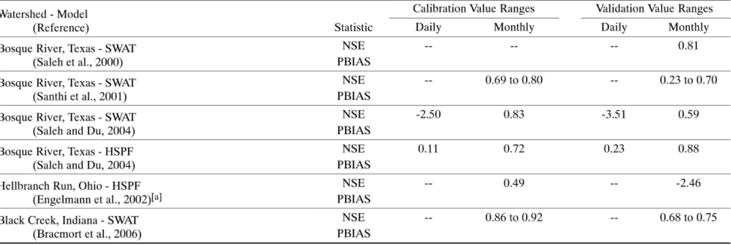
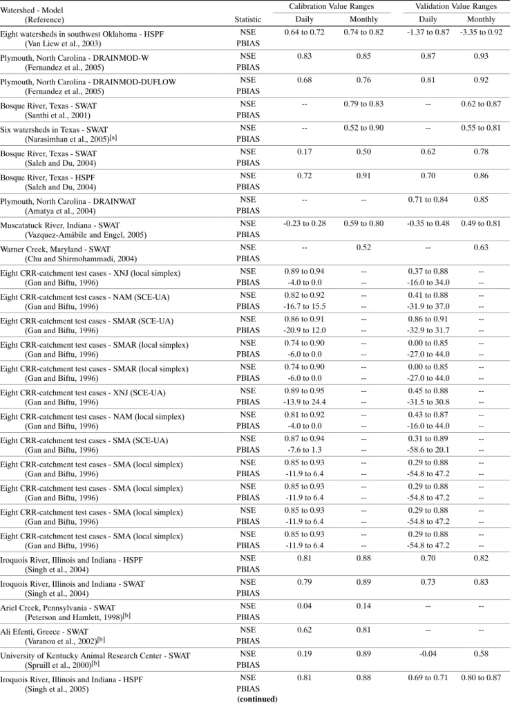
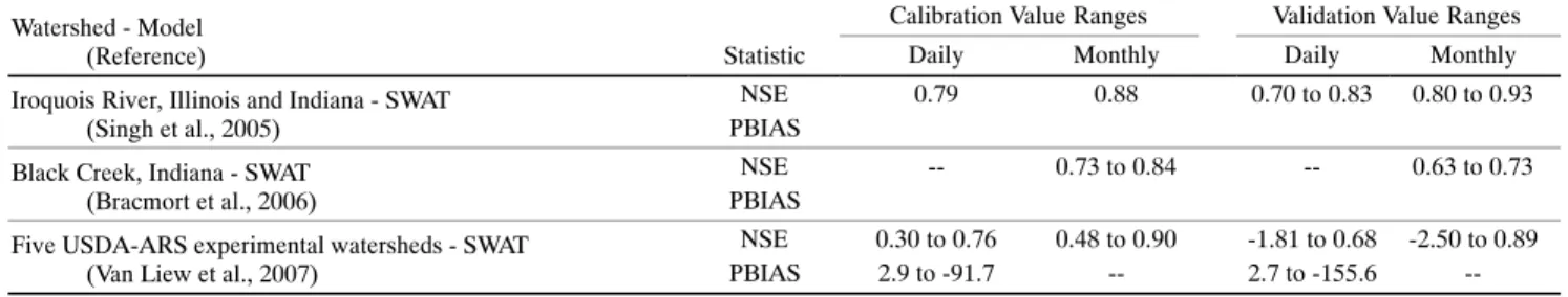
Additional literature review was conducted to determine published ranges of values and performance ratings for rec-ommended model evaluation statistics. Reported daily and monthly values during the calibration and validation periods for streamflow, sediment, and nutrients are recorded along with the model used for evaluation in tables A-1 through A-9 in the Appendix. All the reported data were analyzed and compiled into a summary of daily and monthly value ranges for different constituents during calibration and validation (table 1). The summary values in table 1 include the sample size of the reported values (n) and the minimum, maximum, and median of the values reported for streamflow, surface runoff, sediment, organic, mineral and total nitrogen, and or-ganic, mineral, and total phosphorus.

MODEL EVALUATION GUIDELINES

General model evaluation guidelines that consider the rec-ommended model evaluation statistics with corresponding performance ratings and appropriate graphical analyses were then established. A calibration procedure chart for flow, sedi-ment, and nutrients, similar to the one proposed by Santhi et al. (2001), is included to assist in application of the model evaluation guidelines to manual model calibration. It is noted, however, that these guidelines should be adjusted by the modeler based on additional considerations such as: single-event simulation, quality and quantity of measured data, model calibration procedure, evaluation time step, and project scope and magnitude. Additionally, a brief discussion of the implications of unmet performance ratings is provided.

R

D

Both statistical and graphical model evaluation tech-niques were reviewed. The quantitative statistics were divid-ed into three major categories: standard regression, dimensionless, and error index. Standard regression statistics determine the strength of the linear relationship between sim-ulated and measured data. Dimensionless techniques provide

a relative model evaluation assessment, and error indices quantify the deviation in the units of the data of interest (Leg-ates and McCabe, 1999). A brief discussion of numerous model evaluation statistics (both recommended statistics and statistics not selected for recommendation) appears subse-quently; however, the relevant calculations are provided only for the recommended statistics.

Several graphical techniques are also described briefly be-cause graphical techniques provide a visual comparison of simulated and measured constituent data and a first overview of model performance (ASCE, 1993) and are essential to ap-propriate model evaluation (Legates and McCabe, 1999). Based on recommendations by ASCE (1993) and Legates and McCabe (1999), we recommend that both graphical tech-niques and quantitative statistics be used in model evalua-tion.

MODEL EVALUATION STATISTICS (STANDARD REGRESSION)

Slope and y-intercept: The slope and y-intercept of the best-fit regression line can indicate how well simulated data match measured data. The slope indicates the relative rela-tionship between simulated and measured values. The y-intercept indicates the presence of a lag or lead between model predictions and measured data, or that the data sets are not perfectly aligned. A slope of 1 and y-intercept of 0 indi-cate that the model perfectly reproduces the magnitudes of measured data (Willmott, 1981). The slope and y-intercept are commonly examined under the assumption that measured and simulated values are linearly related, which implies that all of the error variance is contained in simulated values and that measured data are error free (Willmott, 1981). In reality, measured data are rarely, if ever, error free. Harmel et al. (2006) showed that substantial uncertainty in reported water quality data can result when individual errors from all proce-dural data collection categories are considered. Therefore, care needs to be taken while using regression statistics for model evaluation.

Pearson’s correlation coefficient (r) and coefficient of determination (R2_{): Pearson’s correlation coefficient (r)}

and coefficient of determination (R2_{) describe the degree of}

collinearity between simulated and measured data. The cor-relation coefficient, which ranges from −1 to 1, is an index of the degree of linear relationship between observed and simu-lated data. If r = 0, no linear relationship exists. If r = 1 or −1, a perfect positive or negative linear relationship exists. Simi-larly, R2 _{describes the proportion of the variance in measured}

data explained by the model. R2 _{ranges from 0 to 1, with}

high-er values indicating less high-error variance, and typically values greater than 0.5 are considered acceptable (Santhi et al., 2001, Van Liew et al., 2003). Although r and R2 _{have been}

widely used for model evaluation, these statistics are over-sensitive to high extreme values (outliers) and inover-sensitive to additive and proportional differences between model predic-tions and measured data (Legates and McCabe, 1999). MODEL EVALUATION STATISTICS (DIMENSIONLESS)

Index of agreement (d): The index of agreement (d) was developed by Willmott (1981) as a standardized measure of the degree of model prediction error and varies between 0 and 1. A computed value of 1 indicates a perfect agreement be-tween the measured and predicted values, and 0 indicates no agreement at all (Willmott, 1981). The index of agreement

represents the ratio between the mean square error and the “potential error” (Willmott, 1984). The author defined poten-tial error as the sum of the squared absolute values of the dis-tances from the predicted values to the mean observed value and distances from the observed values to the mean observed value. The index of agreement can detect additive and pro-portional differences in the observed and simulated means and variances; however, d is overly sensitive to extreme val-ues due to the squared differences (Legates and McCabe, 1999). Legates and McCabe (1999) suggested a modified in-dex of agreement (d1) that is less sensitive to high extreme values because errors and differences are given appropriate weighting by using the absolute value of the difference instead of using the squared differences. Although d1 has been proposed as an improved statistic, its limited use in the literature has not provided extensive information on value ranges.

Nash-Sutcliffe efficiency (NSE): The Nash-Sutcliffe ef-ficiency (NSE) is a normalized statistic that determines the relative magnitude of the residual variance (“noise”) compared to the measured data variance (“information”) (Nash and Sutcliffe, 1970). NSE indicates how well the plot of observed versus simulated data fits the 1:1 line. NSE is computed as shown in equation 1:

(

)

(

)

∑

∑

where Yi obs is the ith observation for the constituent being

evaluated, Yisim is the ith simulated value for the constituent

being evaluated, Ymean _{is the mean of observed data for the}

constituent being evaluated, and n is the total number of ob-servations.

NSE ranges between −∞ and 1.0 (1 inclusive), with NSE = 1 being the optimal value. Values between 0.0 and 1.0 are generally viewed as acceptable levels of performance, whereas values <0.0 indicates that the mean observed value is a better predictor than the simulated value, which indicates unacceptable performance.

NSE was recommended for two major reasons: (1) it is recommended for use by ASCE (1993) and Legates and McCabe (1999), and (2) it is very commonly used, which pro-vides extensive information on reported values. Sevat and Dezetter (1991) also found NSE to be the best objective func-tion for reflecting the overall fit of a hydrograph. Legates and McCabe (1999) suggested a modified NSE that is less sensi-tive to high extreme values due to the squared differences, but that modified version was not selected because of its limited use and resulting relative lack of reported values.

Persistence model efficiency (PME): Persistence model efficiency (PME) is a normalized model evaluation statistic that quantifies the relative magnitude of the residual variance (“noise”) to the variance of the errors obtained by the use of a simple persistence model (Gupta et al., 1999). PME ranges from 0 to 1, with PME = 1 being the optimal value. PME val-ues should be larger than 0.0 to indicate “minimally accept-able” model performance (Gupta et al., 1999). The power of PME is derived from its comparison of model performance with a simple persistence forecast model. According to Gupta et al. (1999), PME is capable of clearly indicating poor model

performance, but it has been used only occasionally in the lit-erature, so a range of reported values is not available.

Prediction efficiency (Pe): Prediction efficiency (Pe), as

explained by Santhi et al. (2001), is the coefficient of deter-mination (R2_{) calculated by regressing the rank (descending)}

of observed versus simulated constituent values for a given time step. Pe determines how well the probability

distribu-tions of simulated and observed data fit each other. However, it has not been used frequently enough to provide extensive information on ranges of values. In addition, it may not ac-count for seasonal bias.

Performance virtue statistic (PVk): The performance

virtue statistic (PVk) is the weighted average of the

Nash-Sutcliffe coefficients, deviations of volume, and error func-tions across all flow gauging stafunc-tions within the watershed of interest (Wang and Melesse, 2005). PVk was developed to

as-sess if watershed models can satisfactorily predict all aspects (profile, volume, and peak) of observed flow hydrographs for watersheds with more than one gauging station (Wang and Melesse, 2005). PVk can range from −∞ to 1.0, with a PVk

value of 1.0 indicating that the model exactly simulates all three aspects of observed flow for all gauging stations within the watershed. A negative PVk value indicates that the

aver-age of observed streamflow values is better than simulated streamflows (Wang and Melesse, 2005). PVk was developed

for use in snow-fed watersheds; therefore, it may be neces-sary to make adjustments to this statistic for rain-fed wa-tersheds. PVk was not selected for recommendation because

it was developed for streamflow only. In addition, PVk was

only recently developed; thus, extensive information on val-ue ranges is not available.

Logarithmic transformation variable (e): The logarith-mic transformation variable (e) is the logarithm of the pre-dicted/observed data ratio (E) that was developed to address the sensitivity of the watershed-scale pesticide model error index (E) to the estimated pesticide application rates (Parker et al., 2006). The value of e is centered on zero, is symmetri-cal in under- or overprediction, and is approximately normal-ly distributed (Parker et al., 2006). If the simulated and measured data are in complete agreement, then e = 0 and E = 1.0. Values of e < 0 are indicative of underprediction; values > 0 are indicative of overprediction. Although e has great po-tential as an improved statistical technique for assessing model accuracy, it was not selected because of its recent de-velopment and limited testing and application.

MODEL EVALUATION STATISTICS (ERROR INDEX)

MAE, MSE, and RMSE: Several error indices are com-monly used in model evaluation. These include mean abso-lute error (MAE), mean square error (MSE), and root mean square error (RMSE). These indices are valuable because they indicate error in the units (or squared units) of the con-stituent of interest, which aids in analysis of the results. RMSE, MAE, and MSE values of 0 indicate a perfect fit. Singh et al. (2004) state that RMSE and MAE values less than half the standard deviation of the measured data may be con-sidered low and that either is appropriate for model evalua-tion. A standardized version of the RMSE was selected for recommendation and is described later in this section.

Percent bias (PBIAS): Percent bias (PBIAS) measures the average tendency of the simulated data to be larger or smaller than their observed counterparts (Gupta et al., 1999).

The optimal value of PBIAS is 0.0, with low-magnitude val-ues indicating accurate model simulation. Positive valval-ues in-dicate model underestimation bias, and negative values indicate model overestimation bias (Gupta et al., 1999). PBIAS is calculated with equation 2:

(

)

( )

∑

∑

where PBIAS is the deviation of data being evaluated, ex-pressed as a percentage.

Percent streamflow volume error (PVE; Singh et al., 2004), prediction error (PE; Fernandez et al., 2005), and per-cent deviation of streamflow volume (Dv) are calculated in

a similar manner as PBIAS. The deviation term (Dv) is used

to evaluate the accumulation of differences in streamflow volume between simulated and measured data for a particular period of analysis.

PBIAS was selected for recommendation for several rea-sons: (1) Dv was recommended by ASCE (1993), (2) Dv is

commonly used to quantify water balance errors and its use can easily be extended to load errors, and (3) PBIAS has the ability to clearly indicate poor model performance (Gupta et al., 1999). PBIAS values for streamflow tend to vary more, among different autocalibration methods, during dry years than during wet years (Gupta et al., 1999). This fact should be considered when attempting to do a split-sample evalua-tion, one for calibration and one for validation.

RMSE-observations standard deviation ratio (RSR): RMSE is one of the commonly used error index statistics (Chu and Shirmohammadi, 2004; Singh et al., 2004; Vasquez-Amábile and Engel, 2005). Although it is common-ly accepted that the lower the RMSE the better the model per-formance, only Singh et al. (2004) have published a guideline to qualify what is considered a low RMSE based on the ob-servations standard deviation. Based on the recommendation by Singh et al. (2004), a model evaluation statistic, named the RMSE-observations standard deviation ratio (RSR), was de-veloped. RSR standardizes RMSE using the observations standard deviation, and it combines both an error index and the additional information recommended by Legates and McCabe (1999). RSR is calculated as the ratio of the RMSE and standard deviation of measured data, as shown in equa-tion 3:

(

)

(

)

∑

∑

RSR incorporates the benefits of error index statistics and includes a scaling/normalization factor, so that the resulting statistic and reported values can apply to various constitu-ents. RSR varies from the optimal value of 0, which indicates zero RMSE or residual variation and therefore perfect model simulation, to a large positive value. The lower RSR, the low-er the RMSE, and the bettlow-er the model simulation plow-erfor- perfor-mance.

Daily root-mean square (DRMS): The daily root-mean square (DRMS), which is a specific application of the RMSE, computes the standard deviation of the model prediction er-ror (difference between measured and simulated values). The smaller the DRMS value, the better the model performance (Gupta et al., 1999). Gupta et al. (1999) determined that DRMS increased with wetness of the year, indicating that the forecast error variance is larger for higher flows. According to Gupta et al. (1999), DRMS had limited ability to clearly indicate poor model performance.

GRAPHICAL TECHNIQUES

Graphical techniques provide a visual comparison of sim-ulated and measured constituent data and a first overview of model performance (ASCE, 1993). According to Legates and McCabe (1999), graphical techniques are essential to ap-propriate model evaluation. Two commonly used graphical

techniques, hydrographs and percent exceedance probability curves, are especially valuable. Other graphical techniques, such as bar graphs and box plots, can also be used to examine seasonal variations and data distributions.

A hydrograph is a time series plot of predicted and mea-sured flow throughout the calibration and validation periods. Hydrographs help identify model bias (ASCE, 1993) and can identify differences in timing and magnitude of peak flows and the shape of recession curves.

Percent exceedance probability curves, which often are daily flow duration curves, can illustrate how well the model reproduces the frequency of measured daily flows throughout the calibration and validation periods (Van Liew et al., 2007). General agreement between observed and simulated fre-quencies for the desired constituent indicates adequate simu-lation over the range of the conditions examined (Singh et al., 2004).

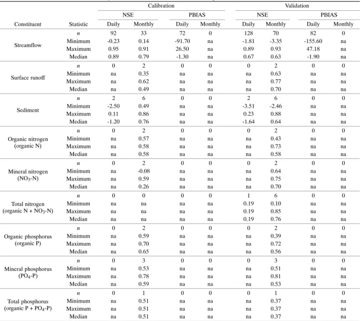
Table 1. Summary statistics from the literature review of reported NSE and PBIAS values.[a]

Calibration Validation

NSE PBIAS NSE PBIAS

Constituent Statistic Daily Monthly Daily Monthly Daily Monthly Daily Monthly

Streamflow n 92 33 72 0 128 70 82 0 Minimum -0.23 0.14 -91.70 na -1.81 -3.35 -155.60 na Maximum 0.95 0.91 26.50 na 0.89 0.93 47.18 na Median 0.89 0.79 -1.30 na 0.67 0.63 -1.90 na Surface runoff n 0 2 0 0 0 2 0 0 Minimum na 0.35 na na na 0.63 na na Maximum na 0.62 na na na 0.77 na na Median na 0.49 na na na 0.70 na na Sediment n 2 6 0 0 2 6 0 0 Minimum -2.50 0.49 na na -3.51 -2.46 na na Maximum 0.11 0.86 na na 0.23 0.88 na na Median -1.20 0.76 na na -1.64 0.64 na na Organic nitrogen (organic N) n 0 2 0 0 0 2 0 0 Minimum na 0.57 na na na 0.43 na na Maximum na 0.58 na na na 0.73 na na Median na 0.58 na na na 0.58 na na Mineral nitrogen (NO3-N) n 0 2 0 0 0 2 0 0 Minimum na -0.08 na na na 0.64 na na Maximum na 0.59 na na na 0.75 na na Median na 0.26 na na na 0.70 na na Total nitrogen (organic N + NO3-N) n 0 0 0 0 1 6 0 0 Minimum na na na na 0.19 0.10 na na Maximum na na na na 0.19 0.85 na na Median na na na na 0.19 0.76 na na Organic phosphorus (organic P) n 0 2 0 0 0 2 0 0 Minimum na 0.59 na na na 0.39 na na Maximum na 0.70 na na na 0.72 na na Median na 0.65 na na na 0.56 na na Mineral phosphorus (PO4-P) n 0 3 0 0 0 3 0 0 Minimum na 0.53 na na na 0.51 na na Maximum na 0.78 na na na 0.81 na na Median na 0.59 na na na 0.53 na na Total phosphorus (organic P + PO4-P) n 0 1 0 0 0 1 0 0 Minimum na 0.51 na na na 0.37 na na Maximum na 0.51 na na na 0.37 na na Median na 0.51 na na na 0.37 na na

[a] _{n = number of reported values for the studies reviewed (sample size), NSE = Nash-Sutcliffe efficiency, PBIAS = percent bias,} and na = not available (used when n = 0).

REPORTED RANGESOF VALUESFOR RECOMMENDED STATIS -TICS

A review of published literature produced ranges of daily and monthly NSE and PBIAS values for both model calibra-tion and validacalibra-tion for surface runoff, streamflow, and se-lected constituents, including: sediment, organic nitrogen, mineral nitrogen, total nitrogen, organic phosphorus, and mineral phosphorus (tables A-1 through A-9). A few weekly values reported by Narasimhan et al. (2005) are also included to indicate ranges of values for a weekly time step. It is impor-tant to note that calibration and validation were performed for different time periods; thus, the reported values reflect this difference. A summary of reported values for each constitu-ent appears in table 1. Median values instead of means are in-cluded because medians are less sensitive to extreme values and are better indicators for highly skewed distributions.

Most of the reviewed studies performed model calibration and validation based on streamflow (table 1). This is attrib-uted to the relative abundance of measured long-term stream-flow data compared to sediment or nutrient data. Based on the summary information for streamflow calibration and valida-tion, daily NSE values tended to be higher than monthly val-ues, which contradicts findings from some individual studies (e.g., Fernandez et al., 2005; Singh et al., 2005; Van Liew et al., 2007). This anomaly is potentially due to the increased sample sizes (n) for daily data. As expected, NSE and PBIAS values for streamflow were better for the calibration periods than the validation periods.

REPORTED PERFORMANCE RATINGSFOR RECOMMENDED

STATISTICS

A review of published literature resulted in the perfor-mance ratings for NSE and PBIAS shown in tables 2 and 3. Because RSR was developed in this research, similar re-ported performance ratings are not available. Therefore, RSR ratings were based on Singh et al. (2004) recommendations that RMSE values less than half the standard deviation of measured data can be considered low. In this study, we used the recommended less than 0.5 RSR value as the most strin-gent (“very good”) rating and suggested two less strinstrin-gent ratings of 10% and 20% greater than this value for the “good” and “satisfactory” ratings, respectively.

MODEL EVALUATION GUIDELINES BASEDON PERFORMANCE

RATINGS

General model evaluation guidelines, for a monthly time step, were developed based on performance ratings for the recommended statistics and on project-specific consider-ations. As stated previously, graphical techniques, especially hydrographs and percent exceedance probability curves, pro-vide visual model evaluation overviews. Utilizing these im-portant techniques should typically be the first step in model evaluation. A general visual agreement between observed and simulated constituent data indicates adequate calibration and validation over the range of the constituent being simu-lated (Singh et al., 2004).

Table 2. Reported performance ratings for NSE. Model Value PerformanceRating Modeling Phase Reference

HSPF >0.80 Satisfactory Calibration and validation Donigian et al. (1983) APEX >0.40 Satisfactory Calibration and validation (daily) Ramanarayanan et al. (1997) SAC-SMA <0.70 Poor Autocalibration Gupta et al. (1999) SAC-SMA >0.80 Efficient Autocalibration Gupta et al. (1999)

DHM >0.75 Good Calibration and validation Motovilov et al. (1999)[a] DHM 0.36 to 0.75 Satisfactory Calibration and validation Motovilov et al. (1999)[a] DHM <0.36 Unsatisfactory Calibration and validation Motovilov et al. (1999)[a] SWAT >0.65 Very good Calibration and validation Saleh et al. (2000) SWAT 0.54 to 0.65 Adequate Calibration and validation Saleh et al. (2000)

SWAT >0.50 Satisfactory Calibration and validation Santhi et al. (2001); adapted by Bracmort et al. (2006) SWAT and HSPF >0.65 Satisfactory Calibration and validation Singh et al. (2004); adapted by Narasimhan et al. (2005) [a] _{Adapted by Van Liew et al. (2003) and Fernandez et al. (2005).}

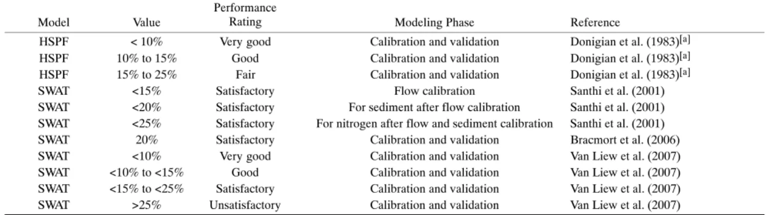
Table 3. Reported performance ratings for PBIAS.

Model Value PerformanceRating Modeling Phase Reference

HSPF < 10% Very good Calibration and validation Donigian et al. (1983)[a] HSPF 10% to 15% Good Calibration and validation Donigian et al. (1983)[a] HSPF 15% to 25% Fair Calibration and validation Donigian et al. (1983)[a]

SWAT <15% Satisfactory Flow calibration Santhi et al. (2001)

SWAT <20% Satisfactory For sediment after flow calibration Santhi et al. (2001) SWAT <25% Satisfactory For nitrogen after flow and sediment calibration Santhi et al. (2001) SWAT 20% Satisfactory Calibration and validation Bracmort et al. (2006) SWAT <10% Very good Calibration and validation Van Liew et al. (2007) SWAT <10% to <15% Good Calibration and validation Van Liew et al. (2007) SWAT <15% to <25% Satisfactory Calibration and validation Van Liew et al. (2007) SWAT >25% Unsatisfactory Calibration and validation Van Liew et al. (2007) [a] _{Adapted by Van Liew et al. (2003) and Singh et al. (2004).}

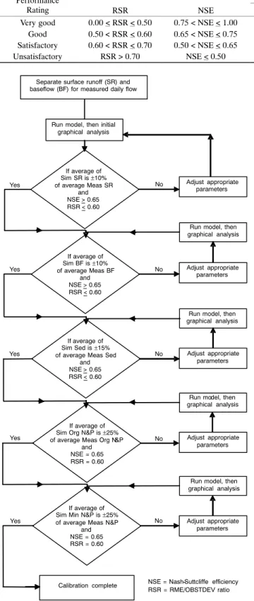
Table 4. General performance ratings for recommended statistics for a monthly time step. Performance

Rating RSR NSE

PBIAS (%)

Streamflow Sediment N, P

Very good 0.00 < RSR < 0.50 0.75 < NSE < 1.00 PBIAS < ±10 PBIAS < ±15 PBIAS< ±25 Good 0.50 < RSR < 0.60 0.65 < NSE < 0.75 ±10 < PBIAS < ±15 ±15 < PBIAS < ±30 ±25 < PBIAS < ±40 Satisfactory 0.60 < RSR < 0.70 0.50 < NSE < 0.65 ±15 < PBIAS < ±25 ±30 < PBIAS < ±55 ±40 < PBIAS < ±70 Unsatisfactory RSR > 0.70 NSE < 0.50 PBIAS > ±25 PBIAS > ±55 PBIAS > ±70

Separate surface runoff (SR) and baseflow (BF) for measured daily flow

NSE = Nash−Suttcliffe efficiency RSR = RME/OBSTDEV ratio Calibration complete Yes No No Yes No Yes Yes No No Yes

Run model, then initial graphical analysis

Adjust appropriate parameters

Run model, then graphical analysis

Run model, then graphical analysis

Run model, then graphical analysis

Run model, then graphical analysis Adjust appropriate parameters Adjust appropriate parameters Adjust appropriate parameters Adjust appropriate parameters If average of Sim SR is ±10% of average Meas SR and NSE > 0.65 RSR < 0.60 If average of Sim BF is ±10% of average Meas BF and NSE > 0.65 RSR < 0.60 If average of Sim Sed is ±15% of average Meas Sed

and NSE > 0.65 RSR < 0.60

If average of Sim Org N&P is ±25% of average Meas Org N&P

and NSE = 0.65 RSR = 0.60

If average of Sim Min N&P is ±25% of average Meas N&P

and NSE = 0.65 RSR = 0.60

Figure 1. General calibration procedure for flow, sediment, and nutrients in the watershed models (based on calibration chart for SWAT from San-thi et al., 2001).

The next step should be to calculate values for NSE, PBIAS, and RSR. With these values, model performance can be judged based on general performance ratings (table 4). The reported performance ratings and corresponding values developed for individual studies, in addition to the reported

ranges of values (table 1), were used to establish general per-formance ratings, which appear in table 4. As shown in table 4, the performance ratings for RSR and NSE are the same for all constituents, but PBIAS is constituent specific. This difference is due to the recent availability of information (PBIAS) on the uncertainty of measured streamflow and wa-ter quality. Harmel et al. (2006) used the root mean square er-ror propagation method of Topping (1972) to calculate the cumulative probable error resulting from four procedural categories (discharge measurement, sample collection, sam-ple preservation and storage, and laboratory analysis) associ-ated with water quality data collection. Under typical scenarios with reasonable quality control attention, typical financial and personnel resources, and typical hydrologic conditions, cumulative probable error ranges (in similar units to PBIAS) were estimated to be 6% to 19% for streamflow, 7% to 53% for sediment, and 8% to 110% for N and P. These results were used to establish constituent-specific perfor-mance rating for PBIAS. Constituent-specific ratings for RSR and NSE can be established when similar information becomes available.

Based on table 4, model performance can be evaluated as “satisfactory” if NSE > 0.50 and RSR < 0.70 and, for mea-sured data of typical uncertainty, if PBIAS ± 25% for stream-flow, PBIAS ± 55% for sediment, and PBIAS ± 70% for N and P for a monthly time step. These ratings should be adjusted to be more or less strict based on project-specific consider-ations discussed in the next section.

A general calibration procedure chart (fig. 1) for flow, sed-iment, and nutrients is included to aid with the manual model calibration process. The recommended values for adequate model calibration are within the “good” and “very good” per-formance ratings presented in table 4. These limits for ade-quate manual calibration are stricter than the “satisfactory” rating for general model evaluation because model parameter values are optimized during calibration but not during model validation or application. The importance of and appropriate methods for proper model calibration are discussed in the next section.

ADDITIONAL CONSIDERATIONS

The model evaluation guidelines presented in the previous section apply to the typical case of continuous, long-term simulation for a monthly time step. However, because of the diversity of modeling applications, these guidelines should be adjusted based on single-event simulation, quality and quantity of measured data, model calibration procedure, evaluation time step, and project scope and magnitude.

Single-Event Simulation

When watershed models are applied on a single-event ba-sis, evaluation guidelines should reflect this specific case. Generally, the objectives of single-event modeling are the de-termination of peak flow rate and timing, flow volume, and recession curve shape (ASCE, 1993; Van Liew et al., 2003).

Accurate prediction of peak flow rate and time-to-peak is es-sential for flood estimation and forecasting (Ramírez, 2000). Time-to-peak is affected by drainage network density, slope, channel roughness, and soil infiltration characteristics (Ramírez, 2000), and peak flow rate is typically affected by rainfall intensity and antecedent soil moisture content, among other factors.

One of the recommended (ASCE, 1993) model evaluation statistics for the peak flow rate is a simple percent error in peak flow rates (PEP) computed by dividing the difference between the simulated peak flow rate and measured peak flow rate by the measured peak flow rate and expressing the result as a percentage. Model performance related to time-to-peak can be determined similarly. In addition, for single-event simulation, Boyle et al. (2000) recommended that the hydrograph be divided into three phases (rising limb, falling limb, baseflow) based on differing watershed behavior dur-ing rainfall and dry periods. A different performance ratdur-ing should be applied to each hydrograph phase. If the mance ratings are similar for each phase, then a single perfor-mance rating can be applied to the overall hydrograph in subsequent evaluation. Otherwise, a different performance rating should be used to evaluate each hydrograph phase.

Quality and Quantity of Measured Data

Although it is commonly accepted that measured data are inherently uncertain, the uncertainty is rarely considered in model evaluation, perhaps because of the lack of relevant data. Harmel et al. (2006) suggested that the uncertainty of measured data, which varies based on measurement condi-tions, techniques, and constituent type, must be considered to appropriately evaluate watershed models. In terms of the present guidelines and performance ratings, modeled stream-flow may be rated “good” if it is within 10% to 15% of mea-sured streamflow data of typical quality (table 4), for example. In contrast, performance ratings should be stricter when high-quality (low uncertainty) data are available. In this case, PBIAS for modeled streamflow may be required to be <10% to receive a “good” rating. If data collected in worst-case conditions are used for model evaluation, then perfor-mance ratings should be relaxed to reflect the extreme uncertainty. It can be argued in this case, however, that highly uncertain data offer little value and should not be used in model evaluation.

Finally, in situations when a complete measured time se-ries does not exist, for instance when only a few grab samples per year are available, the data may not be sufficient for anal-ysis using the recommended statistics. In such situations, comparison of frequency distributions and/or percentiles (e.g., 10th, 25th, 50th, 75th, and 90th) may be more appropri-ate than the quantitative statistics guidelines.

Model Calibration Procedure

Proper model calibration is important in hydrologic mod-eling studies to reduce uncertainty in model simulations (En-gel et al., 2007). Ideal model calibration involves: (1) using data that includes wet, average, and dry years (Gan et al., 1997), (2) using multiple evaluation techniques (Willmott, 1981; ASCE, 1993; Legates and McCabe, 1999; Boyle et al., 2000), and (3) calibrating all constituents to be evaluated.

The calibration procedure typically involves a sensitivity analysis followed by manual or automatic calibration. The most fundamental sensitivity analysis technique utilizes par-tial differentiation, whereas the simplest method involves

perturbing parameter values one at a time (Hamby, 1994). A detailed review of sensitivity analysis methods is presented by Hamby (1994) and Isukapalli (1999). According to Isuka-palli (1999), the choice of a sensitivity method depends on the sensitivity measure employed, the desired accuracy in the estimates of the sensitivity measure, and the computational cost involved. Detailed information on how these factors af-fect the choice of sensitivity analysis method is given by Isu-kapalli (1999). After key parameters and their respective required precision have been determined, manual or auto-matic calibration is done.

Conventionally, calibration is done manually and consists of changing model input parameter values to produce simu-lated values that are within a certain range of measured data (Balascio et al., 1998). The calibrated model may be used to simulate multiple processes, such as streamflow volumes, peak flows, and/or sediment and nutrient loads. In such cases, two or more model evaluation statistics may be necessary in order to address the different processes (Balascio et al., 1998). However, when the number of parameters used in the manual calibration is large, especially for complex hydrolog-ic models, manual calibration can become labor-intensive (Balascio et al., 1998). In this, case automatic calibration is more appropriate.

Automatic calibration involves computation of the predic-tion error using an equapredic-tion (objective funcpredic-tion) and an auto-matic optimization procedure (search algorithm) to search for parameter values that optimize the value of the objective func-tion (Gupta et al., 1999). One of the automatic calibrafunc-tion meth-ods is the shuffled complex evolution global optimization algorithm developed at the University of Arizona (SCE-UA) (Duan et al., 1993) and used by vanGriensven and Bauwens (2003) to develop a multi-objective calibration method for semi-distributed water quality models. Other automatic calibra-tion methods include the multilevel calibracalibra-tion (MLC) semi-automated method (Brazil, 1988), the multi-objective complex evolution algorithm (MOCOM-UA) (Yapo et al., 1998), and pa-rameter estimation by sequential testing (PEST) (Taylor and Creelman, 1967), among others.

Data used to calibrate model simulations have a direct ef-fect on the validation and evaluation results. Ideal calibration should use 3 to 5 years of data that includes average, wet, and dry years so that the data encompass a sufficient range of hydrologic events to activate all model constituent processes during calibration (Gan et al., 1997). However, if this is not possible, then the available data should be separated into two sets, i.e., “above-mean” flows (wet years) and “below-mean” flows (dry years), and then evaluated with stricter perfor-mance ratings required for wet years (Gupta et al., 1999). Moreover, if the goal is to test the robustness of the model ap-plications under different environmental conditions, then dif-ferent datasets can be used during model calibration and validation.

In addition, a good calibration procedure uses multiple statistics, each covering a different aspect of the hydrograph, so that the whole hydrograph is covered. This is important be-cause using a single statistic can lead to undue emphasis on matching one aspect of the hydrograph at the expense of other aspects (Boyle et al., 2000). For manual calibration, each sta-tistic should be tracked while adjusting model parameters (Boyle et al., 2000) to allow for balancing the trade-offs in the ability of the model to simulate various aspects of the hydro-graph while recognizing potential errors in the observed data.

Finally, ideal model calibration considers water balance (peak flow, baseflow) and sediment and nutrient transport be-cause calibrating one constituent will not ensure that other constituents are adequately simulated during validation. Even though a complete set of hydrologic and water quality data are rarely available, all available data should be consid-ered. To calibrate water balance, it is recommended to sepa-rate baseflow and surface flow (surface runoff) from the total streamflow for both the measured and simulated data using a baseflow filter program. The baseflow filter developed by Arnold et al. (1995) and modified by Arnold and Allen (1999) is available at www.brc.tamus.edu/swat/soft_baseflow .html. Baseflow and recharge data from this procedure have shown good correlation with those produced by SWAT (Arnold et al., 2000). With estimated baseflow data, the baseflow ratio can be computed for measured and simulated data by divid-ing baseflow estimates by the total measured or simulated streamflow. The calibration and validation process can be considered satisfactory if the estimated baseflow ratio for simulated flow is within 20% of the measured flow baseflow ratio (Bracmort et al., 2006). Because plant growth and bio-mass production can have an effect on the water balance, rea-sonable local/regional plant growth days and biomass production may need to be verified during model calibration. Annual local/regional evapotranspiration (ET) may also need to be verified or compared with measured estimates dur-ing model calibration.

Stricter performance ratings should generally be required during model calibration than during validation. This differ-ence is recommended because parameter values are opti-mized during model calibration, but parameters are not adjusted in validation, which is possibly conducted under dif-ferent conditions than those occurring during calibration. Al-though the importance of model calibration is well established, performance ratings can be relaxed if improper calibration procedures are employed.

It is necessary to note that although proper model calibra-tion is important in reducing error in model output, experi-ence has shown that model simulation results may contain substantial errors. Therefore, rather than provide a point esti-mate of a given quantity of model output, it may be preferable to provide an interval estimate with an associated probability that the value of the quantity will be contained by the interval (Haan et al., 1998). In other words, uncertainty analysis needs to be included in model evaluations. Uncertainty analysis is defined as the process of quantifying the level of confidence in a given model simulation output based on: (1) the quality and amount of measured data available, (2) the absence of measured data due to the lack of monitoring in certain loca-tions, (3) the lack of knowledge about some physical pro-cesses and operational procedures, (4) the approximate nature of the mathematical equations used to simulate pro-cesses, and (5) the quality of the model sensitivity analysis and calibration. Detailed model uncertainty analysis is be-yond the scope of this research, but more model output uncer-tainty information can be obtained from published literature.

Evaluation Time Step

Most of the literature reviewed used daily and/or monthly time steps (Saleh et al., 2000; Santhi et al., 2001; Yuan et al., 2001; Sands et al., 2003; Van Liew et al., 2003; Chu and Shir-mohammadi, 2004; Saleh and Du, 2004; Singh et al., 2004; Bracmort et al., 2006; Singh et al., 2005; Van Liew et al.,

2007), although a few used annual time steps (Gupta et al., 1999; Shirmohammadi et al., 2001; Reyes et al., 2004), and one used weekly time steps (Narasimhan et al., 2005). There-fore, the time steps considered in this article are the daily and monthly. Typically, model simulations are poorer for shorter time steps than for longer time steps (e.g., daily versus monthly or yearly) (Engel et al., 2007). For example, Yuan et al. (2001) reported an R2 _{value of 0.5 for event comparison}

of predicted and observed sediment yields, and an R2 _value

of 0.7 for monthly comparison. The NSE values were 0.395 and 0.656 for daily and monthly, respectively, for DRAINMOD-DUFLOW calibration, and 0.363 and 0.664 for daily and monthly, respectively, for DRAINMOD-W cal-ibration (Fernandez et al., 2005). Similarly, the NSE values were 0.536 and 0.870 for daily and monthly, respectively, for DRAINMOD-DUFLOW validation, and 0.457 and 0.857 for daily and monthly, respectively, for DRAINMOD-W valida-tion (Fernandez et al., 2005). Addivalida-tional research work that supports the described findings includes that of Santhi et al. (2001), Van Liew et al. (2003), and Van Liew et al. (2007) us-ing SWAT. The performance ratus-ings presented in table 4 for RSR and NSE statistics are for a monthly time step; therefore, they need to be modified appropriately. Generally, as the evaluation time step increases, a stricter performance rating is warranted.

Project Scope and Magnitude

The scope and magnitude of the modeling project also af-fects model evaluation guidelines. The intended use of the model is an indication of the seriousness of the potential con-sequences or impacts of decisions made based on model re-sults (U.S. EPA, 2002). For instance, stricter performance rating requirements need to be set for projects that involve potentially large consequences, such as congressional testi-mony, development of new laws and regulations, or the sup-port of litigation. More modest performance ratings would be acceptable for technology assessment or “proof of principle,” where no litigation or regulatory action is expected. Even lower performance ratings will suffice if the model is used for basic exploratory research requiring extremely fast turn-around or high flexibility.

Finally, according to the U.S. EPA (2002), if model simu-lation does not yield acceptable results based on predefined performance ratings, this may indicate that: (1) conditions in the calibration period were significantly different from those in the validation period, (2) the model was inadequately or improperly calibrated, (3) measured data were inaccurate, (4) more detailed inputs are required, and/or (5) the model is unable to adequately represent the watershed processes of in-terest.

A C

S

PROJECT DESCRIPTION

As a component of the CEAP-WAS, the Soil and Water Assessment Tool (SWAT2005; Arnold et al., 1998) was ap-plied to the Leon River watershed in Texas. The watershed drains into Lake Belton, which lies within Bell and Coryell counties and provides flood control, water supply, and public recreation. The lake has a surface area of approximately 12,300 acres with a maximum depth of 124 feet. The total conservation storage is 372,700 ac-ft. The Lake Belton wa-tershed (Leon River) covers approximately 2.3 million acres

within five counties in central Texas. The majority of the land use in the watershed is pasture, hay, and brushy rangeland (63%). Cropland comprises about 10% of the watershed area. The northwestern (upper) half of the watershed contains nu-merous animal feeding operations, mainly dairies. Currently, there are approximately 60 permitted dairies and 40 smaller dairies (not requiring permits), with approximately 70,000 total cows. The main goal of the study is to use SWAT2005 to predict the impact of land management on the watershed over long periods of time, with special focus on waste man-agement practices.

To accomplish this goal, SWAT2005, with its many input parameters that describe physical, chemical, and biological processes, required calibration for application in the study watershed. Proper model calibration is important in hydro-logic modeling studies to reduce uncertainty in model predic-tions. For a general description of proper model calibration

procedures, refer to the previous discussion in the Additional Considerations section.

MODEL EVALUATION RESULTS BASEDONTHE DEVELOPED

GUIDELINES

When these model performance ratings were applied to the SWAT2005 modeling in the Leon River (Lake Belton) watershed, the following results were obtained (figs. 2 and 3, table 5). Graphical results during calibration (fig. 2) and val-idation (fig. 3) indicated adequate calibration and valval-idation over the range of streamflow, although the calibration results showed a better match than the validation results. NSE values for the monthly streamflow calibration and validation ranged from 0.66 to 1.00. According to the model evaluation guide-lines, SWAT2005 simulated the streamflow trends well to very well, as shown by the statistical results, which are in agreement with the graphical results. The RSR values ranged

Figure 2. Monthly discharge (CMS) calibration for the Leon River sub-basin 6 WS outlet.

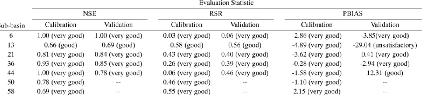
Table 5. Results of SWAT2005 average monthly streamflow model output, Leon River watershed, Texas, based on the developed model evaluation guidelines.

Sub-basin

Evaluation Statistic

NSE RSR PBIAS

Calibration Validation Calibration Validation Calibration Validation 6 1.00 (very good) 1.00 (very good) 0.03 (very good) 0.06 (very good) -2.86 (very good) -3.85(very good) 13 0.66 (good) 0.69 (good) 0.58 (good) 0.56 (good) -4.89 (very good) -29.04 (unsatisfactory) 21 0.81 (very good) 0.84 (very good) 0.43 (very good) 0.40 (very good) -3.62 (very good) 0.41 (very good) 36 0.93 (very good) 0.85 (very good) 0.26 (very good) 0.39 (very good) -0.28 (very good) -2.94 (very good) 44 1.00 (very good) 0.78 (very good) 0.06 (very good) 0.46 (very good) -1.58 (very good) 12.31 (good)

50 0.78 (very good) -- 0.46 (very good) -- -1.10 (very good)

--58 0.69 (very good) -- 0.55 (very good) -- 2.15 (very good)

--from 0.03 to 0.58 during both calibration and validation. These values indicate that the model performance for stream-flow residual variation ranged from good to very good. The PBIAS values varied from −4.89% to 2.15% during calibra-tion and from −29.04% to 12.31% during validation. The av-erage magnitude of simulated monthly streamflow values was within the very good range (PBIAS < ±10) for each sub-basin during calibration (table 5). However, simulated values fell within unsatisfactory, good, and very good ranges during validation for various sub-basins. Aside from one indication of unsatisfactory model performance, SWAT2005 simulation of streamflow was “good” to “very good” in terms of trends (NSE), residual variation (RSR), and average magnitude (PBIAS). As apparent from this evaluation of the Leon River watershed, situations might arise that generate conflicting performance ratings for various watersheds and/or output variables.

In situations with conflicting performance ratings, those differences must be clearly described. For example, if simu-lation for one output variable in one watershed produces un-balanced performance ratings of “very good” for PBIAS, “good” for NSE, and “satisfactory” for RSR, then the overall performance should be described conservatively as “satisfac-tory” for that one watershed and that one output variable. However, it would be preferable to describe the performance in simulation of average magnitudes (PBIAS) as “very good,” in simulation of trends (NSE) as “good,” and in simu-lation of residual variation (RSR) as “satisfactory.” Similarly, if performance ratings differ for various watersheds and/or output types, then those differences must be clearly de-scribed.

S

C

Most research and application projects involving wa-tershed simulation modeling utilize some type of predefined, project-specific model evaluation techniques to compare simulated output with measured data. Previous research has produced valuable comparative information on selected model evaluation techniques; however, no comprehensive standardization is available that includes recently developed statistics with corresponding performance ratings and appli-cable guidelines for model evaluation. Thus, the present re-search selected and recommended model evaluation techniques (graphical and statistical), reviewed published ranges of values and corresponding performance ratings for the recommended statistics, and established guidelines for model evaluation based on the review results and project-specific considerations. These recommendations and

discus-sion apply to evaluation of model simulation related to streamflow, sediments, and nutrients (N and P).

Based on previous published recommendations, a com-bination of graphical techniques and dimensionless and error index statistics should be used for model evaluation. In addi-tion to hydrographs and percent exceedance probability curves, the quantitative statistics NSE, PBIAS, and RSR were recommended. Performance ratings for the recom-mended statistics, for a monthly time step, are presented in table 4. In general, model simulation can be judged as “satis-factory” if NSE > 0.50 and RSR < 0.70, and if PBIAS ± 25% for streamflow, PBIAS ± 55% for sediment, and PBIAS

± 70% for N and P for measured data of typical uncertainty. These PBIAS ratings, however, should be adjusted if mea-surement uncertainty is either very low or very high. As indi-cated by these PBIAS ratings, it is important to consider measured data uncertainty when using PBIAS to evaluate watershed models. In addition, general guidelines for manual calibration for flow, sediment, and nutrients were presented (fig. 1). Additional considerations, such as single-event sim-ulation, quality and quantity of measured data, model cal-ibration procedure considerations, evaluation time step, and project scope and magnitude, which affect these guidelines, were also discussed. The guidelines presented should be ad-justed when appropriate to reflect these considerations. To il-lustrate the application of the developed model evaluation guidelines, a case study was provided.

Finally, the recommended model evaluation statistics and their respective performance ratings, and the step-by-step de-scription of how they should be used, were presented together to establish a platform for model evaluation. As new and im-proved methods and information are developed, the recom-mended guidelines should be updated to reflect these developments.

ACKNOWLEDGEMENTS

The USDA-NRCS is acknowledged for providing funds for this work through the support of the Conservation Effects As-sessment Project − Watershed Assessment Studies. The authors are grateful to Tim Dybala for allowing the use of part of his work for the case study. The authors also thank Alan Verser for additional information on model calibration procedure.

R

Amatya, D. M., G. M. Chescheir, G. P. Fernandez, R. W. Skaggs, and J. W. Gilliam. 2004. DRAINWAT-based methods for esti-mating nitrogen transport in poorly drained watersheds. Trans. ASAE 47(3): 677-687.

Arnold, J. G., and P. M. Allen. 1999. Automated methods for esti-mating baseflow and ground water recharge from streamflow re-cords. J. American Water Resources Assoc. 35(2): 411-424. Arnold, J. G., P. M. Allen, R. Muttiah, and G. Bernhardt. 1995.

Au-tomated base flow separation and recession analysis techniques.

Ground Water 33(6): 1010-1018.

Arnold, J. G., R. Srinivisan, R. S. Muttiah, and P. M. Allen. 1998. Large-area hydrologic modeling and assessment: Part I. Model development. J. American Water Resources Assoc. 34(1): 73-89. Arnold, J. G., R. S. Muttiah, R. Srinivasan, and P. M. Allen. 2000.

Regional estimation of base flow and groundwater recharge in the upper Mississippi River basin. J. Hydrology 227(1-2): 21-40. ASCE. 1993. Criteria for evaluation of watershed models. J.

Irriga-tion Drainage Eng. 119(3): 429-442.

Balascio, C. C., D. J. Palmeri, and H. Gao. 1998. Use of a genetic algorithm and multi-objective programming for calibration of a hydrologic model. Trans. ASAE 41(3): 615-619.

Borah, D. K., and M. Bera. 2004. Watershed-scale hydrologic and nonpoint-source pollution models: Review of applications.

Trans. ASAE 47(3): 789-803.

Boyle, D. P., H. V. Gupta, and S. Sorooshian. 2000. Toward im-proved calibration of hydrologic models: Combining the strengths of manual and automatic methods. Water Resources Res. 36(12): 3663-3674.

Bracmort, K. S., M. Arabi, J. R. Frankenberger, B. A. Engel, and J. G. Arnold. 2006. Modeling long-term water quality impact of structural BMPS. Trans. ASAE 49(2): 367-384.

Brazil, L. E. 1988. Multilevel calibration strategy for complex hydrologic simulation models. Unpublished PhD diss. Fort Col-lins, Colo.: Colorado State University, Department of Civil En-gineering.

CEAP-WAS. 2005. Conservation effects assessment project: Wa-tershed assessment studies. Available at:

ftp://ftp-fc.sc.egov.usda.gov/NHQ/nri/ceap/ceapwaswebrev121004.pdf. Accessed 15 August 2005.

Chu, T. W., and A. Shirmohammadi. 2004. Evaluation of the SWAT model’s hydrology component in the piedmont physiographic region of Maryland. Trans. ASAE 47(4): 1057-1073.

Donigian, A. S., J. C. Imhoff, and B. R. Bicknell. 1983. Predicting wa-ter quality resulting from agricultural nonpoint-source pollution via simulation − HSPF. In Agricultural Management and Water Quali-ty, 200-249. Ames, Iowa: Iowa State University Press.

Duan, Q. Y., V. K Gupta, and S. Sorooshian. 1993. Shuffled com-plex evolution approach for effective and efficient global mini-mization. J. Optimization Theory and Appl. 76(3): 501-521. Engel B., D. Storm, M. White, and J. G. Arnold. 2007. A

hydrolog-ic/water quality model application protocol. J. American Water Resources Assoc. (in press).

Engelmann, C. J. K, A. D. Ward, A. D. Christy, and E. S. Bair. 2002. Applications of the BASINS database and NPSM model on a small Ohio watershed. J. American Water Resources Assoc.

38(1): 289-300.

Fernandez, G. P., G. M. Chescheir, R. W. Skaggs, and D. M. Ama-tya. 2005. Development and testing of watershed-scale models for poorly drained soils. Trans. ASAE 48(2): 639-652. Gan, T. Y., and G. F. Biftu. 1996. Automatic calibration of

concep-tual rainfall-runoff models: Optimization algorithms, catchment conditions, and model structure. Water Resources Res. 32(12): 3513-3524.

Gan, T. Y, E. M. Dlamini, and G. F. Biftu. 1997. Effects of model complexity and structure, data quality, and objective functions on hydrologic modeling. J. Hydrology 192(1): 81-103. Gupta, H. V., S. Sorooshian, and P. O. Yapo. 1999. Status of

auto-matic calibration for hydrologic models: Comparison with mul-tilevel expert calibration. J. Hydrologic Eng. 4(2): 135-143. Haan, C. T., D. E. Storm, T. Al-Issa, S. Prabhu, G. J. Sabbagh, and

D. R. Edwards. 1998. Effect of parameter distributions on uncer-tainty analysis of hydrologic models. Trans. ASAE 41(1): 65-70.

Hamby, D. M. 1994. A review of techniques for parameter sensitiv-ity analysis of environmental models. Environ. Monitoring and Assessment 32(2): 135-154.

Harmel, R. D., R. J. Cooper, R. M. Slade, R. L. Haney, and J. G. Ar-nold. 2006. Cumulative uncertainty in measured streamflow and water quality data for small watersheds. Trans. ASAE 49(3): 689-701.

Isukapalli, S. S. 1999. Uncertainty analysis of

transport-transformation models. Unpublished PhD diss. New Brunswick, N.J.: Rutgers, The State University of New Jersey, Department of Chemical and Biochemical Engineering.

Legates, D. R., and G. J. McCabe. 1999. Evaluating the use of “goodness-of-fit” measures in hydrologic and hydroclimatic model validation. Water Resources Res. 35(1): 233-241. Ma, L., J. C. Ascough II, L. R. Ahuja, M. J. Shaffer, J. D. Hanson,

and K. W. Rojas. 2000. Root zone water quality model sensitiv-ity analysis using Monte Carlo simulation. Trans. ASAE 43(4): 883-895.

Motovilov, Y. G., L. Gottschalk, K. England, and A. Rodhe. 1999. Validation of distributed hydrological model against spatial ob-servations. Agric. Forest Meteorology 98-99: 257-277. Narasimhan, B., R. Srinivasan, J. G. Arnold, and M. Di Luzio.

2005. Estimation of long-term soil moisture using a distributed parameter hydrologic model and verification using remotely sensed data. Trans. ASAE 48(3): 1101-1113.

Nash, J. E., and J. V. Sutcliffe. 1970. River flow forecasting through conceptual models: Part 1. A discussion of principles. J. Hydrol-ogy 10(3): 282-290.

Parker, R., J. G. Arnold, M. Barrett, L. Burns, L. Carrubba, C. Crawford, S. L. Neitsch, N. J. Snyder, R. Srinivasan, and W. M. Williams. 2006. Evaluation of three watershed-scale pesticide fate and transport models. J. American Water Resources Assoc.

(in review).

Peterson, J. R., and J. M. Hamlett. 1998. Hydrologic calibration of the SWAT model in a watershed containing fragipan soils. J. American Water Resources Assoc. 34(3): 531-544.

Ramanarayanan, T. S., J. R. Williams, W. A. Dugas, L. M. Hauck, and A. M. S. McFarland. 1997. Using APEX to identify alterna-tive practices for animal waste management. ASAE Paper No. 972209. St. Joseph, Mich.: ASAE.

Ramírez, J. A. 2000. Chapter 11: Prediction and modeling of flood hydrology and hydraulics. In Inland Flood Hazards: Human, Riparian and Aquatic Communities. E. Wohl, ed. Cambridge, U.K.: Cambridge University Press.

Reyes, M. R., R. W. Skaggs, and R. L. Bengtson. 2004. GLEAMS-SWT with nutrients. Trans. ASAE 47(1): 129-132.

Refsgaard, J. C. 1997. Parameterisation, calibration, and validation of distributed hydrological models. J. Hydrology 198(1): 69-97. Saleh, A., and B. Du. 2004. Evaluation of SWAT and HSPF within BASINS program for the upper North Bosque River watershed in central Texas. Trans. ASAE 47(4): 1039-1049.

Saleh, A, J. G. Arnold, P. W. Gassman, L. M. Hauk, W. D. Rosen-thal, J. R. Williams, and A. M. S. MacFarland. 2000. Applica-tion of SWAT for the upper North Bosque River watershed.

Trans. ASAE 43(5): 1077-1087.

Sands, G. R., C. X. Jin, A. Mendez, B. Basin, P. Wotzka, and P. Gowda. 2003. Comparing the subsurface drainage flow predic-tion of the DRAINMOD and ADAPT models for a cold climate.

Trans. ASAE 46(3): 645-656.

Santhi, C, J. G. Arnold, J. R. Williams, W. A. Dugas, R. Srinivasan, and L. M. Hauck. 2001. Validation of the SWAT model on a large river basin with point and nonpoint sources. J. American Water Resources Assoc. 37(5): 1169-1188.

Sevat, E., and A. Dezetter. 1991. Selection of calibration objective functions in the context of rainfall-runoff modeling in a Suda-nese savannah area. Hydrological Sci. J. 36(4): 307-330. Shirmohammadi, A., T. W. Chu, H. Montas, and T. Sohrabi. 2001.

pollution assessment. ASAE Paper No. 012005. St. Joseph, Mich.: ASAE.

Singh, J., H. V. Knapp, and M. Demissie. 2004. Hydrologic model-ing of the Iroquois River watershed usmodel-ing HSPF and SWAT. ISWS CR 2004-08. Champaign, Ill.: Illinois State Water Survey. Available at: www.sws.uiuc.edu/pubdoc/CR/

ISWSCR2004-08.pdf. Accessed 8 September 2005. Singh, J., H. V. Knapp, J. G. Arnold, and M. Demissie. 2005.

Hydrologic modeling of the Iroquois River watershed using HSPF and SWAT. J. American Water Resources Assoc. 41(2): 361-375.

Spruill, C. A., S. R. Workman, and J. L. Taraba. 2000. Simulation of daily and monthly stream discharge from small watersheds using the SWAT model. Trans. ASAE 43(6): 1431-1439. Taylor, M. M., and C. D. Creelman. 1967. PEST: Efficient estimates

on probability functions. J. Acoustical Soc. America 41(4A): 782-787.

Topping, J. 1972. Errors of Observation and Their Treatment. 4th ed. London, U.K.: Chapman and Hall.

U.S. EPA. 2002. Guidance for quality assurance project plans for modeling. EPA QA/G-5M. Report EPA/240/R-02/007. Wash-ington, D.C.: U.S. EPA, Office of Environmental Information. vanGriensven, A., and W. Bauwens. 2003. Multiobjective

autocal-ibration for semidistributed water quality models. Water Re-sources Res. 39(12): 1348-1356.

Van Liew, M. W., J. G. Arnold, and J. D. Garbrecht. 2003. Hydro-logic simulation on agricultural watersheds: Choosing between two models. Trans. ASAE 46(6): 1539-1551.

Van Liew, M. W., T. L. Veith, D. D. Bosch, and J. G. Arnold. 2007. Suitability of SWAT for the conservation effects assessment project: A comparison on USDA-ARS experimental watersheds.

J. Hydrologic Eng. 12(2): 173-189.

Varanou, E., E. Gkouvatsou, E. Baltas, and M. Mimikou. 2002. Quantity and quality integrated catchment modeling under cli-mate change with use of soil and water assessment tool model.

ASCE J. Hydrologic Eng. 7(3): 228-244.

Vazquez-Amábile, G. G., and B. A. Engel. 2005. Use of SWAT to compute groundwater table depth and streamflow in the Musca-tatuck River watershed. Trans. ASAE 48(3): 991-1003. Wang, X., and A. M. Melesse. 2005. Evaluation of the SWAT

mod-el’s snowmelt hydrology in a northwestern Minnesota wa-tershed. Trans. ASAE 48(4): 1359-1376.

Willmott, C. J. 1984. On the evaluation of model performance in physical geography. In Spatial Statistics and Models, 443-460. G. L. Gaile and C. J. Willmott, eds. Norwell, Mass.: D. Reidel. Willmott, C. J. 1981. On the validation of models. Physical

Geog-raphy 2: 184-194.

Yapo, P. O., H. V. Gupta, and S. Sorooshian, 1998. Multi-objective global optimization for hydrologic models. J. Hydrology 204(1): 83-97.

Yuan, Y., R. L. Bingner, and R. A. Rebich. 2001. Evaluation of An-nAGNPS on Mississippi Delta MSEA watersheds. Trans. ASAE

44(5): 1183-1190.

A

Reported Values of NSE and PBIAS for Various Constituents

Table A-1. Daily and monthly surface runoff calibration and validation value ranges.[a]

Watershed - Model (Reference)

Calibration Value Ranges Validation Value Ranges

Statistic Daily Monthly Daily Monthly

Warner Creek, Maryland - SWAT Chu and Shirmohammadi, 2004)

NSE -- 0.35 -- 0.77

PBIAS Black Creek, Indiana - SWAT

(Bracmort et al., 2006)

NSE -- 0.62 to 0.80 -- 0.63 to 0.75

PBIAS

[a] _{In tables A-1 through A-9, a dash (--) indicates no value reported for the statistic used; a blank space indicates that the statistic was not used.} Table A-2. Daily and monthly sediment calibration and validation value ranges.

Watershed - Model (Reference)

Calibration Value Ranges Validation Value Ranges

Statistic Daily Monthly Daily Monthly

Bosque River, Texas - SWAT (Saleh et al., 2000)

NSE -- -- -- 0.81

PBIAS Bosque River, Texas - SWAT

(Santhi et al., 2001)

NSE -- 0.69 to 0.80 -- 0.23 to 0.70

PBIAS Bosque River, Texas - SWAT

(Saleh and Du, 2004)

NSE -2.50 0.83 -3.51 0.59

PBIAS Bosque River, Texas - HSPF

(Saleh and Du, 2004)

NSE 0.11 0.72 0.23 0.88

PBIAS Hellbranch Run, Ohio - HSPF

(Engelmann et al., 2002)[a]

NSE -- 0.49 -- -2.46

PBIAS Black Creek, Indiana - SWAT

(Bracmort et al., 2006)

NSE -- 0.86 to 0.92 -- 0.68 to 0.75

PBIAS [a] _{In Borah and Bera (2004).}