A Perfect Example for The BFGS Method
∗
Yu-Hong Dai
†Abstract
Consider the BFGS quasi-Newton method applied to a general non-convex function that has continuous second derivatives. This paper aims to construct a four-dimensional example such that the BFGS method need not converge. The example is perfect in the following sense: (a) All the stepsizes are exactly equal to one; the unit stepsize can also be accepted by various line searches including the Wolfe line search and the Arjimo line search; (b) The objective function is strongly convex along each search direction although it is not in itself. The unit stepsize is the unique minimizer of each line search function. Hence the example also applies to the global line search and the line search that always picks the first local minimizer; (c) The objective function is polynomial and hence is infinitely continuously differentiable. If relaxing the convexity requirement of the line search function; namely, (b), we are able to construct a relatively simple polynomial example.
Keywords. unconstrained optimization, quasi-Newton method, non-convex function, global convergence.
1
Introduction
Consider the unconstrained optimization problem
minf(x), x∈ Rn, (1.1) wherefis a general non-convex function that has continuous second derivatives. The quasi-Newton method is a class of well-known and efficient methods for solving (1.1). It is of the iterative scheme
xk+1=xk−αkHkgk, (1.2) ∗This work was partially supported by the Chinese NSF grants 10571171 and 10831106
and the CAS grant kjcx-yw-s7-03.
†State Key Laboratory of Scientific and Engineering Computing, Institute of
Computation-al Mathematics and Scientific/Engineering Computing, Academy of Mathematics and Systems Science, Chinese Academy of Sciences, P.O. Box 2719, Beijing 100190, P.R. China. E-mail:
wherex1 is a starting point,Hk is some approximation to the inverse Hessian [∇2f(xk)]−1,g
k =∇f(xk), andαkis a stepsize obtained in some way. Defining the vectors
δk=xk+1−xk, γk=gk+1−gk,
the quasi-Newton method asks the next approximation matrixHk+1 to satisfy the secant equation
Hk+1γk =δk. (1.3)
This similarity to the identical equation [∇2f(x
k+1)]−1γk=δk in the quadrat-ic case enables the quasi-Newton method to be superlinearly convergent (see Dennis and Mor´e [5], for example) and makes it very attractive in practical optimization.
The first quasi-Newton method was dated back to Davidon [4] and Fletcher and Powell [9]. The DFP method updates the approximation matrix Hk to Hk+1 by the formula Hk+1=Hk−Hkγkγ T kHk γTkHkγk + δkδ T k δTkγk. (1.4) Nowadays, the most efficient quasi-Newton method is perhaps the BFGS method, which was proposed by Broyden [2], Fletcher [7], Goldfarb [10], and Shanno [24], independently. The matrixHk+1 in the BFGS method can be updated by the way Hk+1=Hk−δkγ T kHk+Hkγkδ T k δTkγk + 1 + γ T kHkγk δTkγk δkδT k δTkγk. (1.5) To pass the positive definiteness of the matrixHk toHk+1, practical quasi-Newton algorithms make use of the Wolfe line search to calculate the stepsize αk, which ensures a positive curvature to be found at each iteration; namely, δTkγk >0. More exactly, defining the one-dimensional line search function
Ψk(α) =f(xk−αHkgk), α≥0, (1.6) the Wolfe line search consists in finding a stepsizeαk such that
Ψk(αk)≤Ψk(0) +µΨ0k(0)αk (1.7) and
Ψ0k(αk)≥ηΨ0k(0), (1.8) whereµandη are constants with 0< µ≤η <1.
There have been a large quantity of research works devoting to the global convergence of the quasi-Newton method (see Yuan [28] and Sun and Yuan [26], for example). Specifically, Powell [18] showed that the DFP method with exact line searches is globally convergent for uniformly convex functions. In another paper [20], Powell established the global convergence of the BFGS method with the Wolfe line search for uniformly convex functions. This result was extended
by Byrd, Nocedal and Yuan [1] to the whole Broyden’s convex family of methods except the DFP method. Therefore it is natural to ask the following question: Does the DFP method with the Wolfe line search converge globally for uniformly convex functions? On the other hand, since the BFGS method with the Wolfe line search works well for both convex and non-convex functions, we might ask another question: Does the BFGS method with the Wolfe line search converge globally for general functions? The difficulty and importance of the two conver-gence problems has been addressed in many situations, including Nocedal [15], Fletcher [8], and Yuan [28].
Recent studies provide a negative answer to the convergence problem of the BFGS method for nonconvex functions. As a matter of fact, in an early paper [21], which analyzes the convergence properties of the conjugate gradient method, Powell mentioned that the BFGS method need not converge if the line search can pick any local minimizer of the line search function Ψk(α). After further studies on the two-dimensional example in [21], Dai [3] presented an example with six cycling points and showed by the example that the BFGS method with the Wolfe line search may fail for nonconvex functions. Later, Mascarenhas [14] constructed a three-dimensional counter-example such that the BFGS method does not converge if the line search picks the global minimizer of the function Ψk(α). It should be noted that the stepsize in the counter-example of [14] also satisfies the Wolfe line search conditions. However, neither examples are such that the stepsize is the first local minimizer of the line search function Ψk(α).
Surprisingly enough, if there are only two variables, and if the stepsize is chosen to be the first local minimizer of Ψk(α); namely,
αk = arg min{α >0 : αis a local minimizer of Ψk(α)}, (1.9) Powell [22] established the global convergence of the BFGS method for general twice continuously differentiable function. Powell’s proof makes use of the prin-ciple of contradiction and is quite sophisticated. Assuming the nonconvergence of the method and the relation lim inf
k→∞ kgkk 6= 0, Powell showed that the limit points of the BFGS path
P ={x: xlies on the line segment connectingxk and xk+1 for somek≥1} (that is exactly the same as the Polak-Ribi`ere conjugate gradient path ifn= 2 andgTk+1δk = 0 for all k) forms some line segmentL. The use of the specific line search (1.9) is such that the objective function is monotonically decreasing on the line segment Lk that connects xk and xk+1. It follows that f(x) ≡
lim
k→∞f(xk) for all x ∈ L. Consequently, the line segment Lk cannot cross L and all the pointsxk with large indices lies in the same side ofL. Furthermore, Powell showed that starting around from one end of the line segment L, the BFGS path can not get any close to the other end ofL and finally obtained a contradiction. Intuitively, it is difficult to extend Powell’s result to the case when n≥ 3. This is because, even if it has been shown that the BFGS path
tends to some limit line segmentL, each line segment Lk could turn aroundL providing thatn≥3, making the similar analysis of the BFGS path complicated and nearly impossible.
The purpose of this paper is to construct a four-dimensional counter-example for the BFGS method with the following features:
(a) All the stepsizes in the example are exactly equal to one; namely,
αk ≡1; (1.10)
For the search direction defined by the BFGS update in the example, a unit stepsize satisfies various line search conditions, including the Wolfe conditions and the Armijo conditions;
(b) The objective function is strongly convex along each search direction; name-ly, the line search functionΨk(α)is strongly convex for allk, although the objective function is not in itself. The unit stepsize is the unique minimiz-er ofΨk(α). Hence the example also applies to the global line search and the specific line search (1.9);
(c) The objective function is polynomial and hence is infinitely continuously differentiable.
On the other hand, the objective function in our example is linear in the third and fourth variables and thus has no local minimizer. However, the iterations generated by the BFGS method tend to a non-stationary point.
As seen from§3.4, the construction of the example is quite complicated. To be such that the line search function Ψk(α) is strongly convex, a polynomial of degree 38 is introduced. Nevertheless, if we relax the convexity requirement of Ψk(α); namely, (b) in the above, it is possible to construct a relatively simple polynomial example of low degree (see§3.3).
The construction of our examples can be divided into four procedures: (1) Prefix the special forms of the steps{δk} and gradients{gk}, leaving several parameters to be determined later. In this case, once x1 is given, the whole sequence {xk} is fixed. As seen in §2.1, our steps {δk} and gradients {gk} are asked to possess some symmetrical and cyclic properties and to push the iterations {xk} tend to the eight vertices of a regular octagon. This is very helpful in simplifying the construction of the examples and we can focus our attention on the choice of the parameter t, that answers for the decay of the last two components ofδk and the first two components ofgk. (2) To enable the BFGS method to generate those prefixed steps, investigate the consistency conditions on the steps{δk} and gradients {gk}. With the prefixed forms of
{δk}and{gk}, we show in§2.2 that the unit stepsize is indispensable, whereas this stepsize is usually used as the first trial stepsize in the implementation of quasi-Newton methods. Four more consistency conditions on {δk} and {gk} are obtained in§2.3 by expressing the vectors Hk+1γk, Hk+1gk+1, Hk+1gk+2 andHk+1gk+3 by someδk’s and gk’s instead of considering the quasi-Newton
matrixHk+1 itself. (3) Choose the parameters in some way to satisfy the con-sistency conditions and other necessary conditions on the objective function. As seen in§2.4, the first three consistency conditions are actually corresponding to some under-determined linear system. Substituting its general solution by the Cramer’s rule into the fourth consistency condition, we are led to a nonlinear equation from which the exact value can be obtained for the decay parametert. By suitably choosing the other parameters, we can express all the quasi-Newton updating matrices including the initial choice for H1 in §2.5. (4) Construct a suitable objective functionf whose gradients are the preassigned values; name-ly, ∇f(xk) = gk for all k ≥1 and the line search has the desired properties. This will be done in the whole third section. To make full use of symmetrical and cyclic properties of the steps{δk} and{gk}, we carefully choose a special form of the objective function. In addition, the introduction of element func-tionφin §3.4 helps us greatly to convexify the line search function and finally complete the perfect example that meets all the requirements (a), (b) and (c). Some concluding remarks are given in the last section.
2
Looking for Consistent Steps and Gradients
2.1
The Forms of Steps and Gradients
Consider the case of four dimension. Inspired by [21], [3] and [14], we assume that the steps{δk} have the following form:
δ1= (η1, ξ1, γ1, τ1)T; δk+1=Mδk (k≥1), (2.1) whereM is the 4×4 matrix defined by
M = cosθ1 −sinθ1 sinθ1 cosθ1 0 0 t cosθ2 −sinθ2 sinθ2 cosθ2 . (2.2)
In the above,tis a parameter satisfying 0<|t|<1. This parameter answers for the decay of the last two components of the steps{δk}. The anglesθ1 and θ2 are chosen so thatθ1= m2π
1 andθ2 =
2π
m2 for some positive integersm1 and
m2. Specifically, we choose in this paper θ1=1
4π, θ2= 3
4π. (2.3)
Consequently, the first two components of the steps{δk}turn to the same after every eight iterations, and the last two components will shrink at a factor oft8 after every eight iterations. Further, we can see that the iterations {xk} will tend to turn around the eight vertices of some regular octagon (see§3.1 for more details).
Accordingly, the gradients{gk}are assumed to be of the form
where P = t cosθ1 −sinθ1 sinθ1 cosθ1 0 0 cosθ2 −sinθ2 sinθ2 cosθ2 . (2.5)
Since 0<|t|<1, we see that the first two components of{gk}vanish, whereas the last two components of the gradient {gk}, turn to the same after eight iterations. It follows that none of the cluster points generated by the BFGS method are stationary points.
2.2
Unit Stepsizes
It is well known that the unit stepsize is usually used as the first trial stepsize in practical implementations of the BFGS method. Under suitable assumptions on f, the unit stepsize will be accepted by the line search as the iterates tend to the solution and will enable a superlinear convergence step (see [5], for example). In the following, we are going to show that if the line search satisfies
gk+1T δk = 0, for allk≥1, (2.6) and if the steps generated by the BFGS method have the form (2.1)-(2.2) and the gradients have the form (2.4)-(2.5), then the use of unit stepsizes is also indispensable.
To begin with, we see that the line search condition (2.6), the secant equation (1.3) and the definition of the search direction
Hk+1gk+1=−α−k+11 δk+1 (2.7) indicate that
δTk+1γk=−αk+1gk+1T Hk+1γk =−αk+1gTk+1δk= 0. (2.8) The above relation (2.8) is sometimes called as theconjugacy conditionin the context of nonlinear conjugate gradient methods.
By multiplying the BFGS updating formula (1.5) withgk+1 and using (2.6), Hk+1gk+1=Hkgk+1−
γT
kHkgk+1 δTkγk
δk,
which with (2.7) gives
Hkgk+1=−α−k+11 δk+1+ γT kHkgk+1 δTkγk δk. (2.9) Multiplying (2.9) bygT
k and noticinggTkHkgk+1= 0, we get that
0 =−α−k+11 gTkδk+1+ γT kHkgk+1 δTkγk gkTδk=−α−k+11 g T kδk+1−γTkHkgk+1.
ThusγTkHkgk+1=−α−k+11 g T kδk+1=−α −1 k+1g T k+1δk+1. Hence, by (2.9), Hkgk+1=−α−k+11 δk+1−α −1 k+1 gTk+1δk+1 δTkγk δk. (2.10) It follows from (2.10) and (2.7) withkreplaced byk−1 that
Hkγk=−α− 1 k+1δk+1+ " α−k1−α−k+11 g T k+1δk+1 δTkγk # δk. (2.11)
Further, substituting this into the BFGS updating formula (1.5) yields
Hk+1=Hk+α−k+11 δkδTk+1+δk+1δ T k δTkγk + " 1−α−k1+α−k+11 g T k+1δk+1 δTkγk # δkδTk δTkγk . (2.12) The above new updating formula requires the quantity δk+1, that depends on Hk+1 itself, and hence has theoretical meanings only.
Lemma 2.1. Assume that (2.6) holds. Then for allk≥1andi≥0, the vector Hkgk+i+α−k+i1 δk+i belongs to the subspace spanned by δk, δk+1, . . ., δk+i−1; namely,
Hkgk+i+α−k+i1δk+i∈Span{δk,δk+1, . . . ,δk+i−1}. (2.13) Proof. For convenience, we write (2.12) as
Hk+1=Hk+V(sk,sk+1), (2.14) whereV(sk,sk+1) means the rank-two matrix in the right hand of (2.12). There-fore we have for alli≥1,
Hk+i=Hk+ i
X
j=1
V(sk+j−1,sk+j). (2.15)
The statement follows by multiplying the above relation with gk+i and using (2.7) withk replaced byk+i−1 andgT
k+iδk+i−1= 0. Q.E.D.
Lemma 2.2. To construct a desired example with Det(S1)6= 0, we must have that
αk= 1, for allk≥4. Proof. Define the following matrices
Gk = γk−1 gk gk+1 gk+2, Sk = δk−1 δk δk+1 δk+2 .
ByHkγk−1=δk−1and Lemma 2.1, we can get that
Det(Hk) Det(Gk) = DetHkγk−1 Hkgk Hkgk+1 Hkgk+2
= Detδk−1 −α−k1δk −α −1 k+1δk+1 −α −2 k+2δk+2 = −α−k1αk+1−1 α−k+21 Det(Sk). (2.16) Replacingkwithk+ 1 in the above yields
Det(Hk+1) Det(Gk+1) =−α−k+11 α−k+21 αk+3−1 Det(Sk+1). (2.17) On the other hand, due to the special forms of{gk}and{δk}, we know that Gk+1=P Gk andSk+1=M Sk. Hence
Det(Gk+1) = Det(P) Det(Gk) = t2Det(Gk),
Det(Sk+1) = Det(M) Det(Sk) = t2Det(Sk). (2.18)
Due to the basic determinant relation of the BFGS update, (2.6) and (2.7), it is not difficult to see that
Det(Hk+1) =δ T kH −1 k δk δTkγk Det(Hk) =αkDet(Hk). (2.19) If Det(S1)6= 0, (2.16) withk= 1 implies that Det(G1)6= 0. Then by (2.18),
Det(Gk)6= 0, Det(Sk)6= 0, for allk≥1. (2.20) Dividing (2.17) by (2.16) and using the above relations, we then obtain
αk+3= 1.
So the statement holds due to the arbitrariness ofk≥1. Q.E.D.
The deletion of the first finite iterations does not influence the whole exam-ple. Thus we will ask our counter-example to satisfy
Det(S1)6= 0 (2.21)
and
αk≡1. (2.22)
In this case, the updating formula (2.12) ofHk can be simplified as
Hk+1=Hk+δkδ T k+1+δk+1δ T k δTkγk − gTk+1δk+1 gTkδk δkδTk δTkγk. (2.23)
2.3
Consistency Conditions
Now we ask what else conditions, besides the requirement of unit stepsizes, have to be satisfied by the parameters in the definitions of {gk} and {δk} so that the steps {sk;k ≥ 1} can be generated by the BFGS update. Our early idea is based on the observation on the updating formula (1.5) thatHk+1 is linear withHk and the linear system
H8j+9= diag(t−4E2, t4E2)H8j+1diag(t−4E2, t4E2), (2.24)
where E2 is the two-dimensional identity matrix. However, this way seems to be quite complicated.
Notice that the dimension isn= 4 and by Lemma 2.2, the assumption (2.21) implies (2.20). Then the matrixHk+1can be uniquely defined by the equations given byHk+1γk, Hk+1gk+1, Hk+1gk+2 and Hk+1gk+3. As a matter of fact, we have that
Hk+1γk = δk (the secant equation), (2.25) Hk+1gk+1 = −δk+1 ( by (2.7) andαk ≡1), (2.26) Hk+1gk+2 = −δk+2+ gT k+2δk+2 gT k+1δk+1 δk+1 (by (2.10) andαk≡1), (2.27) Hk+1gk+3 = −δk+3+ gTk+3δk+3 gT k+2δk+2 +g T k+3δk+1 gT k+1δk+1 ! δk+2 − g T k+2δk+2 gT k+1δk+1 ! gT k+3δk+1 gT k+1δk+1 ! δk+1. (2.28)
The last equality is obtained by multiplying (2.23) bygk+2, using (2.27) and finally replacingkwithk+ 1.
Relations (2.25)-(2.28) provide a system of 16 equations, while the symmetric matrixHk+1 only has 10 independent entries. How to ensure that this linear system has a symmetric solutionHk+1? We have the following general lemma.
Lemma 2.3. Assume that {u1,u2, . . . ,un} and{v1,v2, . . . ,vn} are two sets of n-dimensional linearly independent vectors. Then there exists a symmetric matrixH∈ Rn×n satisfying
Hui=vi, i= 1,2, . . . , n (2.29) if and only if
uTivj =uTjvi, ∀i, j= 1,2, . . . , n. (2.30) Proof. The “only if” part. If H = HT satisfies (2.29), we have for all i, j = 1,2, . . . , n, uTi vj=uTi Huj=uTiH
Tu
j= (Hui)Tuj=vTi uj. The “if” part. Assume that (2.30) holds. Defining the matrices
direct calculations show that UTHU =UTV = uT 1v1 uT1v2 · · · uT1vn uT 2v1 uT2v2 · · · uT2vn · · · · uTnv1 uTnv2 · · · uTnvn :=A. (2.32)
By (2.30), A is symmetric. So H = U−TAU−1 satisfies H =HT and (2.29). This completes our proof. Q.E.D.
By the above lemma, the following six conditions are sufficient for the linear system (2.25)-(2.28) to allow a symmetric solution matrixHk+1.
gT k+1(Hk+1yk) = (Hk+1gk+1)Tyk, gT k+2(Hk+1yk) = (Hk+1gk+2)Tyk, gT k+3(Hk+1yk) = (Hk+1gk+3)Tyk, gTk+2(Hk+1gk+1) = (Hk+1gk+2)Tgk+1, gT k+3(Hk+1gk+1) = (Hk+1gk+3)Tgk+1, gT k+3(Hk+1gk+2) = (Hk+1gk+3)Tgk+2.
Further, considering the whole sequence of {Hk+1;k ≥ 1} and combining the line search conditiongT
k+1δk = 0, we can deduce the following four consistency conditions, which should be satisfied for allk≥1,
gTk+1δk = 0, (2.33) δTk+1yk = 0, (2.34) gTk+2δk = −δ T k+2yk, (2.35) gTk+3δk = −δTk+3yk+ gT k+3δk+3 gT k+2δk+2 +g T k+3δk+1 gT k+1δk+1 ! δTk+2yk. (2.36)
The positive definiteness of the matrixHk+1 will be further considered in§2.5.
2.4
Choosing The Parameters
In this subsection we focus on how to choose the decay parametertand suitable vectorsδ1andg1such that the consistency conditions (2.33), (2.34), (2.35) and (2.36) hold withk= 1. Due to the special structure of this example, we then know that the consistency conditions hold for allk≥2.
Definev= (∆1 ∆2 ∆3 ∆4)T, where
∆1=l1η1+h1ξ1, ∆2=h1η1−l1ξ1, ∆3=c1γ1+d1τ1, ∆4=d1γ1−c1τ1. (2.37) As will be seen, the first three consistent conditions provide an under-determined linear system withv, from which we can get a general solution by the Cramer’s rule. The substitution ofvinto the fourth condition (2.36), which is nonlinear, yields a desired value for the decay parametert.
At first, the conditionδT1g2=δT1Pg1= 0, that is (2.33) withk= 1, asks [tcosθ1 −tsinθ1 cosθ2 −sinθ2]v= 0. (2.38) The conditionδT2γ1 =δT1MT(P −I)g
1 = δT1(tI−MT)g1 = 0, that is (2.34) withk= 1, requires the vectorv to satisfy
[t−cosθ1 −sinθ1 t(1−cosθ2) −tsinθ2]v= 0. (2.39) The requirement (2.35) withk= 1, that is,
0 = δT1g3+δT3γ1 = δ T 1P 2g 1+δT1(M 2)T(P−I)g 1 = δT1[P2+tMT −(M2)T]g1, yields the equation
tcosθ1+ (t2−1) cos 2θ1 tsinθ1−(1 +t2) sin 2θ1 t2(cosθ
2−cos 2θ2) + cos 2θ2 t2(sinθ2−sin 2θ2)−sin 2θ2
v= 0. (2.40) By (2.38), (2.39), (2.40) and the choices ofθ1 and θ2, we see that {∆i} must satisfy √ 2 2 t − √ 2 2 t − √ 2 2 − √ 2 2 t− √ 2 2 − √ 2 2 (1 + √ 2 2 )t − √ 2 2 t √ 2 2 t √ 2 2 t−(1 +t 2) −√2 2 t 2 (√2 2 + 1)t 2+ 1 ∆1 ∆2 ∆3 ∆4 = 0. (2.41) By the Cramer’s rule, to meet (2.41), we may choose{∆i}as follows:
∆1=± (2 +√2)t3+ (1 +√2)t+ 1 , ∆2=± (2 +√2)t3+ (1 +√2)t−1 , ∆3=± −√2t3+ 2t2+ (1−√2)t+ 1 , ∆4=± √ 2t3−2t2+ (1 +√2)t−1 . (2.42) SincegT
1δ1 = ∆1+ ∆3 =±2(t+ 1)(t2+ 1) and 0<|t|<1, we choose all the signs in (2.42) as−so thatgT
1δ1<0.
We now want to substitute the general solution to the fourth consistent condition (2.36). Noting thatδT3γ1=−gT
3δ1andgT4δ4=tgT3δ3, we know that (2.36) withk= 1 is equivalent to gT4δ1+g2Tδ4−gT1δ4+gT3δ1 t+g T 4δ2 gT 2δ2 = 0. (2.43) Further, usinggT 2δ2=tgT1δ1,gT4δ2=tgT3δ1andgT2δ4=tgT1δ3, (2.43) can be simplified as gT1δ1gT4δ1−gT1δ4+t(gT3δ1+gT1δ3)+ (gT3δ1)2= 0. (2.44)
Consequently, we obtain the following equation for the parametert:
(t+ 1)2(t2+ 1)2p2(t) + 2tp(t)−2q(t)= 0, (2.45) where
p(t) =−(2 +√2)t2+ (2 +√2)t−1,
q(t) = (2 + 3√2)t3−(4 + 3√2)t2+ (3 + 2√2)t−2√2. Further calculations provide
6 + 4√2−1 p2(t) + 2tp(t)−2q(t) =ht2+ (1−√2)t+ (1− √ 2 2 ) i t2+ (1−3√2)t+ (−3 + 72√2).
Considering the requirement that t ∈ (−1, 1), one can deduce the following quadratic equation from (2.45),
t2+1−3√2t+ −3 +7 2 √ 2 = 0. (2.46)
The above equation has a unique root oft in the interval (−1,1),
t= 3
√
2−1−p31−20√2
2 . (2.47)
The numerical value oftis equal to 0.7973 approximately.
Therefore if we choose the above t and the vectors δ1 and g1 such that (2.42) holds with minus sign, then the prefixed steps and gradients satisfy the consistency conditions (2.33), (2.34), (2.35) and (2.36) for allk≥1.
There are many ways to chooseδ1 andg1 satisfying (2.42). Specifically, we choose η1 ξ1 = √ 2 0 , c1 d1 = 0 −√2 . (2.48)
In this case, by (2.42) with minus signs and the definitions of ∆i’s, we can get that γ1 τ1 = (17−8√2)t+ (−17 + 9√2) (−17 + 9√2)t+ (17−9√2) , l1 h1 = (−4−13√2)t+ (−1 + 11√2) (−4−13√2)t+ (−1 + 12√2) . (2.49)
The initial stepδ1and the initial gradientg1 are then determined.
2.5
Quasi-Newton Updating Matrices
In this subsection we discuss the form of the BFGS quasi-Newton updating matrices implied by (2.25)-(2.28) under the consistent conditions (2.33)-(2.36). A byproduct is that, we will know how to choose the initial matrixH1 for the example.
Lemma 2.4. Assume that (2.30) holds and the matrix H satisfies (2.29). If further, the matrixAin (2.32) is positive definite, there must exist nonsingular triangular matricesT1 andT2 such that
A=VTU =T1−TT2. (2.50)
Further, denotingVˆ =V T1= (ˆv1,vˆ2, . . . ,vˆn)and the diagonal matrixT1−1T2−1= diag(t1, t2, . . . , tn), we have that
H = n
X
i=1
tivˆivˆiT. (2.51)
Proof. The truth of (2.50) is obvious by the Cholesky factorization of positive definite matrices. Further, by (2.50) and the definition of ˆV, we get that
ˆ
VTU =T2.
SinceHU=V, we obtain
H =V U−1=V Tˆ 1−1 T2−1VˆT= ˆV T1−1T2−1ˆ
VT,
which with the definitions of ˆvi’s andti’s implies the truth of (2.51). Q.E.D. By the above lemma, we can express the form ofHk+1determined by (2.25)-(2.26) under the consistent conditions (2.33)-(2.36). At first, we make use of the steps {δk+i;i = 0,1,2,3} to introduce the following two vectors that are orthogonal toγk andgk+1: zk = − δTk+2γk δTkγk δk− δTk+2gk+1 δTk+1gk+1 δk+1+δk+2, wk = − δTk+3γk δTkγk δk− δTk+3gk+1 δTk+1gk+1 δk+1+δk+3. (2.52)
The vectorszk andwk are well defined becauseδTkγk=−δ T
kgk >0 is positive due to the descent property ofδk. Direct calculations show that
zTkγk=zTkgk+1= 0, wTkγk=w T
kgk+1= 0. (2.53) Further, we usezk andwk to define the vector that is orthogonal to gk+2:
vk=−
wTkgk+2
zTkgk+2
zk+wk. (2.54)
By the choice ofvk, it is easy to see that
Now we could express the matrixHk+1 by Hk+1=− δkδTk δTkgk −δk+1δ T k+1 δTk+1gk+1 − zkz T k zTkgk+2 − vkv T k vkTgk+3 . (2.56)
SinceδTkgk<0 for allk≥1, we know that the matrixHk+1is positive definite if and only ifzTkgk+2<0 andvTkgk+3<0. Direct calculations show that
zT 1g3= 5808−3348 √ 2 t− 6912−4280√2 <0, vT1g4= −88803 + 63514 √ 2t+ 109307−77868√2<0.
Therefore we know that the matrix H2 is positive definite. In addition, it is difficult to build the relations δTk+1gk+1 = tδTkgk, zTk+1gk+3 = tzTkgk+2,
vT
k+1gk+4 =tvTkgk+3, zk+1 =Mzk andvk+1 =Mvk for allk ≥1. Thus we have by (2.56) andδk+1=Mδk that
Hk+1 =1
t M HkM
T, (2.57)
holds for allk≥2 and hence{Hk : k≥2} are all positive definite.
With the above procedure, we can calculate the values of z1, v1 and H2. Further, by (2.23), we can obtain the initial matrixH1required by the example of this paper. H1=H2−δ1δ T 2 +δ2δ T 1 δT1γ1 + gT2δ2 gT1δ1 δ1δT1 δT1γ1 := ¯ H1 87278, (2.58) where ¯H1 is a symmetric matrix with entries
¯ H1(1,1) = −3690−13280√2t+ 79982−13694√2, ¯ H1(1,2) = 4474 + 1590 √ 2 t− 1990 + 11308√2 , ¯ H1(1,3) = 1428 + 18496 √ 2 t− 33966−11118√2 , ¯ H1(1,4) = −23256 + 952 √ 2 t+ 25092−2108√2 ¯ H1(2,2) = −1954−10928 √ 2 t+ 65266−15580√2 , ¯ H1(2,3) =−10268 √ 2t− 5134−10268√2 , ¯ H1(2,4) = 13600 + 5508 √ 2 t− 12512 + 9996√2 , ¯ H1(3,3) = 78234−415769√2 t+ 235654 + 163183√2 , ¯ H1(3,4) = −875432 + 576963√2 t+ 943194−626093√2 , ¯ H1(4,4) = 83606−164543√2 t+ 104210 + 49521√2 . (2.59)
Direct calculations show that (2.57) also holds with k = 1 and hence H1 is a positive definite matrix.
3
Constructing A Suitable Objective Function
3.1
Recovering The Iterations and The Function Values
Denote the rotation matrices R1= cosθ1 −sinθ1 sinθ1 cosθ1 , R2= cosθ2 −sinθ2 sinθ2 cosθ2 . (3.1) If we write the steps{δk} and gradients{gk}into the forms
δ8j+i= ηi ξi t8jγi t8jτi , g8j+i = t8jl i t8jh i ci di ; i= 1, . . . ,8, (3.2)
we have from (2.1), (2.2), (2.4) and (2.5) that
ηi+1 ξi+1 =R1 ηi ξi , γi+1 τi+1 =t R2 γi τi , li+1 hi+1 =t R1 li hi , ci+1 di+1 =R2 ci di . (3.3)
For simplicity, we want the iterations {xk} asymptotically to turn around the eight vertices of some regular octagon Ω of the subspace spanned by the first and second coordinates. More exactly, such a regular octagon Ω has the origin as its center and its eight verticesViare given byVi = (ai, bi,0,0)T with
a1 b1 = − √ 2 2 −1− √ 2 2 ! , ai+1 bi+1 =R1 ai bi . (3.4)
Here we should note that if there is no confusion, we also regard that Ω and Vi’s are defined in the subspace spanned by the first and second coordinates. To this aim, we ask the iterations{xk} to be of the form
x8j+i = ai bi t8jp i t8jqi , (3.5) where pi+1 qi+1 =t R2 pi qi . (3.6)
To decide the values ofp1 andq1, noting that
x1−V1=x1− lim j→∞x8j+1=− ∞ X i=0 δi,
we have that p1 q1 =− ∞ X i=0 γi τi =−(E2−tR2)−1 γ1 τ1 , (3.7)
where againE2is the two-dimensional identity matrix. Direct calculations show that p1 q1 = 1 4633 (−15720 + 4019√2 )t+ (32931−17534√2 ) (4376−1977√2 )t+ (9563−9433√2 ) . (3.8) Now, let us assume that the limit of f(xk) is f∗. Since for anyj, the first two coordinates of{x8j+i}always keep the same as those of its limitVi, we can get that f(x8j+i)−f∗ = t8j ci di T pi qi = t8j Ri2−1 c1 d1 T (tR2)i−1 p1 q1 = t8j+i−1 c1 d1 T p1 q1 = t8j+i−1(f(x1)−f∗), where f(x1)−f∗=c1p1+d1q1= ( 3954−4376 √ 2 )t+ ( 18866−9563√2 ) 4633 .
Now we see the value ofgT
8j+iδ8j+i. Direct calculations show that
gT 8j+iδ8j+i = t8jli t8jhi ci di T ηi ξi t8jγi t8jτi =t8j li hi ci di T ηi ξi γi τi = t8j+i−1(l1η1+h1ξ1+c1γ1+d1τ1) =t8j+i−1g1Tδ1, where gT1δ1=l1η1+h1ξ1+c1γ1+d1τ1= (−44 + 13 √ 2)t+ (40−18√2). Therefore f(x8j+i+1)−f(x8j+i) α8j+ig8j+iT δ8j+i
= (f(x8j+i+1)−f ∗)−(f(x8j+i)−f∗) g8j+iT δ8j+i = (t 8j+i −t8j+i−1)(f(x1)−f∗) t8j+i−1gT1δ1 = (t−1)(f(x1)−f ∗) gT1δ1 ≈ 2.6483E−02. (3.9)
The above relation, together with gT8j+i+1δ8j+i = 0, implies that the stepsize α8j+i= 1 can be accepted by the Wolfe line search, the Armijo line search and the Goldstein line search with suitable line search parameters.
3.2
Seeking A Suitable Form for The Objective Function
We now consider how to construct a smooth function f such that its gradient at any pointx8j+i given in (3.5) are the one given in (3.2); namely,
∇f(x8j+i) =g8j+i, for allj≥0 andi= 1, . . . ,8. (3.10) To this aim, we assume thatf is of the form
f(x1, x2, x3, x4) =λ(x1, x2)x3+µ(x1, x2)x4, (3.11) whereλandµare two-dimensional functions to be determined. Since the func-tion (3.11) is linear withx3 andx4, we know thatf has no lower bound inRn. Consequently, for the sequence{xk} generated by some optimization method for the minimization of this function, it is expected that f(xk) tends to −∞, but this will not happen in our examples.
With the prefixed form (3.11), we have that
∇f(x1, x2, x3, x4) = ∂λ ∂x1x3+ ∂µ ∂x1x4 ∂λ ∂x2x3+ ∂µ ∂x2x4 λ(x1, x2) µ(x1, x2) . (3.12)
Comparing the last two components of the right hand vector in (3.12) with the gradients in (3.2), we must have that
λ(Vi) =ci, µ(Vi) =di. (3.13) Consequently, by (2.48) and (3.3), we can obtain the concrete values ofλand µ at the eight vertices of Ω, which are listed in the second and third rows in Table 3.1.
Further, for eachi, letJi be the Jacobian of (λ, µ) at vertexVi and denote
Ji= ∂λ ∂x1 ∂µ ∂x1 ∂λ ∂x2 ∂µ ∂x2 ! V i , J1= ω1 ω2 ω3 ω4 . (3.14)
The comparison of the first two components of the right hand vector in (3.12) with the gradients in (3.2) leads to the relation
Ji pi qi = li hi . (3.15)
To be such that (3.15) always holds, we askJi+1 andJi to meet the condition Ji+1=R1JiRT2 (3.16)
for alli≥1. In this case, if (3.15) holds for somei, we have by this, (3.6) and (3.3) that Ji+1 pi+1 qi+1 = (R1JiRT2)(tR2) pi qi =tR1Ji pi qi =tR1 li hi = li+1 hi+1 , which means that (3.15) holds withi+ 1. Therefore by the induction principle, to be such that (3.15) holds for all i ≥ 1, it remains to choose J1 such that (3.15) holds withi= 1. Noticing that there are still two degrees of freedom, we ask the special relations
ω2=ω3, ω4=−ω1. (3.17) Then the values ofω1 andω3 can be solved from (3.15) withi= 1 and (3.17),
ω1= (163 + 106 √ 2)t−(195 + 129√2) 34 , ω3= (57 + 33√2)t+ (53 + 45√2) 34 . (3.18) Therefore if we chooseJ1 to be the one in (3.14) with the values in (3.17) and (3.18) and ask the relation (3.16) for alli≥1, then we will have (3.15) for all i≥1.
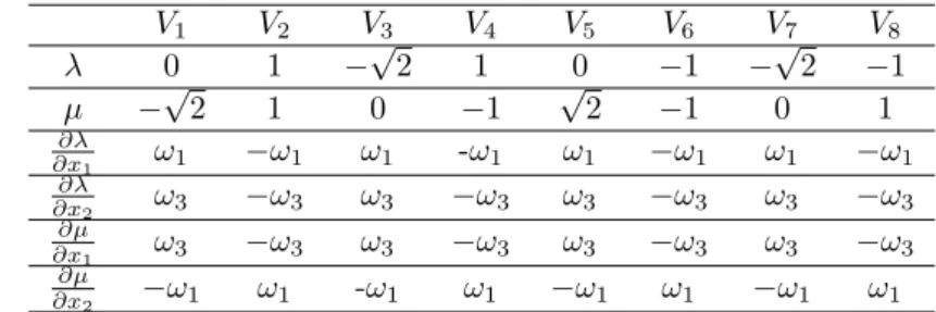
Now, using (3.13), (3.16) and (3.17), we can list the function values and gradients ofλandµat the verticesVi’s of the octagon Ω into Table 3.1.
V1 V2 V3 V4 V5 V6 V7 V8 λ 0 1 −√2 1 0 −1 −√2 −1 µ −√2 1 0 −1 √2 −1 0 1 ∂λ ∂x1 ω1 −ω1 ω1 -ω1 ω1 −ω1 ω1 −ω1 ∂λ ∂x2 ω3 −ω3 ω3 −ω3 ω3 −ω3 ω3 −ω3 ∂µ ∂x1 ω3 −ω3 ω3 −ω3 ω3 −ω3 ω3 −ω3 ∂µ ∂x2 −ω1 ω1 -ω1 ω1 −ω1 ω1 −ω1 ω1
Table 3.1. Function values and gradients of λandµatVi’s
By using the special choice of Ω and observing the values in Table 3.1, we can ask the functionsλandµto have the properties
µ(x1, x2) =λ(−x2, x1) (3.19) and
λ(x1, x2) =−λ(−x1,−x2) (3.20) for all (x1, x2) ∈ R2. Further, by (3.20), we could think of constructing the functionλby a polynomial function with only odd orders.
In the next subsection, we will construct a simple function that only meets the requirements (a) and (c) that are described in the first section. In§3.4, we construct a complicated function that can meet all the requirements (a), (b) and (c).
3.3
A Simple Function that Meets (a) and (c)
If we ignore the convexity requirement (b) of the line search function, we can construct a relatively simple functionλ(x1, x2) to meet the interpolation condi-tions listed in Table 3.1 and the functionµ(x1, x2) is then given by (3.19).
In fact, we can check that the following function λf(x1, x2)=(15−21 2 √ 2)x5 1+ (6− 9 2 √ 2)(x4 1x2+ 2x21x32) + (−15 + 10 √ 2)x3 1 +(−1 +√2)(6x21x2+x32) + (154 −15 8 √ 2)x1−9 8 √ 2x2.
has values of 0, 1, −√2, 1 at vertices V1, V2, V3, V4, respectively, and zero derivatives at all the verticesVi’s. Further, we can check the following function
λg(x1, x2) =−3−2 √ 2 4 (2x 2 1−1)[2x 2 1−(3 + 2 √ 2)]x2
has zero function values at all the verticesVi’s, but could be used to interpolate the derivatives ofλ(x1, x2) at Vi’s. Consequently, we know that
¯
λ(x1, x2) =λf(x1, x2) +ω1λg(x1, x2) +ω3λg(−x2, x1) (3.21) meets all the interpolation conditions required byλ(x1, x2) in Table 3.1. Conse-quently, we could say that for the function defined by (3.11), (3.21) and (3.19), the BFGS method with the Wolfe line search using the unit initial step does not converge.
Observing that
Ψi(α) =tΨi(α), Ψ0i(α) =tΨ0i(α) atα= 0,1,
we ideally wish there is the following relation between Ψi(α) and Ψi+1(α): Ψi+1(α) =tΨi(α), for allα≥0 (3.22) so that the neighboring line search functions only differ up to a constant mul-tiplier of t. However, the choice (3.21) of ¯λ(x1, x2) does not lead to (3.22). Nevertheless, we can propose the following compensation function
λc(x1, x2) =x1 x21+x22−(2 +√2)2 and define ˆ λ(x1, x2) = ¯λ(x1, x2) + ¯c1λc(x1, x2) + ¯c2λc(−x2, x1), (3.23) where ¯ c1 = (−39 + 15 √ 2)t−(2529−1756√2) 272 , ¯ c2 = (−65 + 8 √ 2)t+ (681−462√2) 272 .
In this case, the relation (3.22) will always hold and the corresponding line search function at the first iteration is
ˆ Ψ1(α) = 6 X i=0 ρiαi, (3.24) where ρ6 = (−3186 + 2233√2)t+ (3414−2398√2) 2 , ρ5 = (40347402−28052171 √ 2)t−(44367385−31014036) 9266 , ρ4 = (−18674096 + 12804379 √ 2)t+ (20961677−14552090√2) 4633 , ρ3 = (12350618−8366705 √ 2)t−(13736673−9508816√2) 9266 , ρ2 = (−211982 + 366273√2)t+ (40258−176758√2) 9266 , ρ1 = gT 1δ1= (−44 + 13 √ 2)t+ (40−18√2), ρ0 = f(x1) = (3954−4376 √ 2)t+ (18866−9563√2) 4633 .
To sum up at this stage, for the function (3.11) withλ(x1, x2) given in (3.21) or (3.23) andµ(x1, x2) =λ(−x2, x1), if the initial point isx1= (a1, b1, p1, q1)T (see (3.4), (3.8), (2.47) for their values) and if the initial matrix is H1 given by (2.58) and (2.59), then the BFGS method (1.2) and (1.5) with αk ≡ 1 will generate the iterations in (3.5) whose gradients are given by (2.4)-(2.5). Therefore the method will asymptotically cycle around the eight vertices of a regular octagon without approaching a stationary point or pushing f(xk) →
−∞.
3.4
A Complicated Function that Meets (a), (b) and (c)
To meet the requirement (b), this subsection gives a further compensation to the function ˆλ(x1, x2) in (3.23) such that each line search function Ψk(α) is strongly convex.
To this aim, we consider the straight line connectingx8j+i andx8j+i+1:
li(α) =x8j+i+αδ8j+i=
ai+α ηi bi+α ξi t8j(pi+α γi) t8j(q i+α τi) . (3.25)
By (3.12), the line search function at the (8j+i)-th iteration is
Ψ8j+i(α) =t8jλ(ai+α ηi, bi+α ξi) pi+α γi+µ(ai+α ηi, bi+α ξi) qi+α τi. (3.26)
To be such that each line search function is a strongly convex function that has the unique minimizerα= 1, we firstly construct Ψ1(α) as follows
Ψ1(α) =ζ1(α−1)38+ζ2(α−1)2+ζ3, (3.27) where ζ1 = (173256−38127 √ 2)t+ (−138064 + 48586√2) 166788 ≈1.5468E−1, ζ2 = (377472−359709√2)t+ (−712544 + 577958√2) 166788 ≈1.0405E−3, ζ3 = (−11344 + 6675 √ 2)t+ (42494−26967√2) 4633 ≈6.1270E−1.
Due to our special construction, we know from (3.3) and|t|<1 that the third and fourth components of {xk} tend to zero. This with the general function form (3.11) implies that the limit of f(xk) is f∗ = 0. So the above Ψ1 is constructed such that
Ψ1(0) =f(x1), Ψ1(1) =f(x2), Ψ01(0) =g T
1δ1, Ψ01(1) =g T
2δ1= 0, (3.28) where the values off(x1),f(x2) andgT
1δ1 are given in§3.1 and byf∗= 0. In addition, the positiveness ofζi’s implies that Ψ1 is strongly convex. Thus we see that Ψ1is a desired strongly convex function that takesα= 1 as the unique minimizer. A reason why we choose a polynomial (3.27) of degree 38 will be explained in the last section.
To utilize the function ˆλ(x1, x2) in (3.23), we firstly develop the following relation between (3.27) and (3.24),
Ψ1(α) = ˆΨ1(α) + 4 X i=0 α(α−1)4i+2 7 X j=0 σ8i+jαj, (3.29)
whereσi = 0 (i= 39, . . . ,35) and
σ34=ζ1, σ33=−20ζ1, σ32= 190ζ1, σ31=−1140ζ1, σ30= 9405ζ1, σ29=−41724ζ1, σ28= 134406ζ1, σ27=−346104ζ1, σ26= 735471ζ1, σ25=−1307504ζ1, σ24= 1961256ζ1, σ23=−2496144ζ1, σ22= 12688732ζ1, σ21=−28289632ζ1, σ20= 38155344ζ1, σ19=−37442160ζ1, σ18= 30421755ζ1, σ17=−21474180ζ1, σ16= 13123110ζ1; σ15=−6906900ζ1, σ14= 30735705ζ1, σ13=−55057860ζ1, σ12= 51389130ζ1, σ11=−28048800ζ1, σ10= 10518300ζ1, σ9=−3365856ζ1, σ8= 906192ζ1, σ7=−201376ζ1, σ6= 841464ζ1, σ5=−1357056ζ1, σ4= 1041600ζ1, σ3=−376992ζ1, σ2= 58905ζ1−ρ6, σ1=−7140ζ1−ρ5+ 4ρ6, σ0= 630ζ1−ρ4+ 3ρ5−6ρ6.
Secondly, noting that the following relations hold for alli≥1, ai+1+α ηi+1 bi+1+α ξi+1 =R1 ai+α ηi bi+α ξi , pi+1+α γi+1 qi+1+α τi+1 =t R2 pi+α γi qi+α τi , we look for some element functionsφ(x1, x2) that satisfy for all (x1, x2)∈ R2,
φ(¯x1,x¯2) φ(−x¯2,x¯1) =R2 φ(x1, x2) φ(−x2, x1) , where ¯ x1 ¯ x2 =R1 x1 x2 . (3.30) There are a lot of possibilities for the choice of φ(x1, x2). The following are some of them required in this paper.
φ1(x1, x2) =x3
1−3x1x22, φ3(x1, x2) =x13x22−x1x42, φ5(x1, x2) =x51−5x31x22, φ7(x1, x2) =x51x22−x1x62.
(3.31)
We takeφ1as an illustrative example. In fact, for any (x1, x2)∈R2, (¯x1,x¯2)T = R1(x1, x2)T means that ¯ x1= √ 2 2 (x1−x2), x¯2= √ 2 2 (x1+x2). Therefore we have that
φ(¯x1,x¯2) φ(−x¯2,x¯1) = ¯ x1(¯x21−3¯x22) ¯ x2(3¯x21−x¯22) = √ 2 4 (x1−x2)((x1−x2) 2−3(x1+x2)2) √ 2 4 (x1+x2)(3(x1−x2) 2−(x1+x2)2) ! = − √ 2 2 (x1−x2)(x 2 1+ 4x1x2+x22) √ 2 2 (x1+x2)(x 2 1−4x1x2+x22) ! = − √ 2 2 [(x 3 1−3x1x22) + (3x21x2−x32)] √ 2 2 [(x 3 1−3x1x22)−(3x21x2−x32)] ! = − √ 2 2 [φ(x1, x2) +φ(−x2, x1)] √ 2 2 [φ(x1, x2)−φ(−x2, x1)] ! = R2 φ(x1, x2) φ(−x2, x1) .
So φ1(x1, x2) is a desired element function. Similarly, we can check that the otherφi’s in (3.31) have the same property. In addition, it is easy to see that if φ(x1, x2) has the property (3.30), then φ(−x2, x1) keeps the same property. So we also consider the following element function
φ2i(x1, x2) =φ2i−1(−x2, x1), fori= 1,2,3.
Thirdly, we consider the linear combination ofφi(i= 1, . . . ,8) and define
λφ(x1, x2) = 8
X
i=1
Meanwhile, we defineµφ(x1, x2) =λφ(−x2, x1). For any vectorκ= (κ0, . . . κ7)T in R8, we are going to claim that there exists a unique solution of ν := (ν1, . . . , ν8)T such that the related functionsλφ andµφ satisfy
λφ(a1+α η1, b1+α ξ1) p1+α γ1 +µφ(a1+α η1, b1+α ξ1) q1+α τ1 = 7 X i=0 κiαi. (3.33) In fact, it is easy to see that the above relation leads to a linear system ofν:
Wν = κ. (3.34)
Direct calculations show that
W = W1+W2√2t+ (W3+W4√2, (3.35) whereWi(i= 1, . . . ,4) are given in the Appendix.
By further calculations, we know that Det(W) = ¯c3+ ¯c4 √ 2 t+ ¯c5+ ¯c6 √ 2 6 = 0, where ¯ c3 = −27257845112258321913344128791249391071037800448, ¯ c4 = −19354403625460153870213404828142913697757847552, ¯ c5 = 21709509966956378375726991567920438736281239552, ¯ c6 = 15449462608361267330121261246186521297040162816. HenceW is nonsingular and (3.34) is a nonsingular linear system. Therefore for any vectorκ∈ R8, there exists a uniqueν or λ
φ such that the relation (3.33) holds. For convenience, we denote suchλφ byλφ,κ.
Denoting the following vectors related to the coefficients {σi;i= 0, . . . ,39} in (3.29),
κi= (σ8i, . . . , σ8i+7)T, i= 0, . . . ,4,
and noticing that for any pointx= (x1, x2, x3, x4)T in the lineli(α) (iany), x21+x22−(2 +
√
2) = 2α(α−1), (3.36) we can finally present the desired function ofλ:
λ(x1, x2) = ˆλ(x1, x2) + 4 X i=0 " x21+x22−(2 +√2) 2 #4i+2 λφ,κi(x1, x2). (3.37)
Thus by the choice of ˆλ(x1, x2) in (3.23), the relation (3.36), the definitions of κi and λφ,κi and the relation (3.29), we know that the function (3.11) with
λ(x1, x2) given in (3.37) and µ(x1, x2) = λ(−x2, x1) not only satisfies those necessary interpolation conditions but gives the line search function
Ψi+1(α) =tiΨ1(α), for anyi≥0, (3.38) where Ψ1(α) is given by (3.27).
Since the polynomial functionλ(x1, x2) in (3.37) is of order 43, we see that the final objective function in (3.11) is a polynomial of order 44 and hence is infinitely times differentiable. The line search functions, which are given by (3.38) and (3.27), is strongly convex and has the unit stepsize as its unique minimizer. The requirement (b) is then satisfied.
In summary, for the function (3.11) with λ(x1, x2) given in (3.37) and µ(x1, x2) =λ(−x2, x1), if the initial point isx1 = (a1, b1, p1, q1)T (see (3.4), (3.8), (2.47) for their values) and if the initial matrix isH1 given by (2.58) and (2.59), then the BFGS method (1.2) and (1.5) withαk≡1 will generate the it-erations in (3.5) whose gradients are given by (2.4)-(2.5). Therefore the method will asymptotically cycle around the eight vertices of a regular octagon without approaching a stationary point or pushingf(xk)→ −∞.This counter-example is perfect in the sense that all the requirements (a), (b) and (c) are satisfied.
4
Concluding Remarks
No matter whether the simple example(s) in§3.3 or the complicated example in
§3.4, we can see that the BFGS method with unit stepsizes produces the same iterations{xk}and simultaneously, their objective functions provide the same gradients{gk}. As analyzed in§3.1, the unit stepsize is acceptable by the Wolfe line search, the Armijo line search or the Goldstein line search. If we do not impose the convexity on the line search function Ψk(α) for all k, it is possible for us to construct a relatively simple polynomial example shown in§3.3. The examples have the dimension 4, but can be used to show that the BFGS method may also fail for general functions whenn≥5 since four-dimensional functions can be regarded as special cases of higher-dimensional functions. In the case that n≥5, we can just take the same objective function and ask the starting pointx1to have zero components except the first four. Then for allk, the first four components ofxk remain the same as in the example and its components from the fifth will be always zero.
The counter-example in§3.4 is perfect in stepsize choices and function prop-erties. However, it is still not perfect in the sense that the objective function is very complicated with large numbers and some coefficients are expressed by nonsingular linear systems. Here we provide the reason why a polynomial (3.27) of degree 38 is used to guarantee the strong convexity of Ψ1(α). Equivalently, the problem of finding a strictly convex polynomial that satisfies (3.28) (in this case Ψ001(α) is nonnegative for all α ∈ R) can be transferred to the feasibility problem of some semi-definite program (SDP). This is because, by Shor [25], if n= 1, a polynomial is nonnegative if and only if it can be written into a sum of squares (s.o.s.); further, by Lasserre [12], for an any-dimensional polynomial,
it has the form of s.o.s. if and only if the coefficient matrix, which is formed when lifting the outer product of the vector of monomials and its transpose into the matrix variable, is semi-definite. The other interpolation conditions can be treated as linear constraints. However, even when we chose some relatively high numbers for the order of the desired polynomial, our numerical calcula-tions showed that the corresponding SDP feasibility problems have no solution. This is not expected since there are many freedoms in these polynomials, but there are only four interpolation conditions in (3.28). Instead, we considered the following simple form for Ψ1(α) with variable but evenp.
Ψ1(α) = ¯c1(α−1)p+ ¯c2(α−1)2+ζ3, (4.1) where ¯c1and ¯c2are parameters andζ3is the same constant in (3.27). With this form, it can be deduced from (3.28),f∗= 0 and the calculations in§3.1 that
1 p ≤ Ψ1(1)−Ψ1(0) Ψ0 1(0) = f(x2)−f(x1) gT 1δ1 ≈2.6483E−02. (4.2) Since the reciprocal of 2.6483E−02 is about 37.76, we choosepto be the least even integer, that is 38, to meet the condition (4.2).
In spite of the existence of large numbers, we have observed the cycle exactly predicted by the simple example in §3.3 (with the function ˆλ(x1, x2) given by (3.23)), thanks to the powerful symbolic computation software MAPLE. With such software, it is also possible to observe how numerical errors affect the ex-ample. When the machine error is set to 10−64(this is possible in MAPLE), we found that the cycle can go on for ten rounds and during the rounds, the itera-tions really tend to the eight vertices of the octagon according to the predicted way. Influenced by the numerical errors, however, the iterations jump out from the cycle during the eleventh round.
For quasi-Newton methods, there is global convergence if the norms of the matrixHk and its inverse are uniformly bounded for all k, in which case the angle between the quasi-Newton direction and the negative gradient must be uniformly less than some angle strictly less thanπ/2. For our examples, with the help of (2.2) and (2.57), we can see that the matrices{H8j+1;j= 1,2, . . .} satisfy the relation (2.24). Consequently, we have for allj≥1,
H8j+1= diag(t−4jE2, t4jE2)H1diag(t−4jE2, t4jE2). (4.3) By comparingH8j+1and the right matrices in (4.3) but with the middle matrix H1 replaced byλmin(H1)E4 andλmax(H1)E4, respectively, we can show that
λmax(H8j+1)≥t−8jλmin(H1), λmin(H8j+1)≤t8jλmax(H1), (4.4) whereλmax(·) and λmin(· · ·) mean the largest and smallest eigenvalues of the matrix. Since t is the decay parameter that lies in the interval (0,1), the relation (4.4) implies that both||H8j+1||2 and ||H8j+1−1 ||2 tend to infinity at an exponential rate. This analysis is also valid for{H8j+i;j= 1,2, . . .}with other i’s.
The number of the cyclic points in the above example(s) is eight due to the special choices ofθ1 andθ2 in (2.3). This number of eight could be decreased to seven since if
θ1=2
7π, θ2= 4 7π,
the consistent conditions (2.33)-(2.36) also allow a nonzero solution oft, whose numerical value is approximately 0.8642. However, it is difficult to obtain its analytic expression. In addition, we found that the system (2.33)-(2.36) has no solution oft in (−1,1) for
θ1= i
6π, θ2= j
6π, where i, j is any integer in [1,6], which implies that the number of cyclic points cannot be decreased to six.
As mentioned in§1, if the stepsize is chosen to be the first local minimizer along the line; namely, by (1.9), Powell [22] established the global convergence of the BFGS method for general differentiable functions whenn = 2. We ar-gued there that it is difficult to extend Powell’s result to the case that n= 3. Considerable attentions have also been drawn to the construction of a three-dimensional example (see also Section 5 of Powell [22]). This construction is al-most successful, but remains one condition always not satisfied. It is not known yet whether the BFGS method with the specific line search (1.9) converges for three-dimensional general differentiable functions.
Another direction of research is how to present a suitable modification of the BFGS algorithm, with which global convergence can be established for general nonconvex functions. A typical work of this kind is Li and Fukushima [13].
Acknowledgements. This work is initiated while the author was visiting Cambridge from July to October in 1997. He is very grateful to Professor Michael Powell and Professor Ya-xiang Yuan for their financial supports of his visit and consistent encouragements in many years. He also thanks the two anonymous referees very much for their useful suggestions and comments on this paper.
References
[1] R. H. Byrd, J. Nocedal, and Y. X. Yuan, Global convergence of a class of quasi-Newton methods on convex problems,SIAM J. Numer. Anal., 24 (1987), pp. 1171–1190.
[2] C. G. Broyden,The convergence of a class of double rank minimization algorithms: 2. The new algorithm,J. Inst. Math. Appl., 6 (1970), pp. 222– 231.
[3] Y. H. Dai,Convergence properties of the BFGS algorithm, SIAM Journal on Optimization, 13:3 (2002), pp. 693-701.
[4] W. C. Davidon,Variable metric methods for minimization,SIAM J. Op-tim., 1 (1991), pp. 1–17.
[5] J. E. Dennis and J. J. Mor´e, Quasi-Newton method, motivation and theory, SIAM Review 19 (1977), pp. 46-89.
[6] L. C. W. Dixon, Variable metric algorithms: Necessary and sufficient conditions for identical behavior of nonquadratic functions,J. Optim. The-ory Appl., 10 (1972), pp. 34–40.
[7] R. Fletcher, A new approach to variable metric algorithms, Computer J., 13 (1970), pp. 317–322.
[8] R. Fletcher,An Overview of Unconstrained Optimization, in Algorithms for Continuous Optimization: The state of Art, E. Spedicato ed., Kluwer Academic Publishers, Dordrecht/Boston/London, 1994, pp. 109-143. [9] R. Fletcher and M. J. D. Powell, A rapidly convergent descent
method for minimization,Comput. J., 6 (1963), pp. 163–168.
[10] D. Goldfarb,A family of variable metric methods derived by variational means,Math. Comp., 24 (1970), pp. 23–26.
[11] M. R. Hestenes and E. Stiefel,Method of conjugate gradient for solv-ing linear system,J. Res. Nat. Bur. Standards, 49 (1952), pp. 409–436. [12] J.B.Lasserre, Global optimization with polynomials and the problem of
moments, SIAM Journal on Optimization, 11:3 (2001), pp. 796–817. [13] D. H. Li and M. Fukushima, On the global convergence of the BFGS
method for nonconvex unconstrained optimization problems, SIAM Journal on Optimization, 11 (2001), pp. 1054–1064.
[14] W. F.Mascarenhas, The BFGS algorithm with exact line searches fails for nonconvex functions, Mathematical Programming, 99:1 (2004), pp. 49– 61.
[15] J. Nocedal, Theory of algorithms for unconstrained optimization, Acta Numer., 1 (1992), pp. 199–242.
[16] E. Polak and G. Ribi`ere, Note sur la convergence de methodes de di-rections conjugu´ees,Rev. Franccaise Informat. Recherche Op´erationelle, 16 (1969), pp. 35–43.
[17] B. T. Polyak,The conjugate gradient method in extremal problems,USSR Comp. Math. and Math. Phys., 9 (1969), pp. 94–112.
[18] M. J. D. Powell, On the convergence of the variable metric algorithm, J. Inst. Math. Appl., 7 (1971), pp. 21–36.
[19] M. J. D. Powell, Quadratic termination properties of minimization al-gorithm, Part I and PartII, J. Inst. Math. Appl., 10 (1972), pp. 333–357. [20] M. J. D. Powell,Some global convergence properties of a variable metric algorithm for minimization without exact line searches, in Nonlinear Pro-gramming, SIAM-AMS Proceedings Vol. IX, R. W. Cottle and C. E. Lemke, eds., SIAM, Philadelphia, PA, 1976, pp. 53–72.
[21] M. J. D. Powell,Nonconvex minimization calculations and the conjugate gradient method,in Numerical Analysis, D. F. Griffiths, ed., Lecture Notes in Math. 1066, Springer-Verlag, Berlin, 1984, pp. 122–141.
[22] M. J. D. Powell, On the convergence of the DFP algorithm for uncon-strained optimization when there are only two variables, Math. Program. Ser. B, 87 (2000), pp. 281–301.
[23] D. Pu and W. Yu,On the convergence property of DFP algorithm,Ann. Oper. Res., 24 (1990), pp. 175–184.
[24] D. F. Shanno,Conditioning of quasi-Newton methods for function mini-mization,Math. Comp., 24 (1970), pp. 647–650.
[25] N. Z. Shor,Quadratic optimization problems, Soviet J. Comput. Systems Sci., 25 (1987), pp. 1–11.
[26] W. Y. Sun and Y. X. Yuan, Optimization Theory and Methods: Non-linear Programming, Springer, New York, 2006.
[27] P. Wolfe, Convergence conditions for ascent methods, SIAM Rev., 11 (1969), pp. 226–235.
[28] Y. X. Yuan, Numerical Methods for Nonlinear Programming, Shanghai Scientific and Technical Publishers, Shanghai, 1993 (in Chinese).
Appendix. The matriciesWi(i= 1, . . . ,4) in the relation (3.35) are given in the following sequentially.
−62168 −15364 −50467 −19383 −50467 −19383 −170784 −69850 325732 7844 164094 202386 412766 −356414 617846 774894 −993360 196008 −4160 −201438 −2561400 1153290 −149012 −1366496 921688 0 3698860 −613452 −114596 463300 −869492 −653360 −296512 −333576 −407704 890484 −2569920 −2316500 −168300 3018560 0 0 296512 −333576 1546864 1667880 1142176 −3712088 0 0 0 0 −593024 −667152 −1408432 2448120 0 0 0 0 0 0 593024 −667152
−38766 −23402 −34925 −15542 −34925 −15542 −120317 −50467 64624 102164 94362 165678 249426 −238058 422668 564826 94320 101688 144215 −260041 −1444145 928375 25696 −1083960 −563244 −500364 −488404 −117052 1201020 −648620 −1191110 3882 315044 315044 213118 206782 1009350 880270 1283770 1018070 0 0 −18532 −18532 −1700980 −1575220 −1143596 −1018308 0 0 0 0 630088 630088 463300 450628 0 0 0 0 0 0 −37064 −37064 66580 −22806 48866.5 −2955.5 48866.5 −2955.5 162176 −419 −305222 82838 −149974 −138071 −193910 377473 −543381 −565187 1072146 −156966 2300535 8467 135353 −905635 75885 1149501 −1085404 −74128 43774 654056 −3792690 −741280 700702 782668 333576 333576 444768 −845924 3017860 2409160 429750 −2916010 0 0 −296512 296512 −1948424 −1704944 −1357948 3555920 0 0 0 0 667152 667152 1482560 −2284872 0 0 0 0 0 0 −593024 593024 31153 16895 32221.5 2746 32221.5 2746 113309.5 2536.5 49886 −124014 −72850 −147478 −49206 243454 −360117 −438519 −280980 12822 −169365 304282 980815 −762350 −120120 1044365 632088 444768 −554550 465018 10702 509630 1166840 −228060 −315044 −315044 −194586 −93378 −1538890 −880270 −1213170 −445520 0 0 18532 −18532 1838668 1575220 1059760 467608 0 0 0 0 −630088 −630088 −426236 −149692 0 0 0 0 0 0 37064 −37064