Hydrol. Process.(in press)
Published online in Wiley InterScience
(www.interscience.wiley.com) DOI: 10.1002/hyp.6555
Impact of time-scale of the calibration objective function on
the performance of watershed models
K. P. Sudheer,
1I. Chaubey,
2* V. Garg
1and Kati W. Migliaccio
31Department of Biological and Agricultural Engineering, University of Arkansas, Fayetteville, AR 72701, USA
2Department of Agricultural and Biological Engineering and Department of Earth and Atmospheric Sciences, Purdue University, West Lafayette, IN
47906, USA
3Agricultural and Biological Engineering Department, University of Florida Tropical Research and Education Center, 18905 SW 280 Street,
Homestead, FL 33031, USA
Abstract:
Many of the continuous watershed models perform all their computations on a daily time step, yet they are often calibrated at an annual or monthly time-scale that may not guarantee good simulation performance on a daily time step. The major objective of this paper is to evaluate the impact of the calibration time-scale on model predictive ability. This study considered the Soil and Water Assessment Tool for the analyses, and it has been calibrated at two time-scales, viz. monthly and daily for the War Eagle Creek watershed in the USA. The results demonstrate that the model’s performance at the smaller time-scale (such as daily) cannot be ensured by calibrating them at a larger time-scale (such as monthly). It is observed that, even though the calibrated model possesses satisfactory ‘goodness of fit’ statistics, the simulation residuals failed to confirm the assumption of their homoscedasticity and independence. The results imply that evaluation of models should be conducted considering their behavior in various aspects of simulation, such as predictive uncertainty, hydrograph characteristics, ability to preserve statistical properties of the historic flow series, etc. The study enlightens the scope for improving/developing effective autocalibration procedures at the daily time step for watershed models. Copyright2007 John Wiley & Sons, Ltd.
KEY WORDS model calibration; uncertainty; SWAT; rainfall-runoff
Received 22 April 2005; Accepted 7 June 2006
INTRODUCTION
Conceptual rainfall–runoff models are widely used for flood forecasting, water quality predictions, and for mak-ing watershed management decisions. Such models pro-vide an approximate, lumped description of the dominant subwatershed-scale processes that contribute to the over-all watershed-scale hydrologic response of the system (Boyle et al., 2000). There are a plethora of watershed models available to date that vary in degree of complex-ity (e.g. Thornthwaite and Mather, 1955; Crawford and Linsley, 1966; Xu and Singh, 1998). All these models describe, conceptually, land-based hydrological processes that are spatially averaged or lumped.
However, a major constraint for application of these conceptual models is the number of parameters that need to be estimated or defined so that the modelled response to rainfall closely simulates the actual behaviour of the watershed of interest. For example, the Sacramento Soil Moisture Accounting model (Burnash et al., 1973) is used by the National Weather Service for flood fore-casting throughout the USA. The model has 17 param-eters whose values must be specified. Although a few of these parameters might be estimated by relating them
* Correspondence to: I. Chaubey, Department of Agricultural and Biolog-ical Engineering and Department of Earth and Atmospheric Sciences, 225 South University Street, Purdue University, West Lafayette, IN 47906, USA. E-mail: [email protected]
to observable characteristics of the watershed, most are abstract conceptual representations of non-measurable watershed characteristics that must be estimated through a calibration process. The Soil and Water Assessment Tool (SWAT), developed by the United States Department of Agriculture (Arnold et al., 1998), is another conceptual model that is being widely employed for making water-shed flow and water quality response predictions as a function of land use, soil, management, and weather input data (Arnold and Fohrer, 2005). SWAT also has a number of parameters that need to be estimated through a calibra-tion procedure. Other commonly used conceptual models are the HEC-1 (US Army Corps of Engineers, 1990) and the Stanford Watershed Model (SWM; Crawford and Linsley, 1966). Although such models ignore the spa-tially distributed, time-varying, and stochastic properties of the hydrological processes, they attempt to incorpo-rate realistic representations of the major non-linearities inherent in the rainfall runoff process (Hsuet al., 1995). These models have been reported to be reliable in fore-casting the hydrograph characteristics, such as the rising limb, the time and the height of the peak, and volume of flow (Sorooshian, 1983); however, their implementation and calibration can typically present various difficulties (Duanet al., 1992). The calibration requires sophisticated mathematical tools (Sorooshian et al., 1993), significant amount of calibration data (Yapoet al., 1998), and some degree of expertise and experience with the model.
Model calibration involves the selection of values for the model parameters so that the model matches the behaviour of the watershed system as closely as possible. During the calibration of any conceptual model, literature values are generally used to assign initial parameter values based on the soil type, land use, or some other index, because of the dearth of field-measured parameter values. These initial estimates of parameter values are then adjusted during calibration to simulate the measured flow at the watershed outlet. Models developed in this manner have produced varying results in terms of simulating watershed runoff (Downer and Ogden, 2003). Typically, model parameters for gauged catchments are usually estimated by ordinary least squares, which involves solving the following minimization problem:
min sum of squaresDminD
n
tD1
[qt.obsqt.simxt;A]2
1
where qt.obs and qt.sim are the observed and simulated
flows respectively (the difference of which is the model residual errorεt),xt is a vector of inputs (such as rainfall and any exogenous variables such as evaporation, snow, etc.) andAis a parameter vector about which inference is sought. The use of Equation (1) as an objective function to be minimized for parameter estimation implies certain assumptions about the residuals εt (Clarke, 1973; Xu, 2001):
1. that εt have zero mean and constant variance ε2 (i.e.
EεtD0,Eε2tεDε2);
2. that theεtare mutually uncorrelated (i.e.Eεt, εtkD 08k6D0).
The above assumptions need to be tested for the residuals of the model. It is observed that most of the studies in hydrology do not report the verification of these hypotheses, though a visual inspection of predicted and measured hydrograph together with a ‘goodness of fit’, such as coefficient of determinationR2, are generally presented.
Yet another concern in model calibration is the tem-poral and spatial scale in which the simulations should be compared with the measured value of the variable. Although spatially distributed models demonstrate con-siderable skill in predicting flow at the watershed out-let, they do not illustrate that the models are accurately describing natural processes occurring at the sub-basin scale (Garget al., 2003). Whereas the temporal scale of comparison is not important for event-based conceptual models (such as HEC-1), the performance of continu-ous simulation models (such as SWAT or SWM) would be greatly affected by the time-scale of calibration. For example, the SWAT model, which simulates on a daily time step (Arnold and Fohrer, 2005), is generally cal-ibrated at the annual level (Neitsch et al., 2002a), and the parameters are fine-tuned by considering disaggre-gated time steps, e.g. monthly time steps. The mere
application of process-based models implies that actual processes are being correctly simulated. Assertions that such models actually mimic hydrologic processes even at a smaller time step than it has been calibrated for, and not merely reproduce observed flows by empirical rela-tionships, requires that independent measures be used to validate this claim. In most of the applications where models are calibrated at a higher (aggregated) time step, such as annual level or monthly level (e.g. Srinivasan and Arnold, 1994; Spruillet al., 2000), this is not reported.
The objective of this paper is to evaluate the effect of the calibration objective function time-scale on model performance and to demonstrate the importance of resid-ual statistical analysis in assessing the fitted model. For this purpose the SWAT model is calibrated to simulate the monthly flow at the watershed outlet for War Eagle Creek basin in Arkansas, USA. Although the purpose of our study is not to develop an algorithm for calibration of models at smaller time steps (such as daily), which is typically highly complex, the study examines the require-ment for such an algorithm.
THE MODEL AND DATA
Description of the SWAT model
We used the SWAT model as an example model to demonstrate the effect of time-scale of model calibration on output uncertainty. Since the basic hydrologic rou-tines used in the SWAT model to represent hydrologic cycle are also common in many of the currently avail-able continuous-simulation distributed-parameter water-shed models, we expect the results to be applicable to other models. We must emphasize that the objective of this study is not to critique the SWAT model’s capability itself; rather, we have used this as an example in this study.
SWAT is a watershed-scale operational or conceptual model that operates on a daily time step. The model pre-dicts watershed response variables, such as stream flow, sediment, nutrient, bacteria, and pesticide transport, as a function of soil, land use, management, and climate con-ditions (Arnold and Fohrer, 2005). Being a physically based distributed parameter model, SWAT considers both upland and stream processes that occur in a watershed. The upland processes include hydrology, erosion, cli-mate, soil temperature, plant growth, nutrients, pesticides, and land management. Stream processes considered by the model include water balance, routing, and sediment, nutrient, and pesticide dynamics. The model has been extensively applied in a number of watersheds in the USA and in other countries. Arnold and Fohrer (2005), Jayakrishnan et al. (2005), and White (2005) have pro-vided detailed overviews of model application in making watershed response predictions.
The SWAT model divides a watershed into smaller sub-watersheds, based on stream network, location of point source data, and stream gauges. Each subwatershed is further subdivided into smaller areas called hydrologic
response units (HRUs), which are considered to be hydro-logically homogeneous. The model calculations are per-formed on an HRU basis. Loadings of water, sediment, nutrients, and pesticides from each HRU to the stream channel, and subsequently through the channel network, are routed using a method described by Williams and Hann (1972). Details of model configuration, including procedures for calculation of various model outputs, are given in Neitschet al. (2002a).
The soil water balance is the primary consideration by the model in each HRU, which is represented as (Arnold
et al., 1998) SWtDSWt1C t iD1 RiQiETiPiQRi 2 where SW is the soil water content, i is the time t
(days) for the simulation period, and R, Q, ET, P, and QR are respectively the daily precipitation, runoff, evapotranspiration, percolation, and return flow. SWAT is a continuous-simulation model, i.e. model parameters used to predict watershed response variables are updated on a daily time-scale. This allows the model to capture the dynamic response of the study watershed.
The surface runoff is computed using one of the two approaches: (i) the Green and Ampt infiltration method or (ii) the Soil Conservation Service (SCS) curve number (CN) method. Application of the Green and Ampt infiltration method requires input data on rainfall and infiltration at an hourly rate. Because of this limitation, the SCS-CN method is the most commonly used method for runoff prediction. According to the SCS-CN method, runoff from an HRU is a function of daily precipitation, soil, and land-use characteristics, and can be computed as (Neitschet al., 2002b)
QD R0Ð2s
2
RC0Ð8s R >0Ð2s
QD0 R0Ð2s 3
where Q is daily runoff, R is daily rainfall, and s is the retention parameter. The value of sdepends on soil, land use, and antecedent moisture conditions and can be estimated as (Neitschet al., 2002b) sD254 100 CN 1 4
where CN is the curve number.
Peak runoff rate in the SWAT model is calculated using the modified rational equation or SCS TR 55 method (USDA, 1986). Arnoldet al. (1998) and Neitsch
et al. (2002b) have provided details on how the model calculates other hydrologic and water quality parameters. It is worth mentioning that the water balance is the driving force behind all other watershed calculations in SWAT and, therefore, must be accurately simulated to estimate movement of sediment, nutrients, and pesticides from a watershed. A number of reports are available that describe the use of the SWAT model in making flow predictions (refer to White and Chaubey (2005) for a
detailed description of SWAT applications). Also, since the model uses the daily flow values to calculate nutrient, sediment, pesticides, and other model outputs, it is very important that model-predicted watershed response data at the daily time-scale accurately mimic the actual watershed processes.
Description of the study watershed and data used
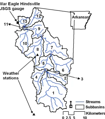
The data used in this study were obtained from War Eagle Creek watershed, having an area of 68 100 ha, located in northwest Arkansas, USA. The predominant land uses in the watershed are forest (63Ð7%) and pasture (35Ð6%). Nutrients and sediment sources include animal agriculture (poultry, swine, and cattle production), and point-source flow from a wastewater treatment plant (WWTP) from the city of Huntsville. Water quality of the War Eagle Creek is currently a concern, since it forms a tributary to Beaver Lake, a drinking-water reservoir for more than 300 000 people in northwest Arkansas, USA. Figure 1 shows the location of the watershed, stream network, subwatershed representation of the SWAT model, and location of the stream and weather gauges.
The data pertaining to the study area have been obtained from various sources. A 30 m digital elevation model (from the US Geological Survey), STATSGO soil data (US EPA, 2004), and 28Ð5 m use and land-cover data (from CAST (2002)) were used in the SWAT model. The watershed was divided into 13 subwater-sheds based on stream network characteristics within the watershed. It should be noted that the disaggregation of a watershed into subwatersheds is user defined and is done in the SWAT model to identify and rank subwater-sheds based on their runoff and water quality response.
Weather data (including daily minimum and maximum temperatures and rainfall) from two stations (Figure 1) were available for the study. Other meteorological data, such as solar radiation, were generated using a weather generator program available in the SWAT model. In addi-tion, point- and non-point-source data used in the model included WWTP effluent flow rate and concentration and animal manure and inorganic fertilizer application rates in the watershed. The meteorological data and the stream-flow data considered for the study were for a period of 4 years during 1999– 2002 on a daily time step.
METHODOLOGY
Model calibrations
Available data during the period 1999– 2000 were used for the SWAT model calibration, and the model was val-idated using the data for the period 2001– 2002. Since SWAT has a large number of parameters, a sensitivity analysis was first conducted to identify the set of param-eters that had the most influence on predicted flow, using the procedure described by James and Burges (1982). The relative sensitivity Sr was used to identify and rank all
the model parameters that influence predicted runoff:
SrD
O2O1
P2P1
P
O 5
where Owas the predicted output, Pwas the parameter value, and O2, O1 and P2, P1 represent š10% of the
initial output and parameter values respectively (James and Burges, 1982).
Parameters having the highest relative sensitivity to predicted runoff and total flow were curve number CN, soil evaporation compensation factor ESCO, available soil water capacity SOL AWC, average slope length SLSUBBSN, and moist bulk density of soil SOL BD. Detailed results of sensitivity analyses are presented else-where (White and Chaubey, 2005). These parameters were modified during the model calibration. Both cali-bration and validation were done at annual and monthly time steps.
The calibration of the model was achieved by the procedure suggested by Neitsch et al. (2002a), which is a sequential calibration process to achieve optimum calibration results for the SWAT model. The model was calibrated for flow predictions first at annual scale, followed by monthly and daily scales. The objective function used in annual calibration was minimization of the relative error RE between measured and predicted flow at the gauging location:
RE%Dqobsqsim qobs
ð100 6
where qobs m3 s1 is the measured annual flow and
qsim m3 s1 is the predicted annual flow. Once the
model was calibrated at the annual scale, the param-eters were fine-tuned on a monthly scale using the
Nash–Sutcliffe coefficient of model efficiencyRNS(Nash
and Sutcliffe, 1970) andR2:
RNSD1 n iD1 qobsqsim2 n iD1 qobsqcom2 7 R2 D n iD1
qobs.iqobsqsim.iqsim
n iD1 qobs.iqobs2 n iD1 qsim.iqsim2 0Ð5 2 8
whereqcomm3 s1is the average value of the observed
flow, and all other variables are as defined earlier. Note that, at annual and monthly time steps, the accumulated flows at these time steps are considered while evaluating the objective function.
Because the SWAT model is a distributed parameter model, many of the model parameters are unique at the HRU level. During the calibration process, each model parameter that was spatially variable was either increased or decreased to achieve the calibration objective function. However, the model is generally calibrated only at annual and monthly time-scales, as calibration at a daily time step becomes typically complex. In the current study, as the major objective was to evaluate the impact of the time-scale of the calibration objective function, the calibrated model parameters at the monthly time-scale (referred to as SWAT monthly calibrated (SMC) here-after) were further tuned by employing an autocalibration procedure at daily time steps (referred to as SWAT daily calibrated (SDC) hereafter). Note that the calibration at daily time steps requires complex optimization proce-dures and is computationally expensive. The objective function used for the automatic model calibration at the daily time-scale was maximization of R2 values defined
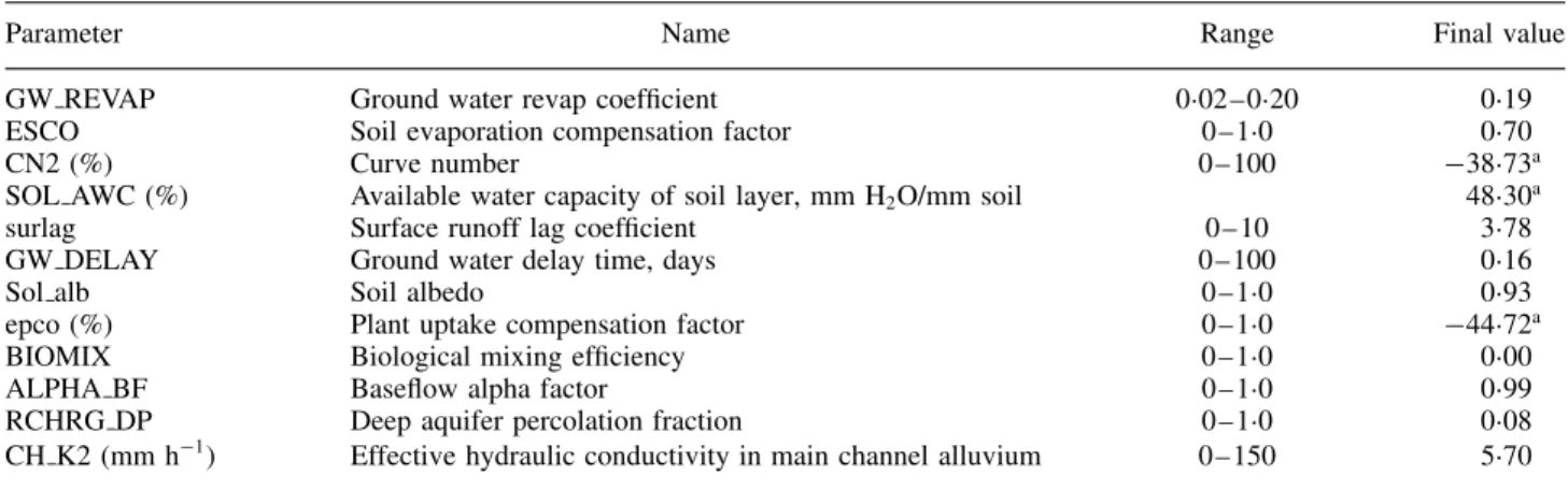
by Equation (8). A list of the parameters, their range of values and the final parameter values achieved after the autocalibration of the model are shown in Table I.
Performance evaluation of models
Similar to other distributed parameter models, SWAT also has limitations due to the non-identifiability of parameters, i.e. there more than one combination of parameter values exists that may result in the same model output. Qualitative assessments of the degree to which the model simulations match the observations are used to provide an evaluation of the model’s predictive abilities. Many of the principal measures that are used in the hydrological literature have been critically reviewed by Leagates and McCabe (1999). Still, there is diversity in the use of global goodness-of-fit statistics to determine how well the model forecasts the hydrograph. In the current study, a multicriteria assessment was performed in the absence of a single evaluation measure. The data from 2001– 2002 were used for model validation using
Table I. List of parameters, their range of possible values, and final calibrated values (after autocalibration at daily time-scale) for the SWAT model for War Eagle Creek, Arkansas
Parameter Name Range Final value
GW REVAP Ground water revap coefficient 0Ð02–0Ð20 0Ð19
ESCO Soil evaporation compensation factor 0–1Ð0 0Ð70
CN2 (%) Curve number 0–100 38Ð73a
SOL AWC (%) Available water capacity of soil layer, mm H2O/mm soil 48Ð30a
surlag Surface runoff lag coefficient 0– 10 3Ð78
GW DELAY Ground water delay time, days 0–100 0Ð16
Sol alb Soil albedo 0–1Ð0 0Ð93
epco (%) Plant uptake compensation factor 0–1Ð0 44Ð72a
BIOMIX Biological mixing efficiency 0–1Ð0 0Ð00
ALPHA BF Baseflow alpha factor 0–1Ð0 0Ð99
RCHRG DP Deep aquifer percolation fraction 0–1Ð0 0Ð08
CH K2 (mm h1) Effective hydraulic conductivity in main channel alluvium 0–150 5Ð70
aThese parameters are HRU specific, having a unique value for each HRU. The final value represents the percentage by which the default parameter value was changed for each HRU.
the criteria suggested by White and Chaubey (2005). In summary, according to White and Chaubey (2005), the model validation was considered successful if the evaluation statistics were similar in ranges to those determined during model calibration. The criteria that are employed are the root-mean-square error (RMSE) between the observed and simulated values, RNS, and
R2. In addition to these statistics, the model forecasts were checked for validity of the hypothesis upon which the calibration was based. The models are also evaluated for their predictive capabilities to preserve the summary statistics of the river flow series.
RESULTS, ANALYSES AND DISCUSSIONS
Performance of SWAT model at monthly time step
The goodness-of-fit statistics for the monthly flow simulations of War Eagle Creek basin by the SWAT model (SMC and SDC) are presented in Table II, from which it is apparent that the simulations are reasonably good. The high value of R2 during calibration (greater than 0Ð80 for both SMC and SDC) indicates a good agreement between the simulated and measured values of monthly flows. Note that reported values ofR2for various
watersheds during SWAT calibration range between 0Ð63 and 0Ð98 (computed at monthly time-scale; e.g. Arnold and Allen, 1996; Arnold et al., 1998; Srinivasan et al., 1998; Cotter et al., 2003). It is noted that the efficiency of the model, which is a measure of the model’s ability to predict values away from the mean, is satisfactory during calibration and validation (0Ð70– 0Ð81 during calibration and 0Ð41– 0Ð79 during validation for SMC). The RMSE is a measure of the residual variance and is indicative of the model’s ability to predict high flows. The low value of RMSE (3Ð98– 7Ð22 m3 s1 for SMC) implies
that the SWAT model is able to simulate the flows with reasonable accuracy. The values of the performance indices presented in the Table II were consistent during calibration and validation for the SMC model, except for
Table II. Goodness-of-fit statistics during calibration and valida-tion of the SWAT model calibrated for War Eagle Creek basin at a monthly time-scale (SMC) and a daily time-scale (SDC).
(Note: the statistics are computed at monthly time-scale) Calibration period Validation period
1999 2000 2001 2002 SMC R2 0Ð82 0Ð80 0Ð52 0Ð89 RNS 0Ð81 0Ð70 0Ð41 0Ð79 RMSE (m3 s1) 3Ð98 5Ð13 7Ð22 5Ð79 SDC R2 0Ð83 0Ð89 0Ð84 0Ð78 RNS 0Ð65 0Ð87 0Ð76 0Ð67 RMSE (m3 s1) 5Ð29 3Ð44 4Ð81 5Ð98
the year 2001, the reason for which needs to be explored further.
The performance statistics, computed for the SDC, are also presented in Table II. Note that the monthly cali-brated model (SMC) has been further fine-tuned at the daily time-scale using an autocalibration procedure; the fine-tuning autocalibration required ¾4 days of continu-ous computations that produced ¾4000 model runs. It is evident from Table II that improved SWAT predic-tions were obtained when the model was calibrated at the daily time-scale (see Table II for SDC). Higher R2
values were obtained for all years, except in 2002, when the model was calibrated at daily time-scale. The val-ues of RNS ranged from 0Ð65 to 0Ð87 and RMSE ranged
from 4Ð81 to 5Ð98 m3 s1 for daily calibration results. It is worth noting that the simulations during the year 2001 were improved in this case (an increase in efficiency from 0Ð41 to 0Ð76) in addition to improvement in other indices of model performance.
A plot of the simulated and measured flow values dur-ing calibration and validation years for SWAT models (SMC and SDC) is presented in Figure 2 for compari-son. From Figure 2, it is observed that the SWAT sim-ulated flows clearly follow the trend and variations in
Figure 2. Comparison of SWAT simulated and measured monthly flow for monthly time-scale calibration (SMC) and daily time-scale calibration (SDC)
Table III. Summary statistics (of monthly flow) of SWAT simulations calibrated at a monthly time-scale (SMC) and a daily time-scale (SDC) for War Eagle Creek basin
Calibration period Validation period
1999 2000 2001 2002
Obs. SMC SDC Obs. SMC SDC Obs. SMC SDC Obs. SMC SDC
Mean (m3 s1) 10Ð95 11Ð63 7Ð82 5Ð88 8Ð62 7Ð30 6Ð93 9Ð94 8Ð09 10Ð35 12Ð97 12Ð65
Standard deviation 9Ð38 7Ð56 6Ð39 9Ð79 9Ð76 9Ð92 10Ð28 6Ð99 6Ð78 13Ð00 9Ð12 7Ð99 Skewness coefficient 0Ð24 0Ð26 0Ð12 3Ð12 2Ð12 2Ð11 2Ð05 0Ð99 1Ð02 1Ð82 1Ð05 0Ð50
the observed flow records. It should be noted that the flow from War Eagle Creek basin during the months of August to November is relatively low compared with other months of the year, and the SWAT model is able to mimic these variations reasonably well, though SMC is consistently overpredicting the low flows. Similar model results have been reported by other researchers, where SWAT was found to overestimate low flow predictions (e.g. Boschet al., 2004; Chuet al., 2004). Model simu-lations significantly improved when calibrated on a daily time-scale (SDC) by more accurately predicting the high flows and low flows. Assessment of the potential of the SWAT model to preserve the statistical properties of the
historic flow records reveals that the first two statistical moments (i.e. mean and standard deviation) were repro-duced reasonably well by the model in both cases (see Table III).
Considering the above-discussed goodness-of-fit statis-tics and the summary statisstatis-tics, it is generally rea-sonable to conclude that the SWAT simulations cal-ibrated at a monthly time step are reasonably good, and the calibrated model may be employed for further analysis. However, the model has been calibrated with the objective to minimize the sum square of deviation between the observed and simulated flow values. Con-sequently, the above-considered goodness-of-fit statistics
Figure 3. Plot of residuals versus SWAT simulated monthly river flow for War Eagle Creek: (a) model calibrated at a monthly time-scale (SMC); (b) model calibrated at a daily time-scale (SDC)
Figure 4. Autocorrelation of residual from the SWAT model monthly simulations of War Eagle Creek (the dotted line indicatesš95% confidence level) for SWAT calibrated at a monthly time-scale (SMC) and SWAT calibrated at a daily time-scale (SDC)
would certainly suggest good performance for the model, as all the statistics are derived from the deviation between observed and simulated flow. Therefore, in order to test the robustness of the model, it is important to evaluate the model using some other performance indices. Accord-ingly, the residuals from the model simulations have been further analysed for verifying the basic assumptions dis-cussed earlier.
Figure 3 depicts the residuals plotted against the SWAT model simulated monthly flows for the calibration and validation periods (for both SMC and SDC). It is evident from Figure 3 that the SMC model predictions have a systematic bias in simulating the lower values of
runoff. Further, we observed that the residuals’ variability increases with increasing runoff in the case of the SMC model. This observation suggested that the assumption of constant error variance (homoscedasticity) was violated for the model calibrated at a monthly time step. However, the assumption of homoscedasticity was reasonably valid for the model calibrated at a daily time step (see Figure 3 for SDC); there was evidence that model predictions could be improved.
The residual autocorrelations together with the 95% confidence intervals are plotted in Figure 4 for both the SMC and SDC models. Residuals did not have a sig-nificant correlation (except at lag 1 during the validation
period for SMC). This implies that the hypothesis of inde-pendence of residuals for the SMC model was fulfilled in the simulations. This observation was also true in the case of the model calibrated at a daily time-scale. How-ever, it must be noted that the decay of autocorrelation was systematic for SMC model.
The foregoing discussions illustrate that a judgment on the model performance purely based on performance indices (such as RMSE,R2, etc.) may be misleading (i.e. they do not give any information about the homoscedas-ticity and independence of residuals) and that model per-formance benefits from being evaluated using a number of evaluation measures.
Performance of SWAT model at daily time step
As stated earlier, the SWAT model has generally been calibrated at monthly time-scales, whereas the model performs all of its calculations on a daily time step. Hence, the model performance at the smaller time-scale also needs evaluation before it can be further employed for making management decisions. The SWAT model simulated daily flows and the observed flows
are presented in a scatter diagram in Figure 5 for both the SMC and SDC models. SMC simulations were not satisfactory and did not coincide with measured values. Note that the R2 value for the SMC model was only 0Ð36 during the calibration period (1999– 2000) and 0Ð56 during the validation period (2001– 2002). A reduced scatter plot for the SDC model clearly illustrates a reasonably good simulation, with anR2value for the SDC
that was greater than that for the SMC.
The goodness-of-fit statistics were computed on daily time step (Table IV). The results indicate that SMC model efficiency values are often negative (except for 2002), which is indicative of highly biased model simu-lations. The RMSE values for the SMC model are high compared with the observed mean values for these years (cf. Table IV with Table III). On the contrary, the perfor-mance indices for the SDC model (see Table IV) were realistic (positive efficiency values) and were better than the monthly calibrated model. The R2 for the daily
sim-ulations ranged from 0Ð36 to 0Ð81, and R2 for the SMC
was between 0Ð28 and 0Ð63. An improvement of 39% in RMSE was observed for the SDC model compared
Figure 5. Scatter plot of daily values of SWAT simulated and observed flow for War Eagle Creek for model calibrated at a monthly time-scale (SMC) and model calibrated at a daily time-scale (SDC)
Table IV. Goodness-of-fit statistics during calibration and valida-tion of the SWAT model calibrated for War Eagle Creek basin at a monthly time-scale (SMC) and a daily time-scale (SDC).
(Note: the statistics are computed at daily time-scale) Calibration period Validation period
1999 2000 2001 2002 SMC R2 0Ð28 0Ð46 0Ð41 0Ð63 RNS 0Ð33 0Ð35 0Ð07 0Ð47 RMSE (m3 s1) 22Ð79 22Ð14 22Ð25 25Ð91 SDC R2 0Ð36 0Ð81 0Ð73 0Ð44 RNS 0Ð33 0Ð80 0Ð68 0Ð37 RMSE (m3 s1) 16Ð14 8Ð3 12Ð09 20Ð47
with the SMC model. This improved optimization of the model after autocalibration is in agreement with many reported studies.
The summary statistics (standard deviation and skew-ness with observed counterparts) of the daily flow series simulated by the model are depicted in Figure 6. The results from the SMC model indicate that the variance in the flow is not preserved, but that the skewness of the data is. In addition, the SDC model is able to maintain the variance better than the SMC model (Figure 6). In the case of model calibration on a monthly time-scale, the preservation of mean and skewness of the flow series indicates that the SWAT model is able to capture the non-linear features of the rainfall runoff process and the local patterns, but fails to represent the dynamic nature of the flow series effectively that was explained by the variance of the time-series. An examination of homoscedasticity and independence of the residuals at the daily time step suggests that the SWAT models calibrated on a monthly time-scale result in simulations where the daily predic-tions are not valid. However, the performance of the model calibrated on a daily time-scale based on these measures (homoscedasticity and independence of residu-als) is satisfactory. The results are not presented herein for brevity.
The results indicate that model simulations calibrated on a daily time-scale (SDC) significantly improve the
model calibrated on the monthly time-scale (SMC). The results indicate that the good model performance at an aggregated time-scale (e.g. monthly scale) is ensured by calibrating them at a disaggregated time-scale (e.g. daily scale).
REMARKS
It should be noted that, irrespective of the time-scale of calibration, the SWAT model computations were made on a daily basis at the HRU levels, and the total watershed runoff was estimated by routing the flows from individual HRUs. Hence, any uncertainty in the model simulations implies that the model is not accurately representing the runoff process at the scale of HRU levels. This claim was not substantiated, given the typical lack of data other than the stream flow at the watershed outlet. Moreover, when the model was calibrated at aggregated time steps, the model parameters were assigned values by comparing the accumulated monthly and annual flow values, which in turn neutralizes the errors at the daily time-scale. Further, linking error diagnostics with specific model deficiencies would require an in-depth examination of the model used in this illustration. The goal of this paper was to examine the impact of time-scale of calibration objective function on the model performance, not to diagnose the model itself.
Most of the studies that have used the SWAT model did not report the model’s performance at the daily time-scale, whereas all of them have been calibrated at the annual and/or monthly scales (see White and Chaubey (2005) for a compilation of SWAT model application results). Although this may be attributed to the requirement of complex optimization procedures for calibrating a number of model parameters at a daily time step, the results from this study clearly illustrate that the model’s performance at the smaller time-scale cannot be ensured by calibrating the model at a larger time-scale. Our results suggest the need for a simple calibration procedure for watershed models that can be easily implemented for a daily time step.
Figure 6. Plot of standard deviation and skewness of SWAT simulated daily flow for model calibrated over a monthly time-scale (SMC) and model calibrated over a daily time-scale (SDC)
SUMMARY AND CONLUSIONS
We have discussed the simulation of watershed runoff in hydrologic models in terms of their calibration. The objective of this paper was to evaluate the effect of time-scale of the calibration objective function on the model performance at disaggregated time levels. The results imply that evaluation of models based on any single overall statistic computed between the simulated and observed values, which aggregate the model perfor-mance over a large range of hydrological behaviour, does not ensure a good model performance. Furthermore, one should be careful not to arrive at erroneous conclusions about the model parameters without recourse to exam-ining a number of different measures, each emphasizing different aspects of model behaviour. The study leads to the following conclusions:
1. Model performance should be rigorously evaluated for the assumptions based on which they are calibrated. The results of this study indicate that a general assessment of the model performance merely based on goodness-of-fit statistics may mislead the modeller on the behaviour of model simulations.
2. A calibration of the model with an annual/monthly time step does not guarantee a good performance at daily time steps. We suggest that watershed model cal-ibrations be completed on a daily time step in order to preserve the hydrological behaviour of the watershed accurately. Hence, we identify a need for developing methods for simple and effective calibration proce-dures at a daily time step for watershed models. It should be mentioned that the conclusions and find-ings of this study were conditioned on the hydrologi-cal and meteorologihydrologi-cal characteristics of the watershed selected. Expanding the experiments performed herein to include watersheds of different sizes and rainfall–runoff process characteristics would further evaluate the per-formance of each model and sensitivity to calibration time-scale.
ACKNOWLEDGEMENTS
The first author would like to acknowledge the BOYSCAST Fellowship he received from the Depart-ment of Science and Technology, GoverDepart-ment of India. The funding for data collection and SWAT modelling was provided by the US Environmental Protection Agency through grant no. X7-97654601-0.
REFERENCES
Arnold JG, Allen PM. 1996. Estimating hydrologic budget for three Illinois watersheds.Journal of Hydrology176: 57– 77.
Arnold JG, Srinivasan R, Muttiah RS, Williams JR. 1998. Large area hydrologic modeling and assessment part I: model development.
Journal of the American Water Resources Association34: 73– 89. Arnold JG, Fohrer N. 2005. SWAT2000: current capabilities and research
opportunities in applied watershed modelling.Hydrological Processes
19: 563– 572.
Bosch DD, Sheridan JM, Batten HL and Arnold JG. 2004. Evaluation of the SWAT Model on a Coastal Plain Agricultural Watershed.
Transactions of the ASAE47(5): 1493– 1506.
Boyle DP, Gupta HV, Sorooshian S. 2000. Toward improved calibration of hydrological models: combining the strengths of manual and automatic methods.Water Resources Research36: 3663– 3674. Burnash RJC, Ferral RL, McGuire RA. 1973.A generalized streamflow
simulation system: conceptual modeling for digital computers. Department of Water Resources, State of California, Sacramento. CAST. 2002. 1999 Land use/land cover GIS data. www.cast.uark.edu/
cast/geostor/. Fayetteville, AK, Center for Advanced Spatial Technologies [10 April 2005].
Chu TW, Shirmohammadi A, Montas H and Sadeghi A. 2004. Evalu-ation of the SWAT Model’s Sediment and Nutrient Components in the Piedmont Physiographic Region of Maryland.Transactions of the ASAE47(5): 1523– 1538.
Clarke RT. 1973. A review of some mathematical models used in hydrology, with observations on their calibrations and their use.
Journal of Hydrology19: 1– 20.
Cotter AS, Chaubey I, Costello TA, Soerens TS, Nelson MA. 2003. Water quality model output uncertainty as affected by spatial resolution of input data.Journal of the American Water Resources Association39: 977– 986.
Crawford NH, Linsley PK. 1966. Digital simulation in hydrology: Stanford watershed model IV. Technical Report 39, Stanford University.
Downer CW, Ogden FL. 2003. Prediction of runoff and soil moistures at the watershed scale: effects of model complexity and parameter assignment. Water Resources Research 39: 1045. DOI: 10Ð1029/2002WR001439.
Duan Q, Sorooshian S, Gupta VK. 1992. Effective and efficient global optimization for conceptual rainfall runoff models.Water Resources Research28: 1015– 1031.
Garg V, Chaubey I, Haggard BE. 2003. Impact of calibration watershed on runoff model accuracy.Transactions of the ASAE46: 1347– 1353. Hsu K, Gupta VH, Sorooshian S. 1995. Artificial neural network modeling of the rainfall– runoff process.Water Resources Research
31: 2517– 2530.
James LD, Burges SJ. 1982. Selection, calibration, and testing of hydrologic models. In Hydrologic Modeling of Small Watersheds, Haan CT, Johnson HP, Brakensiek DL (eds). American Society of Agricultural Engineers: St Joseph, MI; 437– 472.
Jayakrishnan R, Srinivasan R, Santhi C, Arnold JG. 2005. Advances in the application of the SWAT model for water resources management.
Hydrological Processes19: 749– 762.
Nash JE, Sutcliffe JV. 1970. River flow forecasting through conceptual models: 1. A discussion of principles. Journal of Hydrology 10: 282– 290.
Neitsch SL, Arnold JG, Kiniry JR, Williams JR. 2002a.Soil and Water Assessment Tool: users manual, version 2000. http://www.brc.tamus. edu/swat/doc.html [10 April 2005].
Neitsch SL, Arnold JG, Kiniry JR, Williams JR. 2002b. Soil and Water Assessment Tool: theoretical documentation version 2000. http://www.brc.tamus.edu/swat/doc.html [10 April 2005].
Sorooshian S. 1983. Surface water hydrology: on-line estimation.
Reviews of Geophysics21: 706– 721.
Sorooshian S, Duan Q, Gupta VK. 1993. Calibration of rainfall runoff models: application of global optimization to the Sacramento moisture accounting model.Water Resources Research29: 1185– 1194. Spruill CA, Workman SR, Taraba JL. 2000. Simulation of daily and
monthly stream discharge from small watershed using SWAT model.
Transactions of the ASAE43: 1431– 1439.
Srinivasan MS, Hamlett JM, Day RL, Sams JI, Petersen GW. 1998. Hydrologic modeling of two glaciated watershed in north east Pennsylvania.Journal of the American Water Resources Association
34: 963– 978.
Srinivasan R, Arnold JG. 1994. Integration of a basin-scale water quality model with GIS.Water Resources Bulletin30: 453– 462.
Thornthwaite CW, Mather JR. 1955. The water balance.Publications in ClimatologyVIII(1).
US Army Corps of Engineers. 1990.HEC-1 flood hydrograph package, user programs and manuals. US Army Corps of Engineers, Davis, CA. USDA. 1986.Urban hydrology for small watersheds. Technical Release 55 (TR-55). National Technical Information Service, US Department of Agriculture, Washington, DC.
US EPA. 2004.Better assessment science integrating point and nonpoint sources.Basins. http://www.epa.gov/OST/BASINS/ [10 April 2005].
White KL. 2005. Linking watershed, instream, and lake water quality models for watershed management. PhD dissertation. University of Arkansas, Fayetteville, USA.
White KL, Chaubey I. 2005. Sensitivity analysis, calibration, and validation for a multi-site and multi-variable SWAT model. Journal of the American Water Resources Association41: 1077– 1089. Williams JR, Hann RW. 1972. HYMO: a problem-oriented computer
language for building hydrologic models.Water Resources Research
8: 79– 85.
Xu C-Y. 2001. Statistical analysis of parameters and residuals of a conceptual water balance model— methodology and case study.Water Resources Management15: 75– 92.
Xu C-Y, Singh VP. 1998. A review on monthly water balance models for water resources investigation and climate impact assessment.Water Resources Management12: 31– 50.
Yapo PO, Gupta HV, Sorooshian S. 1998. Multi-objective global optimization for hydrologic models.Journal of Hydrology204: 83– 97.