Dueling Posterior Sampling for Preference-Based
Reinforcement Learning
Ellen R. Novoseller1, Yanan Sui2, Yisong Yue1, Joel W. Burdick1
1Department of Computing and Mathematical Sciences, California Institute of Technology
{[email protected], [email protected], [email protected]}
2Department of Computer Science, Stanford University,[email protected]
Abstract
In preference-based reinforcement learning (RL), an agent interacts with the envi-ronment while receiving preferences instead of absolute feedback. While there is increasing research activity in preference-based RL, the design of formal frame-works that admit tractable theoretical analysis remains an open challenge. Building upon ideas from preference-based bandit learning and posterior sampling in RL, we present DUELINGPOSTERIORSAMPLING(DPS), which employs preference-based posterior sampling to learn both the system dynamics and the underlying utility function that governs the user’s preferences. Because preference feedback is provided on trajectories rather than individual state/action pairs, we develop a Bayesian approach to solving the credit assignment problem, translating user preferences to a posterior distribution over state/action reward models. We prove an asymptotic no-regret rate forDPSwith a Bayesian logistic regression credit assignment model; to our knowledge, this is the first regret guarantee for preference-based RL. We also discuss possible avenues for extending this proof methodology to analyze other credit assignment models. Finally, we evaluate the approach empirically, showing competitive performance against existing baselines.
1
Introduction
In many domains, ranging from clinical trials [40] to autonomous driving [36] and human-robot interaction [26], it can be unclear how to define a reward signal for reinforcement learning (RL). In such situations, the RL agent seeks to interact optimally with a human user; thus, rewards should reflect the extent to which the algorithm achieves the user’s goals. Yet, for many systems, for instance in autonomous driving [8] and robotics [7, 3], users have difficulty with both specifying numerical reward functions and providing demonstrations of desired behavior. Furthermore, a misspecified reward function can result in “reward hacking” [6], which occurs when the agent learns an undesirable behavior that through some loophole, achieves a high reward. In such cases, the user’spreferences form a more reliable measure of desired system behavior, and the preference data may be leveraged in place of a standard numerical reward signal.
We thus study the problem of preference-based reinforcement learning (PBRL), where the RL agent executes a pair of trajectories, and the user provides (noisy) preference feedback regarding which trajectory has higher utility. While the study of PBRL has seen increased interest in recent years [18, 13, 48], it remains an open challenge to design formal frameworks that admit tractable theoretical analysis. Compared to the preference-based bandit setting, which has seen significant theoretical progress (e.g., [53, 56, 2, 44, 15, 55, 32, 52, 41, 42]), one major challenge is how to address credit assignment when only receiving feedback at the trajectory level compared to the state/action level. In this paper, we present DUELINGPOSTERIORSAMPLING(DPS), which uses preference-based posterior sampling to tackle the PBRL problem in the Bayesian regime. Posterior sampling (also
Preprint. Under review.
known as Thompson sampling) [45, 29, 20, 1, 30] is a Bayesian model-based approach to balancing exploration and exploitation, thereby enabling the algorithm to efficiently learn models of both the environment’s state transition dynamics and the reward function. Previous work on posterior sampling in RL [29, 20, 1, 30] all focused on learning from absolute rewards, while we show how to extend posterior sampling to both elicit and learn from trajectory-level preference feedback.
To elicit preference feedback, at every episode of learning,DPSdraws two independent samples from the posterior to generate two trajectories. This approach is inspired by the Self-Sparring algorithm proposed for the bandit setting [41]. Our theoretical analysis is quite different from that in [41], due to the need to incorporate trajectory-level preference learning and state transition dynamics. To learn from preference feedback,DPSinternally maintains a Bayesian state/action reward model that explains the preferences. In other words, this reward model is a solution to thetemporal credit assignment problem[3, 56, 44, 13, 51, 48] and determines which of the encountered states and actions are responsible for the trajectory-level preference feedback. Learning from trajectory-level preferences is in general a very challenging problem, as information about the rewards is sparse (often just one bit), is only relative to the pair of trajectories being compared, and does not explicitly include information about actions within trajectories. We thus develop our approach while restricting to standard Bayesian realizability assumptions inherent to most posterior sampling approaches. We developedDPSconcurrently with an analysis framework for characterizing regret convergence in the episodic learning setting. To justify our overall approach, we show how to mathematically integrate Bayesian credit assignment and draw dueling samples within the conventional posterior sampling framework. We evaluate several possible Bayesian credit assignment models, and prove an asymptotic no-regret rate forDPSusing Bayesian logistic regression [5, 28] as the credit assignment model. To our knowledge, this is the first PBRL approach with theoretical guarantees. In addition, we also demonstrate thatDPSdelivers competitive performance in simulation.
2
Related work
Posterior sampling. Balancing exploration and exploitation is a key problem in reinforcement learning (RL) and bandits. In the episodic learning setting, the agent typically aims to balance exploration and exploitation to minimize its regret, i.e., the gap between the expected total rewards of the agent and the optimal policy. Posterior sampling, first proposed in [45], is a Bayesian approach toward achieving this goal, and iterates between (1) updating the posterior of a Bayesian environment model and (2) sampling from this posterior to inform the subsequent policy. In both the bandit and RL settings, posterior sampling has been demonstrated to perform competitively in experiments and enjoy favorable theoretical properties in terms of its regret [30, 29, 1, 12].
Our approach builds upon two prior posterior sampling algorithms: Self-Sparring [41] for preference-based bandit learning (also known as dueling bandits [53]) and posterior sampling RL [29]. Self-Sparring [41] is a posterior sampling approach, and draws multiple samples to “duel” or “spar” via preference elicitation. The algorithm iteratively: a) draws multiple samples from the posterior model of each action’s reward; b) for each sampled model, executes the action with the highest sampled reward; c) queries for preference feedback between the executed actions; and d) updates the posterior according to the acquired preference data. In [41], the authors prove an asymptotic no-regret guarantee for Self-Sparring with independent Beta-Bernoulli reward models for each action. Within RL, posterior sampling has been applied to the finite-horizon setting with absolute rewards [29]. Posterior sampling RL iterates over four steps: a) draw a sample from the Bayesian posterior of the dynamics and rewards; b) compute the optimal policy for the sampled system; c) execute the policy to get a roll-out trajectory; and d) update the posteriors with the new observations from the roll-out. In [29], the authors show the expected regret isO(hSpATlog(SAT)), for number of time-stepsT, finite time horizonh, and discrete state and action spaces of sizesSandA, respectively. A third line of relevant work is posterior sampling for Bayesian logistic regression [12, 16, 37], which is used as our Bayesian credit assignment model. One difficulty with Bayesian logistic regression [5] is the lack of a closed-form posterior. To handle this, we adopt the approach of [12] and use a Laplace approximation. Other approaches include using Gibbs sampling algorithm [16]. One relevant related application is [35], who apply Bayesian logistic regression to the multi-objective multi-armed bandit
problem; to determine the utilities that a human assigns to different objectives, the algorithm queries for pairwise preferences between expected reward vectors corresponding to different actions. Preference-based learning.Previous work on preference-based RL (PBRL) has shown successful performance in a number of applications, such as playing games [13], learning human preferences for autonomous driving [36], and selecting a robot’s controller parameters [26, 4]. Yet, to our knowledge, the PBRL literature still lacks theoretical guarantees.
Existing approaches for trajectory-level preference-based RL may be broadly divided into three categories [47]: a) directly optimizing policy parameters [46, 11, 26]; b) learning a preference model to predict action preferences in each state [18]; and c) learning a utility function to characterize the rewards, returns, or values of state/action pairs [49, 50, 3, 51, 13]. In c), the utility is often modeled as linear in the trajectory features. If those features are defined as visitations to each state/action pair, then maximizing utility directly corresponds to maximizing the total (undiscounted) reward. One popular paradigm, which we also adopt, is PBRL with underlying utility functions. By inferring state/action rewards from preference feedback, one can derive relatively-interpretable reward models and also use such methods as value iteration. In addition, utility-based approaches may be more sample efficient compared to policy search and preference relation methods [47], as they extract more information from each observation. Notably, [46] learn a Bayesian model over policy parameters, and draw samples from its posterior to inform actions. From existing PBRL methods, their algorithm perhaps most resembles ours; however, compared to utility-based approaches, policy search methods typically require either more samples or expert knowledge to craft the policy parameters [48, 26]. Beyond RL, preference-based learning has been the subject of much research. The closest to RL is the bandit setting [53, 56, 2, 44, 15, 55, 32, 52, 41, 42], which is essentially a single-state variant of RL. Other settings include: active learning [36, 23, 17], which is focused exclusively on learning an accurate model rather than maximizing utility of decision-making; learning with more structured preference feedback [31, 38, 33, 39], where the learner receives more than one bit of information per preference elicitation; and batch supervised settings such as learning to rank [22, 14, 25, 9, 54, 10, 27].
3
Problem statement
Preliminaries.We consider fixed-horizon Markov Decision Processes (MDPs), in which rewards are replaced by preferences over trajectories. This class of MDPs can be represented as a tuple,
M= (S,A,, φ, p, p0, h), where the state spaceS and action spaceAare finite sets. The agent,
using policyπ, episodically interacts with the environment with length-hroll-out trajectories of the formτ ={s1, a1, s2, a2, . . . , sh, ah, sh+1}. Since we are eliciting preference feedback, in each
episodei, the agent executes two roll-outsτi1andτi2, and observes a preference between the two.
The initial state is sampled fromp0, whilepdefines the transition dynamics:st+1∼p(·|st, at). We useto denote the stochastic preference relationship between trajectories, and φ(τ, τ0) =
P(τ > τ0) ∈ [0,1]to capture the feedback generation mechanism. We assume thatis a total
ordering over trajectories, and τ τ0 ⇔ φ(τ, τ0) > 12. We use τ > τ0 to denote the event that trajectory τ was preferred overτ0 in a preference elicitation, i.e., τ > τ0 is observed with probabilityφ(τ, τ0). We further assume an underlying utility functionr(τ)for each trajectory, such that τ τ0 ⇔ r(τ) > r(τ0), and define φusingr. For instance, if the preferences are noiseless, then:φ(τi, τj) =I[r(τi)> r(τj)]. Alternatively,φcould be the linear link function [2]:
φlin(τi, τj) := (1 +r(τi)−r(τj))/2. We primarily assume a logistic or Bradley-Terry link function:
φlog(τi, τj) := [1 + exp(−c(r(τi)−r(τj)))]−1with “temperature”c∈(0,∞). Our problem setting resembles the PSDP defined in [50], except that additionally, we incorporate the noise model through which the underlying utilities are stochastically translated to preferences. Finally, we assume that the utilities decompose additively:r(τ)≡Ph
i=1r(si, ai)for state/action pairs inτ.
Given a policyπ, we can define the standard RL value function as the expected total utility of being in statesat stepi, and following policyπ:
Vπ,i(s) =E h X j=i r(sj, π(sj))|si =s , (1)
Algorithm 1DUELINGPOSTERIORSAMPLING(DPS) H =∅{Initialize history}
T =∅{Initialize list of preference data}
Initialize prior forf{Initialize state transition model} Initialize prior forg{Initialize utility model}
whileTruedo
π1←ADVANCE(H,T,f,g)
π2←ADVANCE(H,T,f,g)
Sample trajectoriesτ1andτ2fromπ1andπ2
Observe feedbackb=I(τ2> τ1) H=H∪(sτ1 1 , a τ1 1 , s τ1 2 )∪. . .∪(s τ2 h, a τ2 h, s τ2 h+1) T =T∪(τ1, τ2, b) FEEDBACK(H,T,f,g) end while
and now we can define the optimal policyπ∗as the one with maximal value for all input states. Note thatEs1∼p0[Vπ,1(s1)]≡Eτ∼π,M[r(τ)]. Given fully specified dynamics and reward models,pand
r, it is straightforward to apply standard dynamic programming approaches such as value iteration to arrive at the optimal policy underpandr[43]. The goal of learning, then, is inferpandrto the extent necessary for good decision-making.
Learning problem.In each iteration (or episode)i, the agent selects two policies,πi1andπi2. The
two policies are rolled out to obtain trajectoriesτi1andτi2, and a binary preferencebi ∈ {0,1} between them is sampled according to the underlying utilities ofτi1 and τi2. We quantify the
performance of the learning agent using expected cumulative regret relative to the optimal policy:
E[REGT] =E dT /(2h)e X i=1 X s∈S p0(s) [2Vπ∗,1(s)−Vπ i1,1(s)−Vπi2,1(s)] . (2)
To minimize regret, the agent must balance exploration (collecting new data) with exploitation (behaving optimally w.r.t. existing models). Over-exploration of bad trajectories will incur large regret, and under-exploration can prevent converging to the optimal policy. In contrast to the standard formulation in RL [29], at each iteration/episode we compare the utilities of both selected policies.
4
Algorithm
As outlined in Algorithm 1, DUELING POSTERIOR SAMPLING(DPS) iterates over three main steps: (a) sample two policiesπ1, π2from the Bayesian posteriors of the dynamics and utility models
(ADVANCE – Algorithm 2); (b) roll outπ1 andπ2 to obtain trajectoriesτ1and τ2, and receive
preference feedback between them; (c) store the new state transitions and feedback and update the posterior (FEEDBACK– Algorithm 3). Compared to conventional posterior sampling with absolute feedback [29], the two key differences are that: two policies are sampled rather than one each iteration, and a credit assignment problem is solved when learning from feedback.
ADVANCE(Algorithm 2) samples from the Bayesian posteriors of the dynamics and utility models. The sampled dynamics and utilities form an MDP, and value iteration is used to derive the optimal policyπunder the sample. One can also think ofπas a random function whose randomness depends on the sampling of the dynamics and utility models. In the Bayesian setting, it can be shown that
πis sampled according to its posterior probability of being the true optimal policy π∗ [29, 30]. Intuitively, peaked (i.e., certain) posteriors lead to less variability when samplingπ, which implies less exploration. On the other hand, diffuse (i.e., uncertain) posteriors lead to greater variability when samplingπ, which implies more exploration.
FEEDBACK(Algorithm 3) updates the Bayesian posteriors of the dynamics and utility models based on new data. Updating the dynamics posterior is relatively straightforward, as we assume that the dynamics are fully-observed; for instance, the dynamics prior can be modeled via Dirichlet distributions with multinomial conjugate observation likelihoods [29]. In contrast, performing Bayesian inference over state/action utilities from trajectory-level feedback is much more challenging. We considered a range of approaches (see Appendix A1), and found Bayesian logistic regression (Section 4.1) to both be well-performing and admit tractable analysis within our theoretical framework.
Algorithm 2ADVANCE: Sample policy from dynamics and utility models
Input:H, T, f, g
SampleM ∼f(·|H){Sample MDP transition dynamics from posterior} SampleR∼g(·|T){Sample utilities from posterior}
Computeπ= argmaxπV(M, R){Value iteration yields sampled MDP’s optimal policy} Returnπ
Algorithm 3FEEDBACK: Update dynamics and utility models based on new user feedback
Input:H, T, f, g
Apply Bayesian update tof, givenH{Update dynamics model given history} Apply Bayesian update tog, givenT{Update utility model given preferences} Returnf,g
4.1 Bayesian logistic regression for utility inference and credit assignment
Credit assignment[47] is the problem of inferring which state/action pairs are responsible for observed trajectory-level preferences. We detail a Bayesian logistic regression approach to address this task in our setting. Logistic regression is a binary classification method that learns a weight vectorwfor the modelp(y= 1|x,w) =1+exp(1−wTx). Bayesian logistic regression [5, 28] maintains a posterior over possible weight vectors. Because there is no convenient prior yielding a closed-form conjugate posterior, we use the Laplace approximation to the posterior as specified below.
Preliminaries.LetN be the number of trajectories pairs observed so far, andD=SAbe the total number of state/action pairs. Letxij ∈RD, j ∈ {1,2}be the visitation vector corresponding to
trajectoryτij, with thekthelementx
(k)
ij being the number of times that state/action pairkwas visited inτij. Definexi:=xi1−xi2. The observation matrixX and label vectoryare defined as:
X= (x11−x12)T .. . (xN1−xN2)T , y= y1 .. . yN = 2I[τ11>τ12]−1 .. . 2I[τN1>τN2]−1 , (3)
where the expression2I[τi1>τi2]−1results in labelsyiwith values in{−1,1}.
The observation matrixX ∈RN×Dhas rank at mostD−1, since the elements ofxi=xi1−xi2must
sum to zero for each row. To obtain a full-row-rank observation matrix for Bayesian logistic regression, we transformX ∈RN×DtoZ ∈RN×(D−1)via the matrixV = [v1 . . . vD−1]∈RD×(D−1),
where the columnsvi ∈ RDform an orthonormal basis spanning the(D−1)-dimensional, full
possiblerow space ofX. To obtain the vectorzi∈RD−1that expressesxiin this basis, apply:
zi= [xTiv1. . . xTivD−1]T =VTxi, (4) while converting any vectorzi ∈RD−1back to the original basis can be accomplished via:
xi=
D−1
X
j=1
zijvj=Vzi, wherezijis thejthelement ofzi. (5)
Note that this transformation preserves inner products. Equation (5) can be applied to show:
xT1x2= D−1 X i=1 z1ivi !T D−1 X j=1 z2jvj =z T 1z2, by orthonormality of{vi}. (6) In particular, the transformation preserves orthogonality, so thatX andZhave the same row-rank andXTX andZTZhave the same rank.
Utility model & posterior inference.We fit a Bayesian logistic regression model to the transformed data(Z,y). Afterwards, this model predicts the probability thatτis preferred toτ0 as a logistic regression function of their visitation vector differencesxτ−xτ0. The model parameters correspond
exactly to the state/action utilitiesr. The model internally computes an element-wise product between
the inner product equivalence (6), this is exactly the trajectory utility, and taking the expectation over trajectories generated by a policy is exactly the value function (1). We show in our experiments that Bayesian logistic regression can robustly learn even with preference modeling mismatch.
We are chiefly interested in sampling from the posterior of parameter/utility vectorr∈RD, which
can be combined with the sampled dynamics to perform value iteration and obtain a policy. As shown below, via the Laplace approximation, the posterior is Gaussian distributed, and thus can be easily sampled. The internal utility representation lies inr˜0∈RD−1, and we convert tor˜∈RDvia (5).
We now describe the Bayesian logistic regression step itself. A Gaussian prior is defined over the utilitiesr0∈RD−1:p(r0)∼ N(r0|r00, V00). The logistic regression likelihood is:
p(Z,y|r0) = N Y i=1 p(zi, yi|r0) = N Y i=1 1 1 +exp(−yizTi r0) . (7)
We approximate the posterior as Gaussian via the Laplace approximation:
p(r0|Z,y)≈ N(r0|rˆ0, H−1), where: (8)
ˆ
r0=argmin
r0
f(r0), f(r0) :=−logp(Z,y,r0) =−logp(r0)−logp(Z,y|r0), (9)
H =∇2r0f(r0)
rˆ0, and where the optimization problem in (9) is convex. (10) To show a regret convergence using this approximate posterior, we leverage asymptotic normality of the maximum likelihood estimator of logistic regression in our proofs.
5
Theoretical results
We now sketch our asymptotic no-regret analysis for DUELINGPOSTERIORSAMPLING(DPS) with Bayesian logistic regression. The full proof is in Appendix A2, while Appendix A2.1 discusses possible avenues for extending this proof methodology toward additional credit assignment models. The proof has two main parts: first proving thatDPSwith logistic credit assignment is asymptotically consistent (Theorem 1), and then proving thatDPShas a sublinear regret rate (Theorem 2). Both parts leverage results on the asymptotic behavior of logistic regression [21]. As before, we consider dataZ ∈RN×(D−1)and labelsy∈RN, with[Z]ij =zij. To show thatDPS is asymptotically consistent in learning the reward function, we first provide some definitions and necessary conditions. Definition 1(Derivative of sigmoid). f :R−→R, wheref(x) = e
−x
(1+e−x)2. Notef(x) =f(−x). Definition 2. Letr∈RDbe the vector of true state/action utilities (assumed to exist) andr0∈
RD−1
be its transformation via(4). Define ˜r0k ∈ RD−1 as the state/action rewards sampled from the
Bayesian logistic regression model posterior in episodek,rˆk0 ∈RD−1as the model’s maximum a
posteriori (MAP) estimate at episodek, andrˆ0M L,k∈RD−1as its maximum likelihood estimate atk. Lastly,r˜k∈RD,rˆk ∈RD, andrˆM L,k∈RDare their respective equivalents given by(5).
Condition 1. ∃m0<∞such that|zij| ≤m0for alli∈ {1, . . . , N}, j∈ {1, . . . , D−1}.
Condition 2. Let λ(1k) and λ(D−k)1 be the largest and smallest eigenvalues, respectively, of
Pk
i=1f(ziTr
0)z
iziT. Then,∃m1<∞such that
λ(k)1
λ(k)D−1 < m1, for all k.
Proposition 1(Asymptotic consistency of logistic regression [21]). If Conditions 1 and 2 are satisfied, then the maximum likelihood estimatorˆrM L,k0 ofr0exists almost surely ask−→ ∞, andrˆM L,k0
converges almost surely to the true valuesr0if and only if lim k−→∞λ
(k)
D−1=∞.
We first show that Proposition 1’s final condition is satisfied with known transition dynamics, and afterwards consider the convergence of the dynamics model posterior.
Lemma 1. Under known transition dynamics, all eigenvalues of the matrixPk
i=1f(z T i r 0)z iziT approach infinity ask−→ ∞.
Lemma 2(Convergence of dynamics model). Given Lemma 1,DPS’s dynamics model converges to the true dynamics, and as it converges, all eigenvalues ofPk
i=1f(z
T i r
0)z
Combining these results, we obtain:
Theorem 1(Asymptotic consistency ofDPS). If there exists a reward function such that a logistic regression model explains the preference feedback, thenDPSwith a Bayesian logistic regression credit assignment model will learn an asymptotically consistent reward model.
We turn next to characterizing the regret rate ofDPS. We apply two prior results, one from [21] regarding the asymptotic distribution of the logistic regression maximum likelihood estimate (Prop. 2), and the other from [29] regarding a regret bound for posterior sampling RL (Prop. 3).
Proposition 2(Asymptotic normality of logistic regression maximum likelihood estimator [21]). If Conditions 1 and 2 are satisfied, and ifrˆM L,k0 converges almost surely to the true valuer0, then:
" k X i=1 f(zTi rˆ0M L,k)zizTi #12 (rˆM L,k0 −r0)−→ ND (0,I)ask−→ ∞, (11)
where−→D implies convergence in distribution andQ12 is the positive definite matrix associated with positive definite matrixQsuch that[Q12]2=Q.
Proposition 3(Expected regret of posterior sampling RL [29]). Posterior sampling RL has expected
T-step regretO(hSpATlog(SAT)),with horizonhand numbers of states and actionsSandA. Leveraging these results, we show that under preference feedback, the regret can be decomposed into two terms: one that reflects the converging dynamics model, and one that reflects the converging reward model (inferred from trajectory-level preference feedback).
Lemma 3(Regret decomposition). The expected regret of DPScan be decomposed into two terms. One term can be bounded by the regret bound of [29], stated in Proposition (3). The other is bounded by:hPdT /he k=1 E[||r−r˜k||∞]≤hP dT /he k=1 E[||ˆrk−r||∞] +hP dT /he k=1 E[||rˆk−r˜k||∞].
The final result is obtained by analyzing convergence of the samplesr˜k toˆrk and of the credit assignment modelrˆktor:
Theorem 2(Asymptotic regret rate of DPS). If there exists a reward function such that a lo-gistic regression model explains the preferences, thenDPShas an asymptotic no-regret rate of
OhSpATlog(SAT) +hqSA
c0 Tlog(T)
, wherec0is a minimum rate at which eigenvalues of
Pk
i=1f(z
T
i r0)ziziT increase linearly with collection of sampleszithat impact those eigenvalues.
6
Experiments
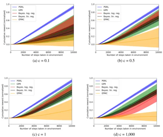
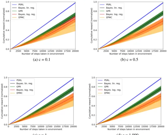
We validate the empirical performance of DUELINGPOSTERIORSAMPLING(DPS) on two simulated domains with varying levels of preference noise, as well as using alternative credit assignment models. We find thatDPSgenerally performs well and outperforms standard PBRL baselines [49].
Experimental setup.We evaluate on two simulated environments: RiverSwim and random MDPs. The RiverSwim environment [29] has six states and two actions (actions 0 and 1); the optimal policy is to always choose action 1, which maximizes the probability of reaching a particular goal state/action pair. Meanwhile, a suboptimal policy—yielding a much smaller reward compared to the goal—is quickly and easily discovered and incentivizes the agent to always select action 0. The algorithm must demonstrate sufficient exploration to have hope of discovering the optimal policy quickly. In the second simulated environment, we generate random MDPs as in [29] with 10 states and 5 actions. The transition dynamics and rewards are generated from Dirichlet (all parameters set to 0.1) and exponential (rate parameter set to 5) distributions, respectively. The parameter for these distributions were chosen to generate MDPs with sparse dynamics and rewards. The sampled reward vectors were shifted and normalized so that the minimum reward is zero and their mean is one. In both of these environments, preferences between pairs of trajectories were generated by (noisily) comparing the total rewards that they accumulated; this reward information was hidden from the learning algorithm, which observed only the trajectory preferences and state transitions. Preference noise is generated according to a logistic model: for trajectoriesτi andτj,P(τi > τj) = {1 +
(a) RiverSwim,c= 1,000 (b) RiverSwim,c= 1 (c) Random MDP,c= 1
Figure 1: Empirical performance ofDPS. a) and b) show RiverSwim with noise hyperparameters
c =1,000, 1. c) displays random MDPs withc = 1. Posterior sampling RL (PSRL) [29] is an upper bound that receives numerical rewards; Gaussian process regression (GPR), Bayesian linear regression, and Bayesian logistic regression are all instances ofDPS. EPMC is a baseline from [50] as discussed. Plots display mean +/- one std over 100 runs of each algorithm tested. Additional results (more values ofc) are in Appendix A3. Normalization is with respect to the total reward achieved by the optimal policy. Overall, we see thatDPSperforms well and is robust to the choice of credit assignment model.
exp[−c(r(τi)−r(τj))]}−1, wherer(τi)andr(τ
j)are the total rewards accrued by the two trajectories, respectively, while the hyperparameterccontrols the degree of noisiness.
Methods compared.We evaluateDPS under four different noise levels (c∈ {0.1,0.5,1,1000}) and three credit assignment models: 1) Bayesian logistic regression, 2) Bayesian linear regression, and 3) Gaussian process regression, where the latter two methods are described in Appendix A1. In addition, we evaluate the Every-Visit Preference Monte Carlo (EPMC) algorithm with probabilistic credit assignment [50, 47] as a baseline. Lastly, we compare against the posterior sampling RL algorithm [29], which learns using the true numerical rewards at each step, and thus yields an upper-bound on the performance that a preference-based algorithm could achieve.
Results. Figure 1 shows the performance comparison forc= 1in both environments, as well as
c= 1,000in RiverSwim (additional results are in Appendix A3, including hyperparameter details). DPSperforms well in all simulations, and significantly outperforms the EPMC baseline. This may be because the EPMC algorithm uses a uniform exploration strategy, whileDPSprioritizes exploration by sampling high rewards in more uncertain regions of the state/action space. Notice thatc=1,000 results in nearly-noiseless preferences; this can decrease performance in RiverSwim in some cases, since preference noise can help the agent to escape the local minimum. We also see thatDPSis competitive with PSRL, which has access to the full cardinal rewards at each state/action. Finally, we see that the performance ofDPSis robust to the choice of credit assignment model, and in fact using Gaussian process regression (for which we do not have an end-to-end regret analysis) often leads to the best empirical performance. These results suggest thatDPSis a practically promising approach that can robustly incorporate many modeling approaches as subroutines.
7
Conclusion
We investigate the preference-based reinforcement learning problem, which receives comparative preferences instead of absolute real-valued rewards as feedback. We develop the DUELING POS-TERIORSAMPLING(DPS) algorithm, which optimizes policies in an highly efficient and flexible way. To our knowledge,DPSis the first preference-based RL algorithm with a regret guarantee. DPSalso performs well in our simulations, and seems practically promising. That makes it both a theoretically-justified and practically promising algorithm.
There are many directions for future work. The Bayesian logistic regression model could be improved with more accurate posterior estimates. Assumptions governing the user’s preferences, such as requiring an underlying utility model, could be relaxed. One can also incorporate kernelized methods to further improve sample efficiency. It is also important to extend to other credit assignment models, such as the Gaussian process regression and Bayesian linear regression methods, for which the same concept of the regret decomposition still applies. We expect thatDPSwould perform well with any asymptotically consistent reward model that sufficiently captures users’ preference behavior.
Acknowledgments
This work was supported by NIH grant EB007615 and an Amazon graduate fellowship.
References
References
[1] Shipra Agrawal and Randy Jia. Optimistic posterior sampling for reinforcement learning: Worst-case regret bounds. InAdvances in Neural Information Processing Systems, pages 1184–1194, 2017.
[2] Nir Ailon, Zohar Karnin, and Thorsten Joachims. Reducing dueling bandits to cardinal bandits. InInternational Conference on Machine Learning, pages 856–864, 2014.
[3] Riad Akrour, Marc Schoenauer, and Michèle Sebag. APRIL: Active preference learning-based reinforcement learning. InJoint European Conference on Machine Learning and Knowledge Discovery in Databases, pages 116–131. Springer, 2012.
[4] Riad Akrour, Marc Schoenauer, Michèle Sebag, and Jean-Christophe Souplet. Programming by feedback. InInternational Conference on Machine Learning, volume 32, pages 1503–1511. JMLR. org, 2014.
[5] James H Albert and Siddhartha Chib. Bayesian analysis of binary and polychotomous response data.Journal of the American statistical Association, 88(422):669–679, 1993.
[6] Dario Amodei, Chris Olah, Jacob Steinhardt, Paul Christiano, John Schulman, and Dan Mané. Concrete problems in AI safety. arXiv preprint arXiv:1606.06565, 2016.
[7] Brenna D Argall, Sonia Chernova, Manuela Veloso, and Brett Browning. A survey of robot learning from demonstration.Robotics and autonomous systems, 57(5):469–483, 2009.
[8] Chandrayee Basu, Qian Yang, David Hungerman, Mukesh Sinahal, and Anca D Dragan. Do you want your autonomous car to drive like you? In2017 12th ACM/IEEE International Conference on Human-Robot Interaction (HRI, pages 417–425. IEEE, 2017.
[9] Christopher Burges, Tal Shaked, Erin Renshaw, Ari Lazier, Matt Deeds, Nicole Hamilton, and Gregory N Hullender. Learning to rank using gradient descent. InProceedings of the 22nd International Conference on Machine learning (ICML-05), pages 89–96, 2005.
[10] Christopher J Burges, Robert Ragno, and Quoc V Le. Learning to rank with nonsmooth cost functions. InAdvances in neural information processing systems, pages 193–200, 2007.
[11] Róbert Busa-Fekete, Balázs Szörényi, Paul Weng, Weiwei Cheng, and Eyke Hüllermeier. Preference-based evolutionary direct policy search. InICRA Workshop on Autonomous Learning, 2013.
[12] Olivier Chapelle and Lihong Li. An empirical evaluation of Thompson sampling. InAdvances in neural information processing systems, 2011.
[13] Paul F Christiano, Jan Leike, Tom Brown, Miljan Martic, Shane Legg, and Dario Amodei. Deep reinforcement learning from human preferences. InAdvances in Neural Information Processing Systems, pages 4299–4307, 2017.
[14] Wei Chu and Zoubin Ghahramani. Preference learning with Gaussian processes. InProceedings of the 22nd international conference on Machine learning, pages 137–144. ACM, 2005.
[15] Miroslav Dudík, Katja Hofmann, Robert E Schapire, Aleksandrs Slivkins, and Masrour Zoghi. Contextual dueling bandits. InConference on Learning Theory (COLT), 2015.
[16] Bianca Dumitrascu, Karen Feng, and Barbara Engelhardt. PG-TS: Improved Thompson sampling for logistic contextual bandits. InAdvances in Neural Information Processing Systems, pages 4624–4633, 2018.
[17] Brochu Eric, Nando D Freitas, and Abhijeet Ghosh. Active preference learning with discrete choice data. InAdvances in neural information processing systems, pages 409–416, 2008.
[18] Johannes Fürnkranz, Eyke Hüllermeier, Weiwei Cheng, and Sang-Hyeun Park. Preference-based reinforcement learning: A formal framework and a policy iteration algorithm. Machine learning, 89(1-2):123–156, 2012.
[19] Subhashis Ghosal et al. Asymptotic normality of posterior distributions in high-dimensional linear models.Bernoulli, 5(2):315–331, 1999.
[20] Aditya Gopalan and Shie Mannor. Thompson sampling for learning parameterized Markov decision processes. InConference on Learning Theory, pages 861–898, 2015.
[21] Christian Gourieroux and Alain Monfort. Asymptotic properties of the maximum likelihood estimator in dichotomous logit models.Journal of Econometrics, 17(1):83–97, 1981.
[22] R Herbrich, T Graepel, and K Obermayer. Support vector learning for ordinal regression. In 1999 Ninth International Conference on Artificial Neural Networks ICANN 99.(Conf. Publ. No. 470), volume 1, pages 97–102. IET, 1999.
[23] Neil Houlsby, Ferenc Huszár, Zoubin Ghahramani, and Máté Lengyel. Bayesian active learning for classification and preference learning.arXiv preprint arXiv:1112.5745, 2011.
[24] Thomas Jaksch, Ronald Ortner, and Peter Auer. Near-optimal regret bounds for reinforcement learning.Journal of Machine Learning Research, 11(Apr):1563–1600, 2010.
[25] Thorsten Joachims. A support vector method for multivariate performance measures. In Proceedings of the 22nd international conference on Machine learning, pages 377–384. ACM, 2005.
[26] Andras Kupcsik, David Hsu, and Wee Sun Lee. Learning dynamic robot-to-human object handover from human feedback. InRobotics research, pages 161–176. Springer, 2018.
[27] Tie-Yan Liu et al. Learning to rank for information retrieval. Foundations and TrendsR in Information Retrieval, 3(3):225–331, 2009.
[28] Kevin P Murphy.Machine learning: A probabilistic perspective. The MIT Press, 2012.
[29] Ian Osband, Daniel Russo, and Benjamin Van Roy. (More) efficient reinforcement learning via posterior sampling. InAdvances in Neural Information Processing Systems, pages 3003–3011, 2013.
[30] Ian Osband and Benjamin Van Roy. Why is posterior sampling better than optimism for reinforcement learning? InProceedings of the 34th International Conference on Machine Learning-Volume 70, pages 2701–2710. JMLR. org, 2017.
[31] Filip Radlinski and Thorsten Joachims. Query chains: Learning to rank from implicit feedback. InProceedings of the eleventh ACM SIGKDD international conference on Knowledge discovery in data mining, pages 239–248. ACM, 2005.
[32] Siddartha Y Ramamohan, Arun Rajkumar, and Shivani Agarwal. Dueling bandits: Beyond con-dorcet winners to general tournament solutions. InAdvances in Neural Information Processing Systems, pages 1253–1261, 2016.
[33] Karthik Raman, Thorsten Joachims, Pannaga Shivaswamy, and Tobias Schnabel. Stable coactive learning via perturbation. InInternational Conference on Machine Learning, pages 837–845, 2013.
[34] Carl Edward Rasmussen and Christopher K Williams. Gaussian processes for machine learning. The MIT Press, 2(3):4, 2006.
[35] Diederik M Roijers, Luisa M Zintgraf, and Ann Nowé. Interactive Thompson sampling for multi-objective multi-armed bandits. InInternational Conference on Algorithmic Decision Theory, pages 18–34. Springer, 2017.
[36] Dorsa Sadigh, Anca D Dragan, Shankar Sastry, and Sanjit A Seshia. Active preference-based learning of reward functions. InRobotics: Science and Systems (RSS), 2017.
[37] Steven L Scott. A modern Bayesian look at the multi-armed bandit.Applied Stochastic Models in Business and Industry, 26(6):639–658, 2010.
[38] Pannaga Shivaswamy and Thorsten Joachims. Online structured prediction via coactive learning. In Proceedings of the 29th International Conference on Machine Learning, pages 59–66. Omnipress, 2012.
[39] Pannaga Shivaswamy and Thorsten Joachims. Coactive learning. Journal of Artificial Intelli-gence Research, 53:1–40, 2015.
[40] Yanan Sui, Vincent Zhuang, Joel Burdick, and Yisong Yue. Stagewise safe Bayesian optimiza-tion with Gaussian processes. InProceedings of the 35th International Conference on Machine Learning, volume 80 ofProceedings of Machine Learning Research, pages 4781–4789. PMLR, 10–15 Jul 2018.
[41] Yanan Sui, Vincent Zhuang, Joel W Burdick, and Yisong Yue. Multi-dueling bandits with dependent arms. InProceedings of the Conference on Uncertainty in Artificial Intelligence, 2017.
[42] Yanan Sui, Masrour Zoghi, Katja Hofmann, and Yisong Yue. Advancements in dueling bandits. InIJCAI, pages 5502–5510, 2018.
[43] Richard S Sutton and Andrew G Barto.Reinforcement learning: An introduction. MIT press, 2018.
[44] Balázs Szörényi, Róbert Busa-Fekete, Adil Paul, and Eyke Hüllermeier. Online rank elicitation for Plackett-Luce: A dueling bandits approach. InAdvances in Neural Information Processing Systems, pages 604–612, 2015.
[45] William R Thompson. On the likelihood that one unknown probability exceeds another in view of the evidence of two samples.Biometrika, 25(3/4):285–294, 1933.
[46] Aaron Wilson, Alan Fern, and Prasad Tadepalli. A Bayesian approach for policy learning from trajectory preference queries. InAdvances in neural information processing systems, pages 1133–1141, 2012.
[47] Christian Wirth.Efficient Preference-based Reinforcement Learning. PhD thesis, Technische Universität, 2017.
[48] Christian Wirth, Riad Akrour, Gerhard Neumann, and Johannes Fürnkranz. A survey of preference-based reinforcement learning methods. The Journal of Machine Learning Research, 18(1):4945–4990, 2017.
[49] Christian Wirth and Johannes Fürnkranz. EPMC: Every visit preference Monte Carlo for reinforcement learning. InAsian Conference on Machine Learning, pages 483–497, 2013. [50] Christian Wirth and Johannes Fürnkranz. A policy iteration algorithm for learning from
preference-based feedback. InInternational Symposium on Intelligent Data Analysis, pages 427–437. Springer, 2013.
[51] Christian Wirth, Johannes Fürnkranz, and Gerhard Neumann. Model-free preference-based reinforcement learning. InThirtieth AAAI Conference on Artificial Intelligence, 2016.
[52] Huasen Wu and Xin Liu. Double Thompson sampling for dueling bandits. InAdvances in Neural Information Processing Systems, pages 649–657, 2016.
[53] Yisong Yue, Josef Broder, Robert Kleinberg, and Thorsten Joachims. The k-armed dueling bandits problem. Journal of Computer and System Sciences, 78(5):1538–1556, 2012.
[54] Yisong Yue, Thomas Finley, Filip Radlinski, and Thorsten Joachims. A support vector method for optimizing average precision. InProceedings of the 30th annual international ACM SIGIR conference on Research and development in information retrieval, pages 271–278. ACM, 2007.
[55] Masrour Zoghi, Zohar S Karnin, Shimon Whiteson, and Maarten De Rijke. Copeland dueling bandits. InAdvances in Neural Information Processing Systems, pages 307–315, 2015.
[56] Masrour Zoghi, Shimon Whiteson, Remi Munos, and Maarten De Rijke. Relative upper confidence bound for the k-armed dueling bandit problem. InInternational Conference on Machine Learning (ICML), 2014.
A1
Bayesian state/action credit assignment: two additional approaches
Credit assignment[48] is the problem of inferring which states or state/action pairs are responsible for observed user preferences. This paper derives theoretical guarantees for a Bayesian logistic regression credit assignment model. In this Appendix, we detail two additional credit assignment models—employing Bayesian linear regression and Gaussian process regression, respectively—for inferring a posterior over state/action utilities using trajectory preferences. (Note that these methods could similarly model utilities over states, rather than state/action pairs.)
In what follows,s˜denotes a state/action pair, withD =SArepresenting the number of possible values ofs˜. For each trajectoryτ ={s˜1,s˜2,˜s3, . . . ,˜sh}, we observe the user’s preference, yielding a dataset{τi|i∈1, . . . , N}ofN labeled trajectories. DefineX ∈RN×Dsuch thatxij := [X]ij is the number of times that trajectoryivisits state/action˜sj. Finally, we denote the label vector as
y∈ {0,1}N, where theithelementy
iis the preference label corresponding toτi; for instance, ifτ1
is preferred toτ2, then we would havey1= 1andy2= 0.
As before,r(˜s)represents the true state/action utilities, such thatr(τ) =Ph
i=1r(˜si), withr(τ)being
trajectoryτ’s total (unobserved) utility. To apply regression methods to this data using preference labels, we approximateyi≈r(τi)to inferr(˜s). In the following, we denoterˆ(˜s)as our model of the true utilitiesr(˜s). Also, definerˆ∈RDas a vector in which theithelement isrˆ(˜si).
In the following, we discuss how to perform Bayesian inference onr(˜s) usingr(τi), which is approximated in practice via preferences. Note that the approximationyi ≈r(τi)performs well empirically, though future work could perhaps apply Bayesian methods such as those in [14] to infer trajectories’ total utilities from the preference labels.
A1.1 Bayesian linear regression
One can estimate state/action utilities from preferences via linear regression:y=Xrˆ+ε, where
εis a vector of residuals and the other quantities are defined above. Bayesian linear regression infers a distribution over likely values ofrˆ. We define conjugate Gaussian prior and likelihood distributions over the state/action utilities and preference labels, respectively, to obtain a Gaussian posterior distribution overrˆ. The prior, likelihood, and posterior take the following form, where Λ ∈ RD×Dandσ∈ Rare prior parameters,Λis positive definite, and we setΛ =λIfor some
λ >0: Prior:rˆ∼ N(0,Λ−1),Λ =λI; Likelihood: p(y|X,rˆ;σ2) = 1 (2πσ2)N2 exp − 1 2σ2||y−Xˆr|| 2 Posterior:rˆ|X,y, σ2,Λ∼ N(µ,Σ), where: (12) µ= (XTX+σ2λI)−1XTy (13) Σ =σ2(XTX+σ2λI)−1 (14)
A1.2 Gaussian process regression
Gaussian process regression [34] extends Bayesian linear regression credit assignment to larger state and action spaces by generalizing across nearby states and actions. We will model the state/action utilitiesrˆ(˜s)as a Gaussian process [34] overs˜, and then use the observed preferences to perform Gaussian process inference onrˆ.
We modelrˆas a Gaussian process:rˆ∼ GP(µr, Kr), whereµris the prior mean vector andKris the prior covariance matrix, such that[Kr]ijgives the prior covariance betweenˆr(˜si)andrˆ(˜sj). We modelr(τi), the total utility for trajectoryτi, as a sum over the latent state/action utilities:
r(τi) = D
X
j=1
with i.i.d. residualsεi∼ N(0, σε2). Because any linear combination of jointly Gaussian variables is Gaussian,r(τi)is a Gaussian process over thexij’s . LetR∈RN be the vector withithelement
equal toRi=r(τi). Calculating the relevant expectations and covariances (see A1.3), one can show thatrˆandRare jointly normally distributed as follows:
ˆ r R ∼ N µr Xµr , Kr KrXT XKT r XKrXT +σε2I . (16)
The standard approach for obtaining a conditional distribution from a joint Gaussian distribution [34] yieldsrˆ|R∼ N(µ,Σ), where: µ=µr+KrXT[XKrXT +σε2I] −1(R−Xµ r) (17) Σ =Kr−KrXT[XKrXT +σ2εI] −1XKT r. (18)
In practice,Ris substituted withyto perform the inference.
A1.3 Using Gaussian processes to infer state/action utilities from preferences
This section derives the posterior inference equations (17) and (18), used in Gaussian process credit assignment. In this derivation, we act as though we observe the trajectories’ total utilitiesR, while remembering that in practice,Ris approximated via the user’s preferences. Recall thatrˆ∈RD
hasith elementrˆ(˜si), which models the utility of state/actioni, whileR ∈
RN has ith element
Ri=r(τi). Letxibe the transpose of theithrow ofX.
Our goal is to infer the values ofˆrgiven observationsRof the trajectories’ total utilities. This can be accomplished via the following four steps:
1. Model the state/action utilitiesrˆ(˜s)as a Gaussian process overs˜.
2. Model the trajectory utilitiesRas a Gaussian process that can be defined as a sum of the state/action utilitiesrˆ(˜s).
3. Using the two Gaussian processes defined in 1) and 2), obtain the covariance matrix between the values of{rˆ(˜s)|s˜∈1, . . . , D}and{Ri|i∈1, . . . , N}.
4. Write the joint Gaussian distribution between the values of {rˆ(˜s)|s˜ ∈ 1, . . . , D} and
{Ri|i∈1, . . . , N}, and obtain the posterior distribution ofrˆat all state/actions givenR. The four subsequent subsections correspond to these four steps, respectively.
A1.3.1 The state/action utility Gaussian process
We model the state/action utilities as a Gaussian process over˜s, with meanE[ˆr(˜s)] =µr(˜s)and covariance kernelCov(ˆr(˜s),rˆ(˜s0)) =kr(˜s,˜s0), for all state/action pairss,˜ s˜0. Thus,
ˆ
r(˜s)∼ GP(µr(˜s), kr(˜s,s˜0)). (19) Defineµr ∈ RD such that the ith element is[µr]i = µr(˜si), the prior mean for the utility of
state/action ˜si. LetKr ∈ RD×D be the covariance matrix over state/action utilities, such that
[Kr]ij=kr(˜si,˜sj). Therefore,rˆ, the vector for which[rˆ]i= ˆr(˜si), is also a Gaussian process:
ˆ
r∼ GP(µr, Kr). (20)
A1.3.2 The trajectory utility Gaussian process
By assumption, the trajectory utilitiesR∈RN are sums of the latent state/action utilities via the following relationship betweenRandrˆ:
R(xi) :=Ri= D
X
j=1
xijˆr(˜sj) +εi, (21)
Note that R(xi)is a Gaussian process overxi ∈ RD because {rˆ(˜s),∀˜s} are jointly normally
distributed by definition of a Gaussian process, and any linear combination of jointly Gaussian variables has a univariate normal distribution.
Next, we calculate the expectation and covariance ofRover the observations. The expectation of its
ithelementR
i=R(xi)can be expressed as follows:
E[Ri] =E D X j=1 xijrˆ(˜sj) +εi = D X j=1 xijE[ˆr(˜sj)] = D X j=1 xijµr(˜sj). (22)
The expectation overR(X)can thus be written as:
E[R(X)] =Xµr. (23)
Next, we model the covariance matrix ofR(X). Theijthelement of this matrix is the covariance of
R(xi)andR(xj): Cov(R(xi), R(xj)) =E[R(xi)R(xj)]−E[R(xi)]E[R(xj)] (24) =E[R(xi)R(xj)]− D X k=1 xikµr(˜sk) ! D X m=1 xjmµr(˜sm) ! (25) =E " D X k=1 xikˆr(˜sk) +εi ! D X m=1 xjmrˆ(˜sm) +εj !# (26) − D X k=1 xikµr(˜sk) ! D X m=1 xjmµr(˜sm) ! (27) = D X k=1 D X m=1 xikxjmE[ˆr(˜sk)ˆr(˜sm)] +E[εiεj]− D X k=1 D X m=1 xikxjmµr(˜sk)µr(˜sm) (28) = D X k=1 D X m=1 xikxjm[Cov(ˆr(˜sk),rˆ(˜sm)) +µr(˜sk)µr(˜sm)] (29) − D X k=1 D X m=1 xikxjmµr(˜sk)µr(˜sm) +σε2I[i=j] (30) = D X k=1 D X m=1 xikxjmCov(ˆr(˜sk),rˆ(˜sm)) +σε2I[i=j] (31) = D X k=1 D X m=1 xikxjmkr(˜sk,s˜m) +σ2εI[i=j] =xTi Krxj+σ2εI[i=j]. (32)
We can then write the covariance matrix ofRasKR(X), where:
[KR(X)]ij= Cov(R(xi), R(xj)) =xTi Krxj+σε2I[i=j]. (33)
From here, it can be seen thatKR(X) =XKrXT +σε2I:
XKrXT = xT1 xT 2 .. . xT N Kr[x1 x2 . . . xN] = xT1 xT 2 .. . xT N [Krx1 Krx2 . . . KrxN] (34) = xT 1Krx1 . . . xT1KrxN .. . . .. ... xT NKrx1 . . . xTNKrxN =KR(X)−σ 2 εI. (35)
A1.3.3 Covariance between state/action and trajectory utilities
In this subsection, we consider the covariance betweenrˆandR, denotedKˆr,R:
[Kˆr,R]ij = Cov([rˆ]i,[R]j) = Cov(ˆr(˜si), R(xj)). (36)
This covariance matrix can be expressed in terms ofX, Kr, andµr:
[Kˆr,R]ij = Cov(ˆr(˜si), R(xj)) = Cov rˆ(˜si), D X k=1 xjkrˆ(˜sk) +εj ! (37) =E " ˆ r(˜si) D X k=1 xjkˆr(˜sk) +εjrˆ(˜si) # −E[ˆr(˜si)]E " D X k=1 xjkrˆ(˜sk) +εj # (38) = D X k=1 xjkE[ˆr(˜si)ˆr(˜sk)]−[µr(˜si)][xTjµr] (39) = D X k=1 xjk{Cov(ˆr(˜si),ˆr(˜sk)) +E[ˆr(˜si)]E[ˆr(˜sk)]} −µr(˜si)xTjµr (40) = D X k=1 xjk[kr(˜si,s˜k) +µr(˜si)µr(˜sk)]−µr(˜si)xTjµr (41) = D X k=1 xjkkr(˜si,s˜k) +µr(˜si)xTjµr−µr(˜si)xTjµr = D X k=1 xjkkr(˜si,s˜k) =xTj[Kr]i,:, (42)
where[Kr]i,:is the column vector obtained by transposing theithrow ofKr. From here, one can see
thatKˆr,R=KrXT: KrXT = [Kr]T1,: [Kr]T 2,: .. . [Kr]TD,: ∗[x1 x2 . . . xN] =Kˆr,R. (43)
A1.3.4 Posterior inference over state/action utilities
The results of the previous three subsections can be combined to obtain the following joint probability density betweenrˆandR:
ˆ r R ∼ N µr Xµr , Kr KrXT XKrT XKrXT +σε2I . (44)
This relationship expresses all components of the joint Gaussian density in terms ofX, Kr, andµr,
or in other words, in terms of the state/action visit counts in the observed trajectories (captured byX) and the Gaussian process prior onrˆ.
Using the standard approach for obtaining a conditional distribution from a jointly Gaussian distribu-tion (see Appendix A.2 in [34]), we arrive at:
ˆ r|R∼ N(µ,Σ), where: (45) µ=µr+KrXT[XKrXT +σε2I] −1(R−Xµ r) (46) Σ =Kr−KrXT[XKrXT +σε2I] −1XKT r. (47)
Thus, we have expressed the conditional posterior density ofrˆin terms ofX, Kr, µr, and the
A2
Proofs
This section proves the theoretical results stated in Section 5 of the paper.
We begin by restating a result from Gourieroux and Monfort [21] establishing conditions in which logistic regression is asymptotically consistent, after defining two necessary conditions.
Definition 1(Derivative of sigmoid). f :R−→R, wheref = (1+ee−−xx)2. Note thatf(x) =f(−x). This is the derivative of the sigmoid function,σ(x) = 1+1e−x.
Definition 2. Letr∈RDbe the vector of true state/action utilities (assumed to exist) andr0∈RD−1
be its transformation via(4). Define ˜r0k ∈ RD−1 as the state/action rewards sampled from the
Bayesian logistic regression model posterior in episodek,rˆk0 ∈RD−1as the model’s maximum a posteriori (MAP) estimate at episodek, andrˆ0M L,k∈RD−1as its maximum likelihood estimate atk.
Lastly,r˜k∈RD,rˆk ∈RD, andrˆM L,k∈RDare their respective equivalents given by(5).
Condition 1. ∃m0<∞such that|zij| ≤m0for alli∈ {1, . . . , N}, j∈ {1, . . . , D−1}.
Condition 1 is always satisfied becausezij=xTivjby (4), wherevjis a unit vector. Additionally,
xi=x1i−xi2is difference of two vectors that both count how many times each state/action pair is
visited in an episode, and thus both have only positive elements that sum to the episode horizon,h. So,|zij| ≤ ||xi||2||vj||2=||xi||2≤ ||x1i−xi2||1=||x1i||+||xi2||1= 2h, where the inequalities
are respectively the Cauchy-Schwarz inequality, ||x||p < ||x||q forp > q > 0, and the triangle inequality. So, Condition 1 holds form0= 2h.
Condition 2. Let λ(1k) and λ(D−k)1 be the largest and smallest eigenvalues, respectively, of
Pk
i=1f(ziTr
0)z
iziT. Then,∃m1<∞such that
λ(k)1
λ(k)D−1 < m1, for all k.
Intuitively, Condition 2 requires that an arbitrarily-high fraction of observationscannot lie in a proper subspace of their possible span. This condition is necessary, as otherwise data outside this subspace would become increasingly ignored as more data points are obtained. Condition 2 states that the inverse Hessian of the negative log reward posterior—evaluated at the true rewardsr0—has an upper-bounded ratio between its largest and smallest eigenvalues. This can be explicitly enforced by bounding this maximum-to-minimum eigenvalue ratio for the matrixPk
i=1f(z
T
i rˆ0k)ziziT, and only updating the reward posterior when the eigenvalue ratio is below-threshold. As shown in Lemma 1 below, satisfying this restriction bounds the eigenvalue ratio forPk
i=1f(z
T i r
0)z
iziT, as desired. Condition 2 may also be guaranteed in certain situations, e.g., if randomness in the dynamics is sufficient to ensure a full-row-rank observation matrix Z. In this case, the eigenvalue ratio will be bounded regardless of the specific policies executed. If properties of the environment are known to guarantee Condition 2, then it need not be explicitly enforced. Meanwhile, weakening the requirements of Condition 2—for instance, by strengthening the Bayesian logistic regression convergence analysis or considering other credit assignment models—would be an interesting avenue for future work.
Lemma 1(Enforcing Condition 2). The eigenvalue ratio λmax(
Pk i=1f(z T ir 0)z izTi) λmin(Pki=1f(ziTr0)ziziT) has a constant upper bound that holds for allkif and only if the eigenvalue ratio λmax(
Pk i=1f(z T irˆ 0 k)zizTi) λmin(Pki=1f(zTirˆ0k)zizTi) has a constant upper bound that holds for allk. Therefore, one can ensure that the former condition holds by enforcing the latter.
Proof. We apply the result in Lemma 1.1 below. To verify that the conditions for this result hold, we must show that bothf(zT
i r0)andf(ziTrˆ0k)have upper and lower bounds for alli, k, where the lower bound exceeds zero. The upper bound exists becausef(x)∈(0,1]∀x.
It remains to show that bothf(zT
i r0)andf(zTi rˆ0k)are lower-bounded above zero. Becausef(x) monotonically decreases as|x|increases, this is true as long as|ziTr0|and|ziTrˆk0|are upper-bounded. In the former case,|zT
i r
0| <||z
i||2||r0||2. The quantity||zi||2is upper-bounded by Condition 1.
The rewardsr0produce the same policy when scaled by any positive quantity, and so their magnitude can be viewed as fixed. The same logic holds in the latter case.
Lemma 1.1(Bounded eigenvalue ratios). LetAk, Bk ∈Rn×nbe two matrices of the formAk =
Pk
i=1αivivTi ,Bk=P k
i=1βiviviT, whereαi∈[αmin, αmax], βi ∈[βmin, βmax],αmin>0, βmin>0, andvi∈Rnfori∈ {1, . . . , k}. Letλmax(M)andλmin(M)respectively be the largest eigenvalues
of a matrixM. Then, λmax(Ak)
λmin(Ak) is upper-bounded for allTif and only if
λmax(Bk)
λmin(Bk) is upper-bounded for allT.
Proof. Without loss of generality, we assume that λmax(Ak)
λmin(Ak) < m1 <∞for somem1and for all
k, and will show that λmax(Bk)
λmin(Bk) has an upper bound for allk. Note thatauu
T 0(i.e., is positive semidefinite) for anya >0and vectoru, and that sums of positive semidefinite matrices are also positive semidefinite. In addition, we will use the following facts about arbitrary positive semidefinite matricesA, B0(which can be shown from the Courant-Fischer-Weyl min-max principle):
λmax(A)≤λmax(A+B) (48)
λmin(A)≤λmin(A) +λmin(B)≤λmin(A+B) (49)
The desired result is an outcome of the following four relations:
λmax(Ak) =λmax k X i=1 αivivTi ! =λmax k X i=1 (αi−αmin)vivTi + k X i=1 αminvivTi ! (50) ≥λmax k X i=1 αminvivTi ! =αminλmax k X i=1 viviT ! , by (48) (51) λmin(Ak) =λmin k X i=1 αiviviT ! ≤λmin k X i=1 αiviviT ! +λmin k X i=1 (αmax−αi)vivTi ! (52) ≤λmin k X i=1 αmaxvivTi ! =αmaxλmin k X i=1 viviT ! , by (49) (53) λmax(Bk) =λmax k X i=1 βivivTi ! ≤λmax k X i=1 βivivTi + k X i=1 (βmax−βi)vivTi ! , by (48) (54) =λmax k X i=1 βmaxvivTi ! =βmaxλmax k X i=1 viviT ! (55) λmin(Bk) =λmin k X i=1 βiviviT ! =λmin k X i=1 (βi−βmin)viviT+ k X i=1 βminvivTi ! (56) ≥λmin k X i=1 βminviviT ! =βminλmin k X i=1 viviT ! , by (49) (57)
Now, we can upper bound the eigenvalue ratio forBk:
λmax(Bk) λmin(Bk) ≤ βmaxλmaxPk i=1viviT βminλminPk i=1viviT , by (55) and (57) (58) ≤ βmax βmin λmax(Ak) αmin λ min(Ak) αmax −1 , by (51) and (53) (59) = βmaxαmax βminαmin λmax(Ak) λmin(Ak) ≤ βmaxαmax βminαmin ∗m1. (60)
We will apply the following result from Gourieroux and Monfort [21] concerning asymptotic consis-tency of the maximum likelihood estimator:
Proposition 1(Asymptotic consistency of logistic regression [21]). If Conditions 1 and 2 are satisfied, then the maximum likelihood estimatorˆrM L,k0 ofr0exists almost surely ask−→ ∞, andrˆM L,k0
converges almost surely to the true valuer0if and only if lim k−→∞λ
(k)
D−1=∞.
Proof. This result is a restatement of Proposition 3 in Gourieroux and Monfort [21].
Remark: The proof of Proposition 1 in [21] can be adapted such that the same result holds when the maximum likelihood estimatorrˆM L,k0 is replaced with the MAP estimatorrˆ0k; thus, it applies to our setting. We show that Proposition 1’s final condition for convergence of the MAP estimator holds: Lemma 2. Under known transition dynamics, all eigenvalues of the matrixPk
i=1f(z
T
i r0)ziziT approach infinity ask−→ ∞.
Proof. Letαi = f(ziTr0) andαˆ
(k)
i = f(yiziTrˆ0k). The values αi are both upper-bounded and non-decaying:f(x)∈(0,1)for allx, andzT
i r0is bounded in magnitude since we assume the true rewardsr0are bounded. We can write:
N X i=1 f(ziTr0)zizTi = N X i=1 αiziziT = [ √ α1z1 √ α2z2 . . . √ αNzN] √ α1z1T √ α2z2T .. . √ αNzNT . (61)
DefineM ∈RN×(D−1),M1∈Rm×(D−1), andM2∈R(N−m)×(D−1)as:
M = √ α1z1T √ α2z2T .. . √ αNzTN , M1= √ α1z1T √ α2z2T .. . √ αmzTm , M2= √ αm+1zmT+1 .. . √ αNzNT . (62) Then, M = M1 M2 , andMTM = N X i=1 αizizTi =M1TM1+M2TM2. (63) Also, define Mˆ ∈ RN×(D−1), Mˆ
1 ∈ Rm×(D−1), andMˆ2 ∈ R(N−m)×(D−1)analogously, but
replacingαiwithαˆ
(N)
i . Note thatM
TMandMˆTMˆ have the same rank, sinceM andMˆ have the same row-rank; similarlyMTM
iandMˆiTMˆihave the same rank fori∈ {1,2}. Assume that there existsm∈Nsuch thatMˆT
2Mˆ2has rank less than(D−1); letr≥1be the number
of zero eigenvalues ofMˆT
2Mˆ2. We will show that asNincreases, the probability of drawing a sample
zithat is linearly independent of the rows already inMˆ2(that is, a sample that increases the rank
ofMT
2M2) does not decay to zero. This means that there will be infinitely-many non-overlapping
sets of indices{j, . . . , k}such thatPk
i=jαizizTi has rank(D−1). From here, we can show that (D−1)of the eigenvalues ofMTM approach infinity (recall that theαivalues are lower-bounded). Under the Laplace approximation, the posterior covariance afterN episodes takes the formΣN =
PN i=1f(yizTi rˆN)ziziT +V −1 0 −1 =MˆTMˆ +V−1 0 −1
. Under our assumption thatMˆT
2Mˆ2
hasr≥1eigenvalues equal to zero, the row-rank ofMˆ2is(D−1−r).
We show thatΣN hasreigenvalues that are bounded away from zero. We write the eigenvalues of any square matrixM0 ∈ Rn×n asλ1(M0) ≥λ2(M0) ≥. . . ≥λn(M0). Then, we apply the
following fact (which can be shown from the Courant-Fischer-Weyl min-max principle): for positive semidefinite matricesA, B∈Rn×n, λn(A) +λk(B)≤λk(A+B)≤λ1(A) +λk(B). (64) Clearly, PN i=1αˆ (N) i ziziT and V −1
0 are both positive semidefinite (V0 is positive definite by its
definition), and so:
0≤λk N X i=1 ˆ α(iN)ziziT +V −1 0 ! ≤λ1 V0−1 +λk N X i=1 ˆ α(iN)zizTi ! , (65)
where the first inequality holds because the sum of two positive semidefinite matrices is also positive semidefinite, and the second inequality is an application of the inequality in (64). The first term in (65) is a constant, while the second is zero fork > D−1−r. Thus,Σ−N1=PN
i=1αˆ (N)
i zizTi +V −1 0
hasreigenvalues that are upper-bounded, where the upper bound depends only onV0. Therefore,Σ
hasreigenvalues that are lower-bounded byλ1 V0−1
−1
=hλ 1 D−1(V0)
i−1
=λD−1(V0)>0; the
otherD−1−reigenvalues ofΣall decay to zero.
To complete the proof, we argue that the following statements hold; the first two of these statements are proven in the two subsequent sub-lemmas; the third statement completes the proof.
1. Note thatMTMandMˆTMˆ have the same rank, due toMandMˆ having the same row-rank. Assume that for somem,Mˆ2TMˆ2hasr≥1zero eigenvalues. The reward vectorr˜0sampled
from the logistic regression posterior can be expressed in terms of the eigenbasis ofMˆT
2Mˆ2, {νi|i = 1, . . . , D−1}: r˜0 =PD−
1
i=1 βiνifor some coefficientsβi. Then, asN −→ ∞, forjsuch thatvjis in the null-space ofMˆ2TMˆ2, the probability of samplingr˜0N such that
|βj|
PD−1 i=1 |βi|
≥bfor anyb∈(0,1)does not decay to zero. 2. There existsb ∈ (0,1)such that if βj
PD−1 i=1 βi
≥ b, then with probability above zero, the policy will sample a trajectory such that the nextzisample has a nonzero component inνj.
3. If a trajectory as described in 2) is sampled, a zero-eigenvalue ofM2TM2increases by a
lower-bounded amount. This comes from the fact that there are only finitely-many possible
zivectors, so ifzihas nonzero inner product with an eigenvector, this inner product cannot be arbitrarily close to zero. This contradicts that Rank(MT
2M2)remains belowD−1as N −→ ∞.
Lemma 2.1(Proof of Statement 1 in Lemma 2).
Proof. In episodeN, the sampled reward vectorr˜N0 is drawn from the logistic regression posterior,
N(rˆ0,ΣN), with covariance matrixΣN =
PN i=1αˆ (N) i ziziT+V −1 0 −1 . Consider a sampler˜0N
with a multivariate normal distribution inRD−1:
N(r˜0N|rˆN0 ,ΣN)∝exp −1 2(r˜ 0 N−rˆN0 ) TΣ−1 N (r˜ 0 N −rˆ0N) . (66)
The intuition for this proof is as follows. There is a decreasing probability of sampling a vectorr˜0N
such that(˜r0
N −rˆ0N)has components in eigenvectors ofΣN whose eigenvalues decay toward zero. Rather, the probability density concentrates toward the span of eigenvectors ofΣN whose eigenvalues are bounded away from zero.
The probability density ofr˜N0 can be viewed as a function of(r˜N0 −rˆN0 )TΣ−1
N (˜r 0 N −rˆ
0
N). This fact can be used to defineRα,N ⊂RD−1:
Forε∈(0,1), defineα0(ε)as the maximum possible value ofαsuch thatP(r˜0∈Rα)≥1−ε: α0(ε) = max
s.t.P(˜r0∈R
α)≥1−ε
α. (68)
Thus,Rα0(ε)contains at least1−εof the probability density of˜r 0 N.
Recall thatΣ−N1hasreigenvalues that are upper-bounded, while the otherD−1−reigenvalues ofΣ−N1all approach infinity asN −→ ∞. Let(λi,µi)represent the eigenvalues and eigenvectors ofΣ−N1, respectively. Then,r˜N0 −rˆN0 can be expressed in terms of the eigenbasis: r˜N0 −rˆN0 =
PD−1
i=1 ηiµifor some coefficientsηi, and:
(r˜N0 −rˆ0N)TΣ−1(r˜0N−rˆN0 ) = D−1
X
i=1
η2iλi. (69)
Then,Rα0(ε)can be written as,
Rα0(ε)= ( ˜ rN0 ∈RL−1 D−1 X i=1 η2iλi≤α0(ε) ) . (70)
We can divider˜0N−rˆN0 forr˜N0 ∈Rα0(ε)into two terms:
˜ rN0 −rˆ0N = D−1−r X i=1 ηiµi+ D−1 X i=D−r ηiµi, (71)
where λi −→ ∞fori ≤ D−1−r. The first term contains eigenvectorsµi corresponding to eigenvalues ofΣ−N1that grow to infinity, while the second term contains eigenvectors corresponding to upper-bounded eigenvalues ofΣ−N1. Forr˜N0 belonging toRα0(ε), asλi−→ ∞, theηicoefficients in the first term will decay; otherwise, the sumPD−1
i=1 η 2
iλigrows unboundedly, whileP D−1
i=1 η 2
iλi remains comparatively-smaller for increasingly-many vectors that place weight only onµi for
i > D−1−r. In other words, asN −→ ∞, the probability density ofr˜N0 −rˆ0N increasingly concentrates toward vectors that can be expressed as linear combinations of eigenvectors ofΣ−N1 corresponding to upper-boundedλi. Thus, as long asλj, j > D−1−r, are upper-bounded, the probability of sampling˜r0N−rˆN0 such that ηj
PD−1
i=1 ηi ≥bfor anyj > D−1−rand anyb∈(0,1) does not decay to zero.
Next, we argue that the eigenvectors ofΣ−N1approach a set of vectors spanning the null space of ˆ
M2TMˆ2asN −→ ∞. Forj≤D−1−r,(λj,µj)is an eigenpair ofΣ−N1for whichλj−→ ∞as
N −→ ∞. The eigenpair relationship gives: N X i=1 ˆ α(iN)ziziT+V −1 0 ! µj =λjµj. (72) Dividing byλj, 1 λj N X i=1 ˆ α(iN)zizTi + 1 λj V0−1 ! µj=µj. (73) The termλ1 jV −1
0 becomes insignificant asλj −→ ∞, sinceV0is constant, while scaling the first
term by λ1
j does not affect its eigenbasis. Thus, forj≤D−1−r,µjapproaches an eigenvector ofPN
i=1αˆ (N)
i zizTi that has an unbounded eigenvector. Meanwhile, the span of eigenvectorsµj forj > D−1−rapproaches the span of eigenvectors ofPN
i=1αˆ (N)
i ziziT with upper-bounded eigenvalues. Equivalently, the span of eigenvectorsµjforj > D−1−rapproaches the null space ofMˆ2TMˆ2=P
N i=m+1αˆ
(N)