Physics Department, University of Wuppertal, D-42097 Wuppertal, Germany Received 30 August 1999; received in revised form 4 January 2000; accepted 4 January 2000
Communicated by E. Ott
Abstract
Before we apply nonlinear techniques, e.g. those inspired by chaos theory, to dynamical phenomena occurring in nature, it is necessary to first ask if the use of such advanced techniques is justified by the data. While many processes in nature seem very unlikely a priori to be linear, the possible nonlinear nature might not be evident in specific aspects of their dynamics. The method of surrogate data has become a very popular tool to address such a question. However, while it was meant to provide a statistically rigorous, foolproof framework, some limitations and caveats have shown up in its practical use. In this paper, recent efforts to understand the caveats, avoid the pitfalls, and to overcome some of the limitations, are reviewed and augmented by new material. In particular, we will discuss specific as well as more general approaches to constrained randomisation, providing a full range of examples. New algorithms will be introduced for unevenly sampled and multivariate data and for surrogate spike trains. The main limitation, which lies in the interpretability of the test results, will be illustrated through instructive case studies. We will also discuss some implementational aspects of the realisation of these methods in the TISEAN software package. © 2000 Elsevier Science B.V. All rights reserved.
PACS: 05.45.+b
Keywords: Time series; Surrogate data; Nonlinearity
1. Introduction
A nonlinear approach to analysing time series data [1–5] can be motivated by two distinct reasons. One is intrinsic to the signal itself while the other is due to additional knowledge we may have about the nature of the observed phenomenon. As for the first motivation, it might be that the arsenal of linear methods has been exploited thoroughly but all the efforts left certain structures in the time series unaccounted for. As for the second, a system may be known to include nonlinear components and therefore a linear description seems unsatisfactory in the first place. Such an argument is often heard for example in brain research — nobody expects for example the brain to be a linear device. In fact, there is ample evidence for nonlinearity, in particular, in small assemblies of neurons. Nevertheless, the latter reasoning is rather dangerous. The fact that a system contains nonlinear components does not prove that this
∗Corresponding author.
0167-2789/00/$ – see front matter © 2000 Elsevier Science B.V. All rights reserved. PII: S 0 1 6 7 - 2 7 8 9 ( 0 0 ) 0 0 0 4 3 - 9
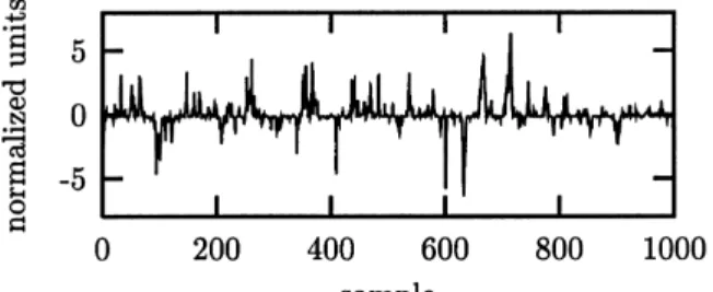
Fig. 1. A time series showing characteristic bursts.
nonlinearity is also reflected in a specific signal we measure from that system. In particular, we do not know if it is of any practical use to go beyond the linear approximation when analysing the signal. After all, we do not want our data analysis to reflect our prejudice about the underlying system but to represent a fair account of the structures that are present in the data. Consequently, for a data driven analysis, the application of nonlinear time series methods has to be justified by establishing nonlinearity in the time series.
Suppose we had measured the signal shown in Fig. 1 in some biological setting. Visual inspection immediately reveals nontrivial structure in the serial correlations. The data fail a test for Gaussianity, thus ruling out a Gaussian linear stochastic process as their source. Depending on the assumptions we are willing to make on the underlying process, we might suggest different origins for the observed strong “spikyness” of the dynamics. Superficially, low dimensional chaos seems unlikely due to the strong fluctuations, but maybe high dimensional dynamics? A large collection of neurons could intermittently synchronise to give rise to the burst episodes. In fact, certain artificial neural network models show qualitatively similar dynamics. The least interesting explanation, however, would be that all the spikyness comes from a distortion by the measurement procedure and all the serial correlations are due to linear stochastic dynamics. Occam’s razor tells us that we should rule out such a simple explanation before we venture to construct more complicated models.
Surrogate data testing attempts to find the least interesting explanation that cannot be ruled out based on the data. In the above example, the data shown in Fig. 1, this would be the hypothesis that the data has been generated by a stationary Gaussian linear stochastic process (equivalently, an autoregressive moving average or ARMA process) that is observed through an invertible, static, but possible nonlinear observation function:
sn=s(xn), {xn}: ARMA(M, N) (1)
Neither the orderM, N, the ARMA coefficients, nor the functions(·)are assumed to be known. Without explicitly modeling these parameters, we still know that such a process would show characteristic linear correlations (reflecting the ARMA structure) and a characteristic single time probability distribution (reflecting the action ofs(·)on the original Gaussian distribution). Fig. 2 shows a surrogate time series that is designed to have exactly these properties in common with the data but to be as random as possible otherwise. By a proper statistical test we can now look for additional structure that is present in the data but not in the surrogates.
In the case of the time series in Fig. 1, there is no additional structure since it has been generated by the rule
sn=αxn3, xn=0.9xn−1+ηn, (2)
where{ηn}are Gaussian independent increments andαis chosen so that the data have unit variance.1 This means
1In order to simplify the notation in mathematical derivations, we will assume throughout this paper that the mean of each time series has
been subtracted and it has been rescaled to unit variance. Nevertheless, we will often transform back to the original experimental units when displaying results graphically.
Fig. 2. A surrogate time series that has the same single time probability distribution and the same autocorrelation function as the sequence in Fig. 1. The bursts are fully explained by these two properties.
that the strong nonlinearity that generates the bursts is due to the distorted measurement that enhances ordinary fluctuations, generated by linear stochastic dynamics.
In order to systematically exclude simple explanations for time series observations, this paper will discuss formal statistical tests for nonlinearity. We will formulate suitable null hypotheses for the underlying process or for the observed structures themselves. In the former case, null hypotheses will be extensions of the statement that the data were generated by Gaussian linear stochastic processes. The latter situation may occur when it is difficult to properly define a class of possibly underlying processes but we want to check if a particular set of observables gives a complete account of the statistics of the data. We will attempt to reject a null hypothesis by comparing the value of a nonlinear parameter taken on by the data with its probability distribution. Since only exceptional cases allow for the exact or asymptotic derivation of this distribution unless strong additional assumptions are made, we have to estimate it by a Monte Carlo resampling technique. This procedure is known in the nonlinear time series literature as the method of surrogate data, see Refs. [6–8]. Most of the body of this paper will be concerned with the problem of generating an appropriate Monte Carlo sample for a given null hypothesis.
We will also dwell on the proper interpretation of the outcome of such a test. Formally speaking, this is totally straightforward: A rejection at a given significance level means that if the null hypothesis is true, there is a certain small probability to still see the structure we detected. Non-rejection means even less: either the null hypothesis is true, or the discriminating statistics we are using fails to have power against the alternative realised in the data. However, one is often tempted to go beyond this simple reasoning and speculate either on the nature of the nonlinearity or non-stationarity that lead to the rejection, or on the reason for the failure to reject.
Since the actual quantification of nonlinearity turns out to be the easiest — or in any case the least dangerous — part of the problem, we will discuss it first. In principle, any nonlinear parameter can be employed for this purpose. They may however differ dramatically in their ability to detect different kinds of structures. Unfortunately, selecting the most suitable parameter has to be done without making use of the data since that would render the test incorrect: If the measure of nonlinearity has been optimised formally or informally with respect to the given data set, a fair comparison with surrogates is no longer possible. Only information that is shared by data and surrogates, i.e., e.g. linear correlations, may be considered for guidance. If multiple data sets are available, one could use some sequences for the selection of the nonlinearity parameter and others for the actual test. Otherwise, it is advantageous to use one of the parameter free methods that can be set up without detailed knowledge of the data.
Since we want to advocate routine use of a nonlinearity test whenever nonlinear methods are planned to be applied, we feel that it is important to make a practical implementation of such a test easily accessible. Therefore, one branch of the TISEAN free software package [9] is devoted to surrogate data testing. Appendix A will discuss the implementational aspects necessary to understand what the programs in the package do.
2. Detecting weak nonlinearity
Many quantities have been discussed in the literature that can be used to characterise nonlinear time series. For the purpose of nonlinearity testing we need such quantities that are particularly powerful in discriminating linear dynamics and weakly nonlinear signatures — strong nonlinearity is usually more easily detectable. An important objective criterion that can be used to guide the preferred choice is the discrimination power of the resulting test. It is defined as the probability that the null hypothesis is rejected when it is indeed false. It will obviously depend on how and how strongly the data actually deviates from the null hypothesis.
2.1. Higher order statistics
Traditional measures of nonlinearity are derived from generalisations of the two-point auto-covariance function or the power spectrum. The use of higher order cumulants as well as bi-and multi-spectra is discussed, e.g. in Ref. [10]. One particularly useful third order quantity2 is
φrev(τ)= 1 N −τ N X n=τ+1 (sn−sn−τ)3, (3)
since it measures the asymmetry of a series under time reversal. (Remember that the statistics of linear stochastic processes is always symmetric under time reversal. This can be most easily seen when the statistical properties are given by the power spectrum which contains no information about the direction of time.) Time reversibility as a criterion for discriminating time series is discussed in detail in Ref. [11], where, however, a different statistic is used to quantify it. The concept itself has quite a folklore and has been used, e.g. in Refs. [6,12].
Time irreversibility can be a strong signature of nonlinearity. Let us point out, however, that it does not imply a dynamical origin of the nonlinearity. We will later (Section 7.1) give an example of time asymmetry generated by a measurement function involving a nonlinear time average.
2.2. Phase space observables
When a nonlinearity test is performed with the question in mind if nonlinear deterministic modeling of the signal may be useful, it seems most appropriate to use a test statistic that is related to a nonlinear deterministic approach. We have to keep in mind, however, that a positive test result only indicates nonlinearity, not necessarily determinism. Since nonlinearity tests are usually performed on data sets which do not show unambiguous signatures of low-dimensional determinism (like clear scaling over several orders of magnitude), it is not very fruitful to use an estimator of one of these quantitative indicators of chaos, like the fractal dimension or the Lyapunov exponent. These algorithms have been optimised to minimise the bias, often at the price of a higher variance. Still, some useful test statistics are at least inspired by these quantities. Usually, some effective value at a finite length scale has to be computed without establishing scaling regions or attempting to approximate the proper limits.
In order to define an observable inm-dimensional phase space, we first have to reconstruct that space from a scalar time series, e.g. by the method of delays:
sn=(sn−(m−1)τ, sn−(m−2)τ, . . . , sn). (4)
2We have omitted the commonly used normalisation to second moments since throughout this paper, time series and their surrogates will have
the major limiting factor for the performance of a statistical indicator is its variance since possible differences between two samples may be hidden among the statistical fluctuations. In Ref. [13], a number of popular measures of nonlinearity are compared quantitatively. The results can be summarised by stating that in the presence of time-reversal asymmetry, the particular quantity, Eq. (3), that derives from the three-point autocorrelation function gives very reliable results. However, many nonlinear evolution equations produce little or no time-reversal asymmetry in the statistical properties of the signal. In these cases, simple measures like a prediction error of a locally constant phase space predictor, Eq. (5), performed best. It was found to be advantageous to choose embedding and other parameters in order to obtain a quantity that has a small spread of values for different realisations of the same process, even if at these parameters no valid embedding could be expected.
Of course, prediction errors are not the only class of nonlinearity measures that have been optimised for robustness. Notable other examples are coarse-grained redundancies [14–16], and, at an even higher level of coarse-graining, symbolic methods [17]. The very popular method of false nearest neighbours [18] can be easily modified to yield a scalar quantity suitable for nonlinearity testing. The same is true for the concept of unstable periodic orbits (UPOs) [19,20].
3. Surrogate data testing
All of the measures of nonlinearity mentioned above share a common property. Their probability distribution on finite data sets is not known analytically — except maybe when strong additional assumptions about the data are made. Some authors have tried to give error bars for measures like predictabilities (e.g. Barahona and Poon [21]) or averages of pointwise dimensions (e.g. Skinner et al. [22]) based on the observation that these quantities are averages (mean values or medians) of many individual terms, in which case the variance (or quartile points) of the individual values yield an error estimate. This reasoning is however only valid if the individual terms are independent, that is usually not the case for time series data. In fact, it is found empirically that nonlinearity measures often do not even follow a Gaussian distribution. Also the standard error given by Roulston [23] for the mutual information is fully correct only for uniformly distributed data. His derivation assumes a smooth rescaling to uniformity. In practice, however, we have to rescale either to exact uniformity or by rank-ordering uniform variates. Both transformations are in general non-smooth and introduce a bias in the joint probabilities. In view of the serious difficulties encountered when deriving confidence limits or probability distributions of nonlinear statistics with analytical methods, it is highly preferable to use a Monte Carlo resampling technique for this purpose.
3.1. Typical vs. constrained realisations
Traditional bootstrap methods use explicit model equations that have to be extracted from the data and are then run to produce Monte Carlo samples. This typical realisations approach can be very powerful for the computation of confidence intervals, provided the model equations can be extracted successfully. The latter requirement is very
delicate. Ambiguities in selecting the proper model class and order, as well as the parameter estimation problem have to be addressed. Whenever the null hypothesis involves an unknown function (rather than just a few parameters) these problems become profound. A recent example of a typical realisations approach to creating surrogates in the dynamical systems context is given by Ref. [24]. There, a Markov model is fitted to a coarse-grained dynamics obtained by binning the two-dimensional delay vector distribution of a time series. Then, essentially the transfer matrix is iterated to yield surrogate sequences. We will offer some discussion of that work later in Section 7.
As discussed by Theiler and Prichard [25], the alternative approach of constrained realisations is more suitable for the purpose of hypothesis testing we are interested in here. It avoids the fitting of model equations by directly imposing the desired structures onto the randomised time series. However, the choice of possible null hypothesis is limited by the difficulty of imposing arbitrary structures on otherwise random sequences. In the following, we will discuss a number of null hypotheses and algorithms to provide the adequately constrained realisations. The most general method to generate constrained randomisations of time series [26] is described in Section 5.
Consider as a toy example the null hypothesis that the data consists of independent draws from a fixed probability distribution. Surrogate time series can be simply obtained by randomly shuffling the measured data. If we find significantly different serial correlations in the data and the shuffles, we can reject the hypothesis of independence. Constrained realisations are obtained by creating permutations without replacement. The surrogates are constrained to take on exactly the same values as the data, just in random temporal order. We could also have used the data to infer the probability distribution and drawn new time series from it. These permutations with replacement would then be what we called typical realisations.
Independence can be an interesting null hypothesis itself (e.g. for stock returns). Moreover it can be used to test parametric models (like, e.g., ARMA) by looking at the residuals of the best fitting model. For example, in the BDS test for nonlinearity [27], an ARMA model is fitted to the data. If the data are linear, then the residuals are expected to be independent. It has been pointed out, however, that the resulting test is not particularly powerful for chaotic data [28].
3.2. The null hypothesis: model class vs. properties
From the bootstrap literature we are used to defining null hypothesis for time series in terms of a class of processes that is assumed to contain the specific process that generated the data. For most of the literature on surrogate data, this situation has not changed. One very common null hypothesis goes back to Theiler and coworkers [6] and states that the data have been generated by a Gaussian linear stochastic process with constant coefficients. Constrained realisations are created by requiring that the surrogate time series have the same Fourier amplitudes as the data. We can clearly see in this example that what is needed for the constrained realisations approach is a set of observable properties that is known to fully specify the process. The process itself is not reconstructed. But this example is also exceptional. We know that the class of processes defined by the null hypothesis is fully parametrised by the set of ARMA(M, N)models (autoregressive moving average, see Eq. (6) below). If we allow for arbitrary ordersMandN, there is a one-to-one correspondence between the ARMA coefficients and the power spectrum. The Wiener–Khinchin theorem relates the latter, the autocorrelation function, by a simple Fourier transformation. Consequently, specifying either the class of processes or the set of constraints are two ways to achieve the same goal. The only generalisation of this favourable situation that has been found so far is the null hypothesis that the ARMA output may have been observed by a static, invertible measurement function. In that case, constraining the single time probability distribution and the Fourier amplitudes is sufficient.
If we want to go beyond this hypothesis, all we can do in general is to specify the set of constraints we will impose. While any set of constraints will correspond to a certain class of processes, it is not usually possible to state that class in a closed, parametric form. We will have to be content with statements that a given set of statistical
methods for the actual statistical test. In other words, we discourage the common practice to represent the distribution of the nonlinearity measure by an error bar and deriving the significance from the number of “sigmas” the data lies outside these bounds. Such a reasoning implicitly assumes a Gaussian distribution.
Instead, we follow Theiler et al. [6] by using a rank-order test. First, we select a residual probabilityαof a false rejection, corresponding to a level of significance(1−α)×100%. Then, for a one-sided test (e.g. looking for
small prediction errors only), we generateM=K/α−1 surrogate sequences, whereKis a positive integer. Thus, including the data itself, we haveK/αsets. Therefore, the probability that the data by coincidence has one of the
Kthe smallest, say, prediction errors is exactlyα, as desired. For a two-sided test (e.g. for time asymmetry which can go both ways), we would generateM =2K/α−1 surrogates, resulting in a probabilityαthat the data gives
either one of theKsmallest or largest values. As discussed in [29], larger values ofKgive a more sensitive test than
K=1. We will, however, mostly useK=1 in order to minimise the computational effort of generating surrogates. For a minimal significance requirement of 95% , we thus need at least 19 or 39 surrogate time series for one-and two-sided tests, respectively. The conditions for rank based tests with more samples can be easily worked out. Using more surrogates can increase the discrimination power.
4. Fourier based surrogates
In this section, we will discuss a hierarchy of null hypotheses and the issues that arise when creating the corre-sponding surrogate data. The simpler cases are discussed first in order to illustrate the reasoning. If we have found serial correlations in a time series, i.e. rejected the null hypothesis of independence, we may ask of what nature these correlations are. The simplest possibility is to explain the observed structures by linear two-point autocorrelations. A corresponding null hypothesis is that the data have been generated by some linear stochastic process with Gaussian increments. The most general univariate linear process is given by
sn= M X i=1 aisn−i+ N X i=0 biηn−i, (6) where{ηn}are Gaussian uncorrelated random increments. The statistical test is complicated by the fact that we do not want to test against one particular linear process only (one specific choice of theai andbi), but against a whole class of processes. This is called a composite null hypothesis. The unknown valuesai andbi are sometimes referred to as nuisance parameters. There are basically three directions we can take in this situation. First, we could try to make the discriminating statistic independent of the nuisance parameters. This approach has not been demonstrated to be viable for any but some very simple statistics. Second, we could determine which linear model is most likely realised in the data by a fit for the coefficientsai andbi, and then test against the hypothesis that the data has been generated by this particular model. Surrogates are simply created by running the fitted model. This
[30]. The main drawback is that we cannot recover the true underlying process by any fit procedure. Apart from problems associated with the choice of the correct model ordersMandN, the data is by construction a very likely realisation of the fitted process. Other realisations will fluctuate around the data which induces a bias against the rejection of the null hypothesis. This issue is discussed thoroughly in Ref. [8], where also a calibration scheme is proposed.
The most attractive approach to testing for a composite null hypothesis seems to be to create constrained
real-isations [25]. Here it is useful to think of the measurable properties of the time series rather than its underlying
model equations. The null hypothesis of an underlying Gaussian linear stochastic process can also be formu-lated by stating that all structure to be found in a time series is exhausted by computing first and second order quantities, the mean, the variance and the auto-covariance function. This means that a randomised sample can be obtained by creating sequences with the same second order properties as the measured data, but which are otherwise random. When the linear properties are specified by the squared amplitudes of the (discrete) Fourier transform |Sk|2= 1 √ N NX−1 n=0 snexp i2πkn N 2 , (7)
i.e. the periodogram estimator of the power spectrum, surrogate time series{¯sn}are readily created by multiplying the Fourier transform of the data by random phases and then transforming back to the time domain:
¯ sn=√1 N NX−1 k=0 eiαk|Sk|exp −i2πkn N , (8)
where 0≤αk <2πare independent uniform random numbers.
4.1. Rescaled Gaussian linear process
The two null hypotheses discussed so far (independent random numbers and Gaussian linear processes) are not what we want to test against in most realistic situations. In particular, the most obvious deviation from the Gaussian linear process is usually that the data do not follow a Gaussian single time probability distribution. This is quite obvious for data obtained by measuring intervals between events, e.g. heart beats since intervals are strictly positive. There is however a simple generalisation of the null hypothesis that explains deviations from the normal distribution by the action of an invertible, static measurement function:
sn=s(xn), xn= M X i=1 aixn−i+ N X i=0 biηn−i. (9) We want to regard a time series from such a process as essentially linear since the only nonlinearity is contained in the — in principle invertible — measurement functions(·).
Let us mention right away that the restriction thats(·)must be invertible is quite severe and often undesired. The reason why we have to impose it is that otherwise we cannot give a complete specification of the process in terms of observables and constraints. The problem is further illustrated in Section 7.1 below.
The most common method to create surrogate data sets for this null hypothesis essentially attempts to invert
s(·)by rescaling the time series{sn}to conform with a Gaussian distribution. The rescaled version is then phase randomised (conserving Gaussianity on average) and the result is rescaled to the empirical distribution of{sn}. The rescaling is done by simple rank ordering. Suppose we want to rescale the sequence{sn}so that the rescaled
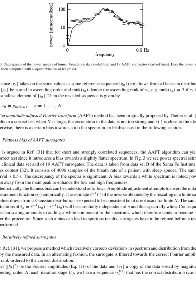
Fig. 3. Discrepancy of the power spectra of human breath rate data (solid line) and 19 AAFT surrogates (dashed lines). Here the power spectra have been computed with a square window of length 64.
sequence{rn}takes on the same values as some reference sequence{gn}(e.g. draws from a Gaussian distribution). Let{gn}be sorted in ascending order and rank(sn)denote the ascending rank ofsn, e.g. rank(sn)=3 ifsnis the 3rd smallest element of{sn}. Then the rescaled sequence is given by
rn=grank(sn), n=1, . . . , N. (10)
The amplitude adjusted Fourier transform (AAFT) method has been originally proposed by Theiler et al. [6]. It results in a correct test whenNis large, the correlation in the data is not too strong ands(·)is close to the identity. Otherwise, there is a certain bias towards a too flat spectrum, to be discussed in the following section.
4.2. Flatness bias of AAFT surrogates
It is argued in Ref. [31] that for short and strongly correlated sequences, the AAFT algorithm can yield an incorrect test since it introduces a bias towards a slightly flatter spectrum. In Fig. 3 we see power spectral estimates of a clinical data set and of 19 AAFT surrogates. The data is taken from data set B of the Santa Fe Institute time series contest [32]. It consists of 4096 samples of the breath rate of a patient with sleep apnoea. The sampling interval is 0.5 s. The discrepancy of the spectra is significant. A bias towards a white spectrum is noted: power is taken away from the main peak to enhance the low and high frequencies.
Heuristically, the flatness bias can be understood as follows. Amplitude adjustment attempts to invert the unknown measurement functions(·)empirically. The estimatesˆ−1(·)of the inverse obtained by the rescaling of a finite sample to values drawn from a Gaussian distribution is expected to be consistent but it is not exact for finiteN. The sampling fluctuations ofδn= ˆs−1(sn)−s−1(sn)will be essentially independent ofnand thus spectrally white. Consequently, Gaussian scaling amounts to adding a white component to the spectrum, which therefore tends to become flatter under the procedure. Since such a bias can lead to spurious results, surrogates have to be refined before a test can be performed.
4.3. Iteratively refined surrogates
In Ref. [31], we propose a method which iteratively corrects deviations in spectrum and distribution from the goal set by the measured data. In an alternating fashion, the surrogate is filtered towards the correct Fourier amplitudes and rank-ordered to the correct distribution.
Let{|Sk|2}be the Fourier amplitudes (Eq. (7)) of the data and{ck}a copy of the data sorted by magnitude in ascending order. At each iteration stage(i), we have a sequence{¯rn(i)}that has the correct distribution (coincides
with{ck}when sorted), and a sequence{¯sn(i)}that has the correct Fourier amplitudes given by{|Sk|2}. One can start with{¯rn(0)}being either an AAFT surrogate, or simply a random shuffle of the data.
The stepr¯n(i) → ¯s(i)n is a very crude “filter” in the Fourier domain: The Fourier amplitudes are simply replaced by the desired ones. First, take the (discrete) Fourier transform of{¯rn(i)}:
¯ Rk(i)=√1 N NX−1 n=0 ¯ rnexp i2πkn N . (11)
Then transform back, replacing the actual amplitudes by the desired ones, but keeping the phases exp(iψk(i))=
¯ Rk(i)/| ¯Rk(i)|: ¯ sn(i)= √1 N NX−1 k=0
exp(iψk(i))|Sk|exp
−i2πNkn
. (12)
The steps¯(i)n → ¯rn(i+1)proceeds by rank ordering:
¯
r(i+1)
n =crank(s¯(i)n ). (13)
It can be heuristically understood that the iteration scheme is attracted to a fixed pointr¯n(i+1)= ¯rn(i)for large(i). Since the minimal possible change is equal to the smallest nonzero differencecn−cn−1and is therefore finite for
finiteN, the fixed point is reached after a finite number of iterations. The remaining discrepancy betweenr¯n(∞)and
¯
sn(∞)can be taken as a measure of the accuracy of the method. Whether the residual bias inr¯n(∞)ors¯(n∞) is more tolerable depends on the data and the nonlinearity measure to be used. For coarsely digitised data,3 deviations from the discrete distribution can lead to spurious results whencer¯n(∞)is the safer choice. If linear correlations are dominant,s¯n(∞)can be more suitable.
The final accuracy that can be reached depends on the size and structure of the data and is generally sufficient for hypothesis testing. In all the cases we have studied so far, we have observed a substantial improvement over the standard AAFT approach. Convergence properties are also discussed in [31]. In Section 5.5 below, we will say more about the remaining inaccuracies.
4.4. Example: Southern Oscillation Index
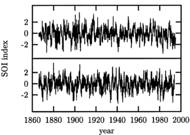
As an illustration let us perform a statistical test for nonlinearity on a monthly time series of the Southern Oscillation Index (SOI) from 1866 to 1994 (1560 samples). For a reference on analysis of Southern Oscillation data see Graham et al. [33]. Since a discussion of this climatic phenomenon is not relevant to the issue at hand, let us just consider the time series as an isolated data item. Our null hypothesis is that the data are adequately described by its single time probability distribution and its power spectrum. This corresponds to the assumption that an autoregressive moving average (ARMA) process is generating a sequence that is measured through a static monotonic, possibly nonlinear observation function.
For a test at the 99% level of significance (α=0.01), we generate a collection of 1/α−1=99 surrogate time series which share the single time sample probability distribution and the periodogram estimator with the data. This is carried out using the iterative method described in Section 4.3 above (see also Ref. [31]). Fig. 4 shows the data together with one of the 99 surrogates.
3Formally, digitisation is a non-invertible, nonlinear measurement and thus not included in the null hypothesis. Constraining the surrogates
to take exactly the same (discrete) values as the data seems to be reasonably safe, though. Since for that case we have not seen any dubious rejections due to discretisation, we did not discuss this issue as a serious caveat. This decision may of course prove premature.
Fig. 4. Monthly values of the Southern Oscillation Index (SOI) from 1866 to 1994 (upper trace) and a surrogate time series exhibiting the same auto-covariance function (lower trace). All linear properties of the fluctuations and oscillations are the same between both tracings. However, any possible nonlinear structure except for a static rescaling of the data is destroyed in the lower tracing by the randomisation procedure.
As a discriminating statistics we use a locally constant predictor in embedding space, using three dimensional delay coordinates at a delay time of one month. Neighbourhoods were selected at 0.2 times the RMS amplitude of the data. The test is set up in such a way that the null hypothesis may be rejected when the prediction error is smaller for the data than for all of the 99 surrogates. But, as we can see in Fig. 5, this is not the case. Predictability is not significantly reduced by destroying possible nonlinear structure. This negative result can mean several things. The prediction error statistics may just not have any power to detect the kind of nonlinearity present. Alternatively, the underlying process may be linear and the null hypothesis true. It could also be, and this seems the most likely option after all we know about the equations governing climate phenomena, that the process is nonlinear but the single time series at this sampling covers such a poor fraction of the rich dynamics that it must appear linear stochastic to the analysis.
Of course, our test has been carried out disregarding any knowledge of the SOI situation. It is very likely that more informed measures of nonlinearity may be more successful in detecting structure. We would like to point out, however, that if such information is derived from the same data, or literature published on it, a bias is likely to occur. Similarly to the situation of multiple tests on the same sample, the level of significance has to be adjusted properly. Otherwise, if many people try, someone will eventually, and maybe accidentally, find a measure that indicates nonlinear structure.
Fig. 5. Nonlinear prediction error measured for the SOI data set (see Fig. 4) and 99 surrogates. The value for the original data is plotted with a longer impulse. The mean and standard deviation of the statistic obtained from the surrogates is also represented by an error bar. It is evident that the data are not singled out by this property and we are unable to reject the null hypothesis of a linear stochastic stationary process, possibly rescaled by a nonlinear measurement function.
4.5. Periodicity artefacts
The randomisation schemes discussed so far all base the quantification of linear correlations on the Fourier amplitudes of the data. Unfortunately, that is not exactly what we want. Remember that the autocorrelation structure given by C(τ)=N1−τ N X n=τ+1 snsn−τ (14)
corresponds to the Fourier amplitudes only if the time series is one period of a sequence that repeats itself everyN time steps. This is, however, not what we believe to be the case. Neither is it compatible with the null hypothesis. Conserving the Fourier amplitudes of the data means that the periodic auto-covariance function
Cp(τ)=N1 N
X
n=1
snsmod(n−τ−1,N)+1 (15)
is reproduced, rather thanC(τ). This seemingly harmless difference can lead to serious artefacts in the surrogates, and, consequently, spurious rejections in a test. In particular, any mismatch between the beginning and the end of a time series poses problems, as discussed e.g. in Ref. [7]. In spectral estimation, problems caused by edge effects are dealt with by windowing and zero padding. None of these techniques have been successfully implemented for the phase randomisation of surrogates since they destroy the invertibility of the transform.
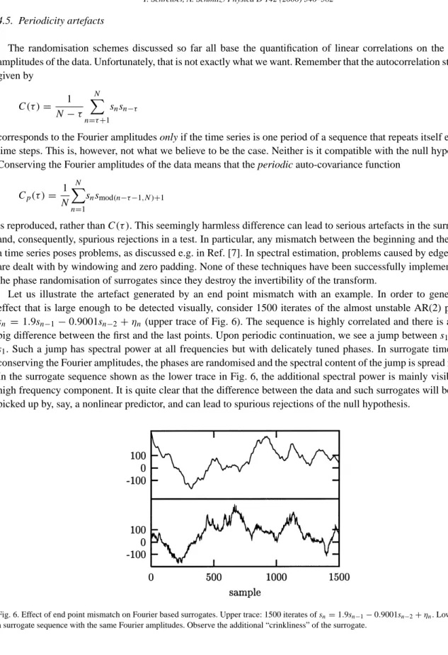
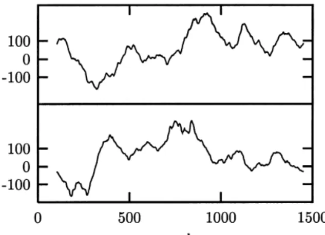
Let us illustrate the artefact generated by an end point mismatch with an example. In order to generate an effect that is large enough to be detected visually, consider 1500 iterates of the almost unstable AR(2) process,
sn =1.9sn−1−0.9001sn−2+ηn (upper trace of Fig. 6). The sequence is highly correlated and there is a rather
big difference between the first and the last points. Upon periodic continuation, we see a jump betweens1500and
s1. Such a jump has spectral power at all frequencies but with delicately tuned phases. In surrogate time series conserving the Fourier amplitudes, the phases are randomised and the spectral content of the jump is spread in time. In the surrogate sequence shown as the lower trace in Fig. 6, the additional spectral power is mainly visible as a high frequency component. It is quite clear that the difference between the data and such surrogates will be easily picked up by, say, a nonlinear predictor, and can lead to spurious rejections of the null hypothesis.
Fig. 6. Effect of end point mismatch on Fourier based surrogates. Upper trace: 1500 iterates ofsn=1.9sn−1−0.9001sn−2+ηn. Lower trace: a surrogate sequence with the same Fourier amplitudes. Observe the additional “crinkliness” of the surrogate.
Fig. 7. Repair of end point mismatch by selecting a sub-sequence of length 1350 of the signal shown in Fig. 6 that has an almost perfect match of end points. The surrogate shows no spurious high frequency structure.
The problem of non-matching ends can often be overcome by choosing a sub-interval of the recording such that the end points do match as closely as possible [34]. The possibly remaining finite phase slip at the matching points usually is of lesser importance. It can become dominant, though, if the signal is otherwise rather smooth. As a systematic strategy, let us propose to measure the end point mismatch by
γjump =PN(s1−sN)2
n=1(sn− hsi)2
(16) and the mismatch in the first derivative by
γslip =[(s2−Ps1)N −(sN−sN−1)]2
n=1(sn− hsi)2
. (17)
The fractionsγjumpandγslipgive the contributions to the total power of the series of the mismatch of the end points and the first derivatives, respectively. For the series shown in Fig. 6,γjump =0.45% and the end effect dominates the high frequency end of the spectrum. By systematically going through shorter and shorter sub-sequences of the data, we find that a segment of 1350 points starting at sample 102 yieldsγjump =0.00001% or an almost perfect match. That sequence is shown as the upper trace of Fig. 7, together with a surrogate (lower trace). The spurious “crinkliness” is removed.
In practical situations, the matching of end points is a simple and mostly sufficient precaution that should not be neglected. Let us mention that the SOI data discussed before is rather well behaved with little end-to-end mismatch (γjump <0.004%). Therefore there was no need to worry about the periodicity artefact.
The only method that has been proposed so far that strictly implements the standard autocorrelation, Eq. (14), rather than the periodic autocorrelation, Eq. (15), is given in Ref. [26] and will be discussed in detail in Section 5 below. The method is very accurate but also rather costly in terms of computer time. It should be used in cases of doubt and whenever a suitable sub-sequence cannot be found.
4.6. Iterative multivariate surrogates
A natural generalisation of the null hypothesis of a Gaussian linear stochastic process is that of a multivariate process of the same kind. In this case, the process is determined by giving the cross-spectrum in addition to the
power spectrum of each of the channels. In Ref. [35], it has been pointed out that phase randomised surrogates are readily produced by multiplying the Fourier phases of each of the channels by the same set of random phases since the cross-spectrum reflects relative phases only. The authors of Ref. [35] did not discuss the possibility to combine multivariate phase randomisation with an amplitude adjustment step. The extension of the iterative refinement scheme introduced in Section 4.3 to the multivariate case is relatively straightforward. Since deviations from a Gaussian distribution are very common and may occur due to a simple invertible rescaling due to the measurement process, we want to give the algorithm here.
Recall that the iterative scheme consists of two procedures which are applied in an alternating fashion until convergence to a fixed point is achieved. The amplitude adjustment procedure by rank ordering (13) is readily applied to each channel individually. However, the spectral adjustment in the Fourier domain has to be modified. Let us introduce a second index in order to denote theMdifferent channels of a multivariate time series{sn,m, n= 1, . . . , N, m = 1, . . . , M}. The change that has to be applied to the “filter” step, Eq. (12), is that the phases
ψk,mhave to be replaced by phasesφk,m with the following properties. (We have dropped the superscript(i)for convenience.) The replacement should be minimal in the least-squares sense, i.e. it should minimise
hk = M
X
m=1
|exp[iφk,m]−exp[iψk,m]|2. (18)
Also, the new phases must implement the same phase differences exhibited by the corresponding phases exp[iρk,m]=
Sk,m/|Sk,m|of the data:
exp[i(φk,m2−φk,m1)]=exp[i(ρk,m2 −ρk,m1)]. (19) The last equation can be fulfilled by settingφk,m=ρk,m+αk. With this, we havehk =PMm=12−2 cos(αk−
ψk,m+ρk,m)that is extremal when tanαk = PM m=1sin(ψk,m−ρk,m) PM m=1cos(ψk,m−ρk,m) . (20)
The minimum is selected by takingαkin the correct quadrant.
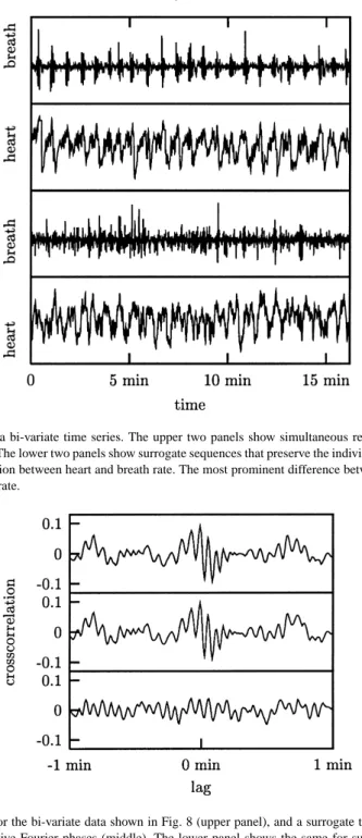
As an example, let us generate a surrogate sequence for a simultaneous recording of the breath rate and the instantaneous heart rate of a human during sleep. The data are again taken from data set B of the Santa Fe Institute time series contest [32]. The 1944 data points are an end-point matched sub-sequence of the data used as a multivariate example in Ref. [26]. In the latter study, which will be commented on in Section 6.2 below, the breath rate signal had been considered to be an input and therefore not randomised. Here, we will randomise both channels under the condition that their individual spectra as well as their cross-correlation function are preserved as good as possible while matching the individual distributions exactly. The iterative scheme introduced above took 188 iterations to converge to a fixed point. The data and a bi-variate surrogate are shown in Fig. 8. In Fig. 9, the cross-correlation functions of the data and one surrogate are plotted. Also, for comparison, the same for two individual surrogates of the two channels. The most striking difference between data and surrogates is that the coherence of the breath rate is lost. Thus, it is indeed reasonable to exclude the nonlinear structure in the breath dynamics from a further analysis of the heart rate by taking the breath rate as a given input signal. Such an analysis is however beyond the scope of the method discussed in this section. First of all, specifying the full cross-correlation function to a fixed signal plus the autocorrelation function over-specifies the problem and there is no room for randomisation. In Section 6.2 below, we will therefore revisit this problem. With the general constrained randomisation scheme to be introduced below, it will be possible to specify a limited number of lags of the auto- and cross-correlation functions.
Fig. 8. Simultaneous surrogates for a bi-variate time series. The upper two panels show simultaneous recordings of the breath rate and the instantaneous heart rate of a human. The lower two panels show surrogate sequences that preserve the individual distributions and power spectra as well as the cross-correlation function between heart and breath rate. The most prominent difference between data and surrogates is the lack of coherence in the surrogate breath rate.
Fig. 9. Cross-correlation functions for the bi-variate data shown in Fig. 8 (upper panel), and a surrogate that preserves the individual spectra and distributions as well as the relative Fourier phases (middle). The lower panel shows the same for surrogates prepared for each channel individually, i.e. without explicitly preserving the cross-correlation structure.
5. General constrained randomisation
Randomisation schemes based on the Fourier amplitudes of the data are appropriate in many cases. However, there remain some flaws, the strongest being the severely restricted class of testable null hypotheses. The periodogram
estimator of the power spectrum is about the only interesting observable that allows for the solution of the inverse problem of generating random sequences under the condition of its given value.
In the general approach of Ref. [26], constraints (e.g. autocorrelations) on the surrogate data are implemented by a cost function which has a global minimum when the constraints are fulfilled. This general framework is much more flexible than the Fourier based methods. We will therefore discuss it in some detail.
5.1. Null hypotheses, constraints, and cost functions
As we have discussed previously, we will often have to specify a null hypothesis in terms of a complete set of observable properties of the data. Only in specific cases (e.g. the two point autocorrelation function), there is a one-to-one correspondence to a known class of models (here the ARMA process). In any case, if{¯sn}denotes a surrogate time series, the constraints will most often be of (or can be brought into) the form
Fi({¯sn})=0, i=1, . . . , I. (21) Such constraints can always be turned into a cost function
E({¯sn})= I X i=1 |wiFi({¯sn})|q !1/q . (22)
The fact thatE({¯sn})has a global minimum when the constraints are fulfilled is unaffected by the choice of the weightswi 6=0 and the orderqof the average. The least-squares orL2average is obtained atq =2,L1atq =1 and the maximum distance whenq → ∞. Geometric averaging is also possible (and can be formally obtained by taking the limitq →0 in a proper way). We have experimented with different choices ofqbut we have not found a choice that is uniformly superior to others. It seems plausible to give either uniform weights or to enhance those constraints which are particularly difficult to fulfill. Again, conclusive empirical results are still lacking.
Consider as an example the constraint that the sample autocorrelation function of the surrogateC(τ)¯ = h¯sns¯n−τi (data rescaled to zero mean and unit variance) are the same as those of the data,C(τ)= hsnsn−τi. This is done by specifying zero discrepancy as a constraintFτ({¯sn})= ¯C(τ)−C(τ), τ =1, . . . , τmax. If the correlations decay fast,τmaxcan be restricted, otherwiseτmax=N−1 (the largest available lag). Thus, a possible cost function could read
E=maxτmaxτ=0| ¯C(τ)−C(τ)|. (23) Other choices ofqand the weights are of course also possible.
In all the cases considered in this paper, one constraint will be that the surrogates take on the same values as the data but in different time order. This ensures that data and surrogates can equally likely be drawn from the same (unknown) single time probability distribution. This particular constraint is not included in the cost function but identically fulfilled by considering only permutations without replacement of the data for minimisation.
By introducing a cost function, we have turned a difficult nonlinear, high dimensional root finding problem (21) into a minimisation problem (22). This leads to extremely many false minima whence such a strategy is discouraged for general root finding problems [43]. Here, the situation is somewhat different since we need to solve Eq. (21) only over the set of all permutations of{sn}. Although this set is big, it is still discrete and powerful combinatorial minimisation algorithms are available that can deal with false minima very well. We choose to minimiseE({¯sn}) among all permutations{¯sn}of the original time series{sn}using the method of simulated annealing. Configurations are updated by exchanging pairs in{¯sn}. The annealing scheme will decide which changes to accept and which to reject. With an appropriate cooling scheme, the annealing procedure can reach any desired accuracy. Apart from
our particular minimisation problem. Since the detailed behaviour will be different for each cost function, we can only give some general guidelines.
The main idea behind simulated annealing is to interpret the cost functionEas an energy in a thermodynamic system. Minimising the cost function is then equivalent to finding the ground state of a system. A glassy solid can be brought close to the energetically optimal state by first heating it and subsequently cooling it. This procedure is called “annealing”, hence the name of the method. If we want to simulate the thermodynamics of this tempering procedure on a computer, we notice that in thermodynamic equilibrium at some finite temperatureT, system configurations should be visited with a probability according to the Boltzmann distribution e−E/T of the canonical ensemble. In Monte Carlo simulations, this is achieved by accepting changes of the configuration with a probabilityp=1 if the energy is decreased(1E <0)andp=e−1E/T if the energy is increased(1E ≥0). This selection rule is often referred to as the Metropolis step. In a minimisation problem, the temperature is the parameter in the Boltzmann distribution that sets its width. In particular, it determines the probability to go “up hill”, that is important if we need to get out of false minima.
In order to anneal the system to the ground state of minimal “energy”, i.e. the minimum of the cost function, we want to first “melt” the system at a high temperatureT, and then decreaseT slowly, allowing the system to be close to thermodynamic equilibrium at each stage. If the changes to the configuration we allow to be made connect all possible states of the system, the updating algorithm is called ergodic. Although some general rigorous convergence results are available, in practical applications of simulated annealing some problem-specific choices have to be made. In particular, apart from the constraints and the cost function, one has to specify a method of updating the configurations and a schedule for lowering the temperature. In the following, we will discuss each of these issues. Concerning the choice of cost function, we have already mentioned that there is a large degeneracy in that many cost functions have an absolute minimum whenever a given set of constraints is fulfilled. The convergence properties can depend dramatically on the choice of cost function. Unfortunately, this dependence seems to be so complicated that it is impossible even to discuss the main behaviour in some generality. In particular, the weightswi in Eq. (22) are sometimes difficult to choose. Heuristically, we would like to reflect changes in the I different constraints approximately equally, provided the constraints are independent. Since their scale is not at all set by Eq. (21), we can use thewi for this purpose. Whenever we have some information about which kind of deviation would be particularly problematic with a given test statistic, we can give it a stronger weight. Often, the shortest lags of the autocorrelation function are of crucial importance, whence we tend to weight autocorrelations by 1/τ when they occur in sums. Also, theC(τ)with largerτ are increasingly ill-determined due to the fewer data points entering the sums. As an extreme example,C(N−1)=s1sN−1shows huge fluctuations due to the lack of self-averaging.
Finally, there are many moreC(τ)with largerτ than at the crucial short lags.
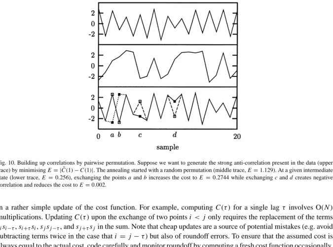
A way to efficiently reach all permutations by small individual changes is by exchanging randomly chosen (not necessarily close-by) pairs. How the interchange of two points can affect the current cost is illustrated schematically in Fig. 10. Optimising the code that computes and updates the cost function is essential since we need its current value at each annealing step — which are expected to be many. Very often, an exchange of two points is reflected
Fig. 10. Building up correlations by pairwise permutation. Suppose we want to generate the strong anti-correlation present in the data (upper trace) by minimisingE= | ¯C(1)−C(1)|. The annealing started with a random permutation (middle trace,E=1.129). At a given intermediate state (lower trace,E=0.256), exchanging the pointsaandbincreases the cost toE=0.2744 while exchangingcanddcreates negative correlation and reduces the cost toE=0.002.
in a rather simple update of the cost function. For example, computingC(τ)for a single lagτ involves O(N) multiplications. UpdatingC(τ)upon the exchange of two pointsi < j only requires the replacement of the terms
sisi−τ,si+τsi,sjsj−τ, andsj+τsjin the sum. Note that cheap updates are a source of potential mistakes (e.g. avoid subtracting terms twice in the case thati=j−τ) but also of roundoff errors. To ensure that the assumed cost is always equal to the actual cost, code carefully and monitor roundoff by computing a fresh cost function occasionally. Further speed-up can be achieved in two ways. Often, not all the terms in a cost function have to be added up until it is clear that the resulting change goes uphill by an amount that will lead to a rejection of the exchange. Also, pairs to be exchanged can be selected closer in magnitude at low temperatures because large changes are very likely to increase the cost.
Many cooling schemes have been discussed in the literature [39]. We use an exponential scheme in our work. We will give details on the — admittedly largely ad hoc — choices that have been made in the TISEAN implementation in Appendix A. We found it convenient to have a scheme available that automatically adjusts parameters until a given accuracy is reached. This can be done by cooling at a certain rate until we are stuck (no more accepted changes). If the cost is not low enough yet, we melt the system again and cool at a slower rate.
5.3. Example: avoiding periodicity artefacts
Let us illustrate the use of the annealing method in the case of the standard null hypothesis of a rescaled linear process. We will show how the periodicity artefact discussed in Section 4.5 can be avoided by using a more suitable cost function. We prepare a surrogate for the data shown in Fig. 6 (almost unstable AR(2) process) without truncating its length. We minimise the cost function given by Eq. (23), involving all lags up toτmax=100. Also, we excluded the first and last points from permutations as a cheap way of imposing the long range correlation. In Fig. 11 we show progressive stages of the annealing procedure, starting from a random scramble. The temperatureT is decreased by 0.1% after either 106permutations have been tried or 104have been successful. The final surrogate neither has
Fig. 11. Progressive stages of the simulated annealing scheme. The data used in Fig. 6 are used to generate an annealed surrogate that minimises
E=max100τ=0| ¯C(τ)−C(τ)|over all permutations of the data. From top to bottom, the values forEare: 0 (original data), 1.01 (random scramble),
0.51, 0.12, 0.015, and 0.00013.
spuriously matching ends nor the additional high frequency components we saw in Fig. 6. The price we had to pay was that the generation of one single surrogate took 6 h of CPU time on a Pentium II PC at 350 MHz. If we had taken care of the long range correlation by leaving the end points loose but takingτmax =N −1, convergence would have been prohibitively slow. Note that for a proper test, we would need at least 19 surrogates. We should stress that this example with its very slow decay of correlations is particularly nasty — but still feasible. Obviously, sacrificing 10% of the points to get rid of the end point mismatch is preferable here to spending several days of CPU time on the annealing scheme. In other cases, however, we may not have such a choice.
5.4. Combinatorial minimisation and accuracy
In principle, simulated annealing is able to reach arbitrary accuracy at the expense of computer time. We should, however, remark on a few points. Unlike other minimisation problems, we are not really interested in the solutions that putE=0 exactly. Most likely, these are the data set itself and a few simple transformations of it that preserve the cost function (e.g. a time reversed copy). On the other hand, combinatorics makes it very unlikely that we ever reach one of these few of theN! permutations, unlessN is really small or the constraints grossly over-specify the problem. This can be the case, e.g. if we include all possible lags of the autocorrelation function, which gives as
many (nonlinear) equations as unknowns,I =N. These may have the data itself as a unique solution for smallNin the space of permutations. In such extreme situations, it is possible to include extra cost terms penalising closeness to one of the trivial transformations of the data. Let us note that if the surrogates are “too similar” to the data, this does not in itself affect the validity of the test. Only the discrimination power is reduced.
Now, if we do not want to reachE=0, how can we be sure that there are enough independent realisations with
E≈0? The theoretical answer depends on the form of the constraints in a complicated way and cannot be given in general. We can, however, offer a heuristic argument that the number of configurations withEsmaller than some
1Egrows fast for largeN. Suppose that for largeN the probability distribution ofEconverges to an asymptotic formp(E). Assume further thatp(1E)˜ = Prob(E < 1E) = R01Ep(E)dEis nonzero but maybe very small. This is evidently true, e.g. for autocorrelations. Thus, while the probability to findE < 1Ein a random draw from the distribution of the data may be extremely small, sayp(1E)˜ =10−45at 10 sigmas from the mean energy, the total number of permutations, figuring as the number of draws, grows asN! ≈(N/e)N√2πN, i.e., much faster than exponentially. Thus, we expect the number of permutations withE < 1Eto be∝ ˜p(1E)N!. For example, 10−45×1000!≈102522.
In any case, we can always monitor the convergence of the cost function to avoid spurious results due to residual inaccuracy in the surrogates. As we will discuss below, it can also be a good idea to test the surrogates with a linear test statistic before performing the actual nonlinearity test.
5.5. The curse of accuracy
Strictly speaking, the concept of constrained realisations requires the constraints to be fulfilled exactly, a practical impossibility. Most of the research efforts reported in this article have their origin in the attempt to increase the accuracy with which the constraints are implemented, i.e. to minimise the bias resulting from any remaining discrepancy. Since most measures of nonlinearity are also sensitive to linear correlations, a side effect of the reduced bias is a reduced variance of such estimators. Paradoxically, the enhanced accuracy may result in false rejections of the null hypothesis on the ground of tiny differences in some nonlinear characteristics. This important point has been recently put forth by Kugiumtzis [40].
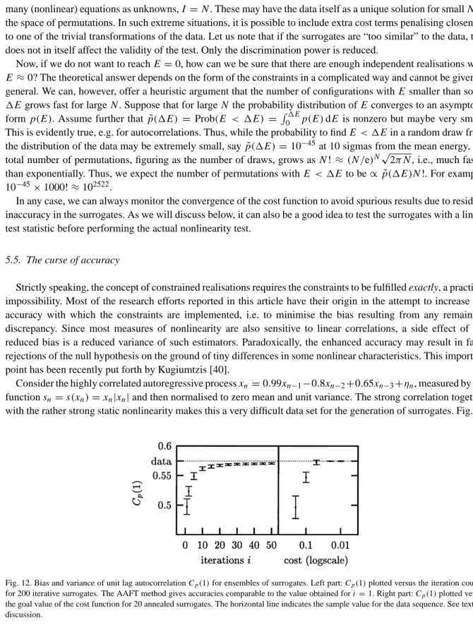
Consider the highly correlated autoregressive processxn=0.99xn−1−0.8xn−2+0.65xn−3+ηn, measured by the
functionsn =s(xn)=xn|xn|and then normalised to zero mean and unit variance. The strong correlation together with the rather strong static nonlinearity makes this a very difficult data set for the generation of surrogates. Fig. 12
Fig. 12. Bias and variance of unit lag autocorrelationCp(1)for ensembles of surrogates. Left part:Cp(1)plotted versus the iteration counti for 200 iterative surrogates. The AAFT method gives accuracies comparable to the value obtained fori=1. Right part:Cp(1)plotted versus the goal value of the cost function for 20 annealed surrogates. The horizontal line indicates the sample value for the data sequence. See text for discussion.
Kugiumtzis [40] suggests to test the validity of the surrogate sample by performing a test using a linear statistic for normalisation. For the data shown in Fig. 12, this would have detected the lack of convergence of the iterative surrogates. Currently, this seems to be the only way around the problem and we thus recommend to follow his suggestion. With the much more accurate annealed surrogates, we have not so far seen examples of dangerous remaining inaccuracy, but we cannot exclude their possibility. If such a case occurs, it may be possible to generate unbiased ensembles of surrogates by specifying a cost function that explicitly minimises the bias. This would involve the whole collection ofMsurrogates at the same time, including extra terms like
Eensemble= τmax X τ=0 M X m=1 ¯ Cm(τ)−C(τ) !2 . (24)
Here,C¯m(τ)denotes the autocorrelation function of themth surrogate. In any event, this will be a very cumbersome procedure, in terms of implementation and in terms of execution speed and it is questionable if it is worth the effort.
6. Various examples
In this section, we want to give a number of applications of the constrained randomisation approach. If the constraints consist only of the Fourier amplitudes and the single time probability distribution, the iteratively refined, amplitude adjusted surrogates [31] discussed in Section 4.3 are usually sufficient if the end point artefact can be controlled and convergence is satisfactory. Even the slightest extension of these constraints makes it impossible to solve the inverse problem directly and we have to follow the more general combinatorial approach discussed in the previous section. The following examples are meant to illustrate how this can be carried out in practice.
6.1. Including non-stationarity
Constrained randomisation using combinatorial minimisation is a very flexible method since, in principle, arbitrary constraints can be realised. Although it is seldom possible to specify a formal null hypothesis for more general constraints, it can be quite useful to be able to incorporate into the surrogates any feature of the data that is understood already or that is uninteresting. Non-stationarity has been excluded so far by requiring the equations defining the null hypothesis to remain constant in time. This has a two-fold consequence. First, and most importantly, we must keep in mind that the test will have discrimination power against non-stationary signals as a valid alternative to the null hypothesis. Thus a rejection can be due to nonlinearity or non-stationarity equally well.
Second, if we do want to include non-stationarity in the null hypothesis we have to do so explicitly. Let us illustrate how this can be done with an example from finance. The time series consists of 1500 daily returns (until the end of 1996) of the BUND Future, a derived German financial instrument. The data were kindly provided by Thomas
Fig. 13. Non-stationary financial time series (BUND Future returns, top) and a surrogate (bottom) preserving the non-stationary structure quantified by running window estimates of the local mean and variance (middle).
Schürmann, WGZ-Bank Düsseldorf. As can be seen in the upper panel of Fig. 13, the sequence is non-stationary in the sense that the local variance and to a lesser extent also the local mean undergo changes on a time scale that is long compared to the fluctuations of the series itself. This property is known in the statistical literature as
heteroscedasticity and modelled by the so-called GARCH [41] and related models. Here, we want to avoid the
construction of an explicit model from the data but rather ask the question if the data is compatible with the null hypothesis of a correlated linear stochastic process with time dependent local mean and variance. We can answer this question in a statistical sense by creating surrogate time series that show the same linear correlations and the same time dependence of the running mean and running variance as the data and comparing a nonlinear statistic between data and surrogates. The lower panel in Fig. 13 shows a surrogate time series generated using the annealing method. The cost function was set up to match the autocorrelation function up to five days and the moving mean and variance in sliding windows of 100 days duration. In Fig. 13 the running mean and variance are shown as points and error bars, respectively, in the middle trace. The deviation of these between data and surrogate has been minimised to such a degree that it can no longer be resolved. A comparison of the time-asymmetry statistic Eq. (3) for the data and 19 surrogates did not reveal any discrepancy, and the null hypothesis could not be rejected.
6.2. Multivariate data
In Ref. [26], the flexibility of the approach was illustrated by a simultaneous recording of the breath rate and the instantaneous heart rate of a human subject during sleep. The interesting question was, how much of the structure in the heart rate data can be explained by linear dependence on the breath rate. In order to answer this question, surrogates were made that had the same autocorrelation structure but also the same cross-correlation with respect to the fixed input signal, the breath rate. While the linear cross-correlation with the breath rate explained the coherent structure of the heart rate, other features, in particular its asymmetry under time reversal, remained unexplained. Possible explanations include artefacts due to the peculiar way of deriving heart rate from inter-beat intervals, nonlinear coupling to the breath activity, nonlinearity in the cardiac system, and others.
Within the general framework, multivariate data can be treated very much the same way as scalar time series. In the above example, we chose to use one of the channels as a reference signal which was not randomised. The